BCS Superconductivity in Quantum Critical Metals

Abstract

We present a simple phenomenological scaling theory for the pairing instability of a quantum critical metal. It can be viewed as a minimal generalization of the classical Bardeen-Cooper-Schrieffer theory of superconductivity for normal Fermi-liquid metals. We assume that attractive interactions are induced in the fermion system by an external ’bosonic glue’ that is strongly retarded. Resting on the small Migdal parameter, all the required information from the fermion system needed to address the superconductivity enters through the pairing susceptibility. Asserting that the normal state is a strongly interacting quantum critical state of fermions, the form of this susceptibility is governed by conformal invariance and one only has the scaling dimension of the pair operator as free parameter. Within this scaling framework, conventional BCS theory appears as the ’marginal’ case but it is now easily generalized to the (ir)relevant scaling regimes. In the relevant regime an algebraic singularity takes over from the BCS logarithm with the obvious effect that the pairing instability becomes stronger. However, it is more surprising that this effect is strongest for small couplings and small Migdal parameters, highlighting an unanticipated important role of retardation. Using exact forms for the finite temperature pair susceptibility from 1+1D conformal field theory as models, we study the transition temperatures, finding that the gap to transition temperature ratio’s are generically large compared to the BCS case, showing however an opposite trend as function of the coupling strength compared to conventional Migdal-Eliashberg theory. We show that our scaling theory naturally produces the superconducting ’domes’ surrounding the quantum critical points, even when the coupling to the glue itself is not changing at all. We argue that hidden relations will exist between the location of the cross-over lines to the Fermi-liquids away from the quantum critical points , and the detailed form of the dome when the glue strength is independent of the zero temperature control parameter. Finally, we discuss the behavior of the orbital limited upper critical magnetic field as function of the zero temperature coupling constant. Compared to the variation of the transition temperature, the critical field might show a much stronger variation pending the value of the dynamical critical exponent.

I Introduction

The ’mystery superconductors’ of current interest share the property that their normal states are poorly understood ’non Fermi-liquids’. Experiments reveal that these are governed by a scale invariance of their quantum dynamics. The best documented examples are found in the heavy fermion (HF) systemsMathur et al. (1998); Zaanen (2008); Stewart (2006); von Löhneisen et al. (2007); Coleman et al. (2001); Coleman and Schofield (2005); Gegenwart et al. (2008); Paschen et al. (2004); Si et al. (2001). As function of pressure or magnetic field one can drive a magnetic phase transition to zero temperature. On both sides of this quantum critical point (QCP) one finds Fermi-liquids characterized by quasiparticle masses that tend to diverge at the QCP. At the QCP one finds a ’strange metal’ revealing traits of scale invariance, while at a ’low’ temperature a transition follows most often to a superconducting state with a maximum $T_{c}$ right at the QCP. It is widely believed that a similar ’fermionic quantum criticality’ is governing the normal state in optimally doped cuprate high Tc superconductors. The best evidence is perhaps the ’Planckian’ relaxation time observed in transport experiments $\tau_{\hbar}\simeq\hbar/(k_{B}T)$van der Marel et al. (2003); Cooper et al. (2009) indicating that this normal state has no knowledge of the scale $E_{F}$ since in a Fermi-liquid $\tau=(E_{F}/k_{B}T)\tau_{\hbar}$. Very recently indications have been found that even the iron based superconductors might be governed by quantum critical normal states associated with a magnetic and/or structural zero temperature transition, giving rise to a novel scaling behavior of the electronic specific heatBud’ko et al. (2009); Zaanen (2009).

The idea that superconductivity can be caused by a quantum phase transition involving a bosonic order parameter has a long history, starting with the marginal Fermi-liquid ideas of VarmaVarma et al. (1989) in the context of cuprates of the late 1980’s and the ideas of spin-fluctuation driven heavy fermion superconductivity dating back to Lonzarich et al.Mathur et al. (1998). The bulk of the large theoretical literatureMonthoux et al. (2007); Chubukov and Sachdev (1993); Varma et al. (2002); Bonesteel et al. (1996); Galitski and Sachdev (2009); Chubukov and Schmalian (2005); Chubukov and Tsvelik (2007); Abanov et al. (2001a, b); Chubukov et al. (2003); Krotkov and Chubukov (2006a); Krotkov and Chubukov (2006b); Abanov et al. (2008); Khveshchenko and Shively (2006); Moon and Sachdev (2009); Fisk and Pines (1998); Mazin and Singh (1997); Monthoux and Lonzarich (1999); Fay and Appel (1980); Millis et al. (1988); Franz and Millis (1998); Roussev and Millis (2001); Blagoev et al. (1999); Wang et al. (2001); Allen and Dynes (1975); Marsiglio and Carbotte (1986); Carbotte (1990); Scalapino et al. (1986); Bulaevskii and Zyskin (1990); Kirkpatrick et al. (2001); Sandeman et al. (2003); Strack et al. (2009); Son (1999); Dolgov and Maksimov (1982); Dolgov et al. (2008); Combescot (1997) dealing with this subject that evolved since then departs from an assumption dating back to the seminal work of Herz in the 1970’sHertz (1976). This involves the nature of the ultraviolet: at some relatively short time scale where the electron system has closely approached a Fermi-liquid the influence of the critical order parameter fluctuations become noticable. The Fermi surface and Fermi energy of this quasiparticle system can then be used as building blocks together with the bosonic field theory describing the critical order parameter fluctuations to construct a perturbative framework dealing with the coupling between these fermionic- and bosonic sectors. The lowest order effect of this coupling is that the fermi gas of quasiparticles acts as a heat bath damping the bosonic order parameter fluctuations, with the effect that the effective space-time dimensionality of the bosonic field theory exceeds the upper critical dimension. These dressed order parameter fluctuations than ’back react’ on the quasiparticle system causing ’singular’ interactions in the Cooper channel, yielding in turn a rational for a generic ’high Tc’ superconductivity at QCP’s.

The crucial assumption in this ’Herz philosophy’ is that the fermion physics is eventually controlled by the Fermi gas. In the cases of empirical interest it is generally agreed that in the UV the interaction energies are much larger than the bare kinetic energies, while there is no obvious signature in the experiments for a renormalization flow that brings the system close to a weakly interacting fermion gas before entering the singular ’Herz’ critical regime. From the theoretical side, the introduction of this UV Fermi gas can be viewed as an intuitive leap. The only truly fermionic state of matter that is understood mathematically is the Fermi gas and its perturbative ’derivative’ (the Fermi liquid): the fermion sign problem makes it impossible to address fermionic matter in general mathematical termsTroyer and Wiese (2005). However, very recently the ’grib of the Fermi-gas’ has started to loosen specifically in the context of fermionic critical matter. A first step in this direction is the demonstration of proof of principle that truly critical fermionic states of matter can exist that have no knowledge whatever of the statistical Fermi energy scale: the fermionic Feynman backflow wavefunction AnsatzKrüger and Zaanen (2008). The substantive development is the recent work addressing fermion physics using the string theoretical AdS/CFT correspondence. It appears that this duality between quantum field theory and gravitational physics is capable of describing Fermi-liquids that emerge from a manifestly strongly interacting, critical ultravioletCubrovic et al. (2009). In another implementation, one finds an IR physics describing ’near’ Fermi-liquids characterized by ’critical’ Fermi surfacesSenthil (2008) controlled by an emergent conformal symmetry implying the absence of energy scales like the Fermi-energyLiu et al. (2009); Faulkner et al. (2009).

This lengthy consideration is required to motivate the subject of this paper: a phenomenological scaling theory for a Bardeen-Cooper-Schrieffer (BCS) type superconductivity starting from the postulate that the normal state is not a Fermi-liquid, but instead a truly conformal fermionic state of matter. With ’BCS type’ we mean the following: we assume as in BCS that besides the electron system a bosonic modes are present that cause attractive electron-electron interactions. This ’glue’ is retarded in the sense that the characteristic energy scale of this external bosonic system $\omega_{B}$ is small as compared to the ultraviolet cut-off scale of the quantum critical fermion system $\omega_{c}$ . Having a small Migdal parameter, the glue-electron vertex corrections can then be ignored and the the effects of the glue are described in terms of the Migdal-Eliashberg time dependent mean field theory, reducing to the static BCS mean field theory in the weak coupling limitSchrieffer (1971). All information coming from the electron system that is required for the pairing instability is encapsulated in the electronic pair susceptibility. Instead of using the Fermi gas pair susceptibility (as in conventional BCS), we rely on the fact that conformal invariance fixes the analytical form of this response function in terms of two free parameters: an overall UV cut-off scale ($T_{0}$) and the anomalous scaling dimension of the pair susceptibility, expressed in a dynamical critical exponent $z$ and correlation function exponent $\eta_{p}$. The outcome is a scaling theory for superconductivity that is in essence very simple; much of the technical considerations that follow are dealing with details associated with modeling accurately the effects of the breaking of conformal invariance by temperature and the superconducting instability. This theory is however surprisingly economical in yielding phenomenological insights. Conventional BCS appears as a special ’marginal’ case, and our main result is the generalized gap equation, Eq. (10). The surprise it reveals is the role of retardation: when the Migdal parameter $\omega_{B}/\omega_{c}$ is small (where the mathematical control is best) we find at small coupling constants $\tilde{\lambda}$ a completely different behavior compared to conventional BCS: the gap magnitude $\Delta$ becomes similar to the glue energy $\omega_{B}$. To illustrate the case with numbers, a moderate coupling to phonons like $\tilde{\lambda}=0.3$ with a frequency $\omega_{B}=50$ meV will yield rather independently of scaling dimensions a gap of 40 $meV$ and a $T_{c}$ of 100 Kelvin or so: these are numbers of relevance to cuprate superconductors!

The theory has more in store. Incorporating the motive that on both sides of the quantum critical point heavy Fermi liquids emerge from the quantum critical metal as in the heavy fermion systems, we show that the superconducting ’dome’ surrounding the quantum critical point emerges naturally without changing the coupling to the bosonic glue. The form of this dome is governed by the correlation length, but we find via the pair susceptibility a direct relation with the effective mass of the quasiparticles of the Fermi-liquids. Last but not least, we analyze the orbital limiting upper critical magnetic field, finding out that pending the value of the dynamical critical exponent it can diverge very rapidly upon approaching the QCP, offering an explanation for the observations in the ferromagnetic URhGe heavy fermion superconductorLevy et al. (2007).

The scaling phenomenology we present here is simple and obvious, but it appears to be overlooked so far. Earlier work by BalatskyBalatsky (1993), SudboSudbo (1995) and Yin and ChakravartyYin and Chakravarty (1996) is similar in spirit but yet quite different. These authors depart from a Luttinger liquid type single particle propagators to compute the pair susceptibility from the bare fermion particle-particle loop. Although this leads to pair susceptibility similar (although not identical) to ours, it is conceptually misleading since in any non Fermi-liquid, there is no such simple relation between two-point and four-point correlators. This is particularly well understood for conformal field theories: for the higher dimensional cases the AdS/CFT correspondence demonstrates that two point CFT correlators are determined by kinematics in AdS while the four- and higher point correlators require a tree level computationMuck and Viswanathan (1998); Freedman et al. (1999); D’Hoker and Freedman (1998a); Liu (1998); D’Hoker and Freedman (1998b); D’Hoker et al. (1999); Chalmers and Schalm (1998, 1999). More serious for the phenomenology, this older work ignores the role played by retardation; it is a-priori unclear whether one can construct a mathematically controlled scaling theory for BCS without the help of a small Migdal parameter.

The remainder of this paper is organized as follows. In section II we review a somewhat unfamiliar formulation of the classic BCS theory that makes very explicit the role of the pair susceptibility. We then introduce the scaling forms for the pair susceptibilities as follow from conformal invariance. By crudely treating the modifications in the pair susceptibility at low energies associated with the presence of the pair condensate we obtain the new gap equation Eq. (10). This catches already the essence of the BCS superconductivity of quantum critical metals and we discuss its implications in detail. In section III we focus in on intricacies associated with determining the transition temperature. Conformal invariance is now broken and one needs to know the scaling functions in some detail. We use the exact results of 1+1 dimensional conformal field theory as a model to address these matters. In section IV we turn to the harder problem of modeling the crossover from the large energy critical pair susceptibility to the low energy, zero temperature infrared that is governed by conventional Bogoliubov fermions, as needed to devise a more accurate zero temperature gap equation. The casual reader might want to skip both sections. The moral is that information on the cross-over behavior of the pair susceptibility is required that is beyond simple scaling considerations to address what happens when the conformal invariance is broken either by temperature (as of relevance to the value of $T_{c}$) or by the presence of the BCS condensate (of relevance for the zero temperature gap). The conclusion will be that although the gross behaviors are not affected, it appears to be impossible to compute numbers like the gap to $T_{c}$ ratio accurately since these are sensitive to the details of the cross-over behaviors. In section V we explore the theory away from the critical point, assuming that cross-overs follow to heavy Fermi-liquids, where we address the origin of the superconducting dome. Finally, in section VI we address the scaling behavior of the orbital limited upper critical field.

II BCS theory and the scaling of the pair susceptibility.

Let us first revisit the backbone of Migdal-Eliashberg theory. We need a formulation that is avoiding the explicit references to the Fermi gas of the text book formulation, but it is of course well known how to accomplish this. Under the condition of strong retardation and small couplings, the effects of the glue are completely enumerated by the gap equationAllen (1980) ignoring angular momentum channels ($s$,$d$ waves, etcetera) for the time being,

$$1-g\chi^{\prime}_{\rm ret}({\vec{q}}=0,\omega=0,\Delta,T)=0,$$ (1)

where $g$ is the effective coupling strength of the glue, while $\chi^{\prime}_{\rm ret}$ is the zero frequency value of the real part of the retarded pair susceptibility at a temperature $T$ in the presence of the gap $\Delta$. This effective $\chi^{\prime}_{\rm ret}$ also incorporates the effects of retardation. The textbooks with their focus on non-interacting electrons accomplish this in a rather indirect way, by putting constraints on momentum integrations. Retardation is however about time scales and the general way to incorporate retardation is by computing $\chi^{\prime}_{\rm ret}$ by employing the Kramers-Kronig relation starting from the imaginary part of the full electronic pair susceptibility $\chi_{p}^{\prime\prime}$. For a glue characterized by a single frequency $\omega_{B}$,

$$\chi^{\prime}_{\rm ret}(\omega=0)=2{\cal P}\int_{0}^{2\omega_{B}}d\omega^{\prime}\frac{\chi_{p}^{\prime\prime}(\omega^{\prime})}{\omega^{\prime}}.$$ (2)

with the full pair susceptibility given by the Kubo formula,

$$\chi_{p}({\vec{q}},\omega)=-i\int_{0}^{\infty}dte^{i(\omega+i\eta)t}\left\langle[b^{\dagger}({\vec{q}},0),b({\vec{q}},t)]\right\rangle,$$ (3)

associated with the pair operator $b^{\dagger}({\vec{q}},t)={\sum_{\vec{k}}}c^{\dagger}_{{\vec{k}}+\frac{\vec{q}}{2},\uparrow}(t)c^{\dagger}_{-{\vec{k}}+\frac{\vec{q}}{2},\downarrow}(t)$.

In the case of conventional superconductors the normal state is a Fermi-liquid, formed from (nearly) non-interacting quasiparticles. One can get away with a ’bare fermion loop’ pair susceptibility. The specialty of this pair susceptibility is that its imaginary part is frequency independent at zero temperature. It extends up to the Fermi energy of the Fermi-liquid and from the unitary condition,

$$\int_{0}^{\infty}\chi_{p}^{\prime\prime}(\omega)d\omega=1$$ (4)

it follows that at zero temperature $\chi^{\prime\prime}(\omega)=N_{0}=1/(2E_{F})$. In logarithmic accuracy the gap enters as the low frequency cut-off in Eq. (2) such that,

$$\chi^{\prime}_{\rm ret}(\omega=0,\Delta,T=0)=\int_{\Delta}^{2\omega_{B}}\frac{d\omega^{\prime}}{E_{F}\omega^{\prime}}=\frac{1}{E_{F}}\log\frac{2\omega_{B}}{\Delta},$$ (5)

and from Eq. (1) the famous BCS gap equation follows: $\Delta=2\omega_{B}e^{-1/\lambda}$, where $\lambda=g/E_{F}$.

This formulation of BCS has the benefit that it makes very explicit that all the information on the electron system required for the understanding of the pairing instability is encoded in the pair susceptibility. This is in turn a bosonic response function of the electron system since it involves the response of two fermions, much like the dynamical susceptibilities associated with charge- or spin densities. In addition one needs the fact that the pair density is a non-conserved quantity, in the same sense as a staggered magnetization. When the quantum system is conformal (i.e. the zero temperature quantum critical metal) the analytical form of the dynamical pair susceptibility is fixed at zero temperature by the requirement of invariance under scale transformationsSachdev (1999),

$$\chi(\omega)=\lim_{\delta\rightarrow 0}Z^{\prime\prime}(-(\omega+i\delta)^{2})^{-\frac{2-\eta_{p}}{2z}},$$ (6)

as determined by the a-priori unknown unknown exponents $\eta_{p}$ and $z$, the anomalous scaling dimension of the pair operator and the dynamical critical exponent, respectively. The normalization constant $Z^{\prime\prime}$ is via the unitarity condition Eq.(4) determined by the UV cut-off scale $\omega_{c}$. Because we invoke a small Migdal parameter we are interested in the ’deep infrared’ of the theory that is not very sensitive to the precise choice of this UV energy scale. A reasonable choice is the energy where the thermal de Broglie wavelength becomes of order of the electron separation, i.e. the Fermi energy of an equivalent system of non-interacting electrons. Defining $\alpha_{p}=\frac{2-\eta_{p}}{z}$ and using Eq. (4) with the cut-off scale $\omega_{c}$, we find,

$$Z^{\prime\prime}=\frac{1-\alpha_{p}}{\sin(\frac{\pi}{2}\alpha_{p})}\frac{1}{\omega_{c}^{1-\alpha_{p}}},$$ (7)

observing that $\alpha_{p}<1$ in order for this function to be normalizable: this is the well known unitary bound on the operator dimensions. The real and imaginary parts of the zero temperature critical pair susceptibility are related by a phase angle $\frac{\pi}{2}\alpha_{p}$,

$$\chi(\omega)=\frac{Z^{\prime\prime}}{\omega^{\alpha_{p}}}\left(\cos(\frac{\pi}{2}\alpha_{p})+i\sin(\frac{\pi}{2}\alpha_{p})\right).$$ (8)

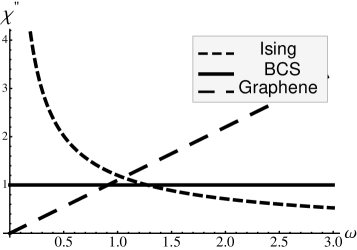
Figure 1: Illustration of the imaginary part of the pair susceptibility, comparing the relevant (Ising class), marginal (BCS case) and irrelevant (graphene class). The scaling exponent $\alpha_{p}=\frac{2-\eta_{p}}{z}$ is respectively $0<\alpha_{p}<1,\alpha_{p}=0,\alpha_{p}<0$. For the Ising class, the magnitude of the imaginary part of the pair susceptibility becomes larger and larger as one lowers the frequency. For the BCS case, the magnitude stays constant as the frequency is changed. For the graphene class, the magnitude decreases to zero in the low frequency infrared region.

According to general conformal wisdoms, the pair operator is called irrelevant when $\alpha_{p}<0$ such that $\chi"$ increases with frequency, relevant when $0<\alpha_{p}<1$ when $\chi^{\prime\prime}$ decreases with frequency and marginal when $\alpha_{p}=0$, such that $\chi^{\prime\prime}_{p}$ is frequency independent, see Fig 1. From this scaling perspective, the Fermi liquid pair operator is just the special marginal case, and the BCS superconductor with its logarithmically running coupling constant falls quite literally in the same category as the asymptotically free quantum chromo dynamics in 3+1D and the Kondo effect. Another familiar case is the pair susceptibility derived from the ’Dirac fermions’ of grapheneUchoa and Neto (2007); Kopnin and Sonin (2008) and transition metal dichalcogenidesNeto (2001); Uchoa et al. (2005) characterized by $\alpha_{p}=-1$: in this ’irrelevant case’ one needs a finite glue interaction to satisfy the instability criterium.

The scaling behavior of the free fermion case is special and the pair operator in a general conformal fermionic state can be characterized by a scaling dimension that is any real number smaller than one. Obviously, the interesting case is the relevant one where $\alpha_{p}>0$ (Fig.1). Let us here consider the zero temperature gap equation. In Eq. (6) we have already fully specified $\chi^{\prime\prime}_{p}$ in the critical state. However, due to the zero temperature condensate the scale invariance is broken and the low frequency part of $\chi^{\prime\prime}_{p}$ will now be dominated by an emergent BCS spectrum including a $s-$ or $d-$wave gap, Bogoliubov fermions and so forth. This will be discussed in detail in section V. Let us here introduce the gap in the BCS style by just assuming that the imaginary part of the pair susceptibility vanishes at energies less than $\Delta$. Under this assumption the gap equation becomes,

$$1-2g\int_{\Delta}^{2\omega_{B}}\frac{d\omega}{\omega}\frac{Z^{\prime\prime}\sin((\pi/2)\alpha_{p})}{\omega^{(2-\eta_{p})/z}}=0,$$ (9)

evaluating the integral this becomes our ’quantum critical gap equation’ ,

$$\Delta=2\omega_{B}\left({1+\frac{1}{\tilde{\lambda}}\left(\frac{2\omega_{B}}{\omega_{c}}\right)^{\alpha_{p}}}\right)^{-\frac{1}{\alpha_{p}}},$$ (10)

with

$$\tilde{\lambda}=2\lambda\frac{1-\alpha_{p}}{\alpha_{p}},$$ (11)

and $\lambda\equiv g/\omega_{c}$. The numerator $(1-\alpha_{p})$ in $\tilde{\lambda}$ comes from the normalization constant $Z^{\prime\prime}$, while the denominator $\alpha_{p}$ from integrating over $\omega$. Notice that $\lambda$ has the same meaning of a conventional, say, dimensionless electron-phonon coupling constant. The dimensionful coupling constant $g$ parametrizes the interaction strength between microscopic electrons and -lattice vibrations, and $\omega_{c}$ has the same status as the Fermi-energy in a conventional metal as the energy scale that is required to balance $g$. We argued earlier that $\omega_{c}$ is of order of the bare Fermi energy and therefore it make sense to use here values for e.g. the electron-phonon coupling constant as quoted in the LDA literature. Notice however that for a given $\lambda$ the effective coupling constant $\tilde{\lambda}$ that appears in Eq. (10) is decreasing when $\alpha_{p}$ is becoming more relevant, i.e. when $\alpha_{p}\rightarrow 1$. From the frequency integral $\int d\omega\omega^{-(1+\alpha_{p})}$, one would anticipate that the gap would increase for a more relevant pair susceptibility. The unitary condition imposes however an extra condition on the pair susceptibility. These two compensating effects lead to the important result that the gap is rather sensitive to the relevancy of the pair susceptibility. All what really matters is whether the pair susceptibility is relevant rather than marginal or irrelevant, and the degree of the relevancy is remarkably unimportant.

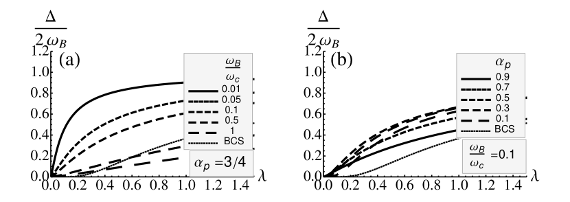
Figure 2: (a)The ratio of gap to retardation frequency $\Delta/(2\omega_{B})$ as a function of glue strength $\lambda$ for various retardation ranges $\omega_{B}/\omega_{c}$ with fixed scaling dimension $\alpha_{p}=3/4$. (b)The same plot, but with fixed retardation $\omega_{B}/\omega_{c}=0.1$ and various scaling dimensions $\alpha_{p}$. The dotted lines are the standard BCS result.

Eq.(10) is a quite different gap equation than the BCS one with its exponential dependence on the coupling $\lambda$. The multiplicative structure associated with the Fermi-liquid is scaling wise quite special, while Eq. (10) reflects directly the algebraic structure rooted in scale invariance. The surprise is that retardation acts quite differently when power laws are ruling. In Fig. (1) we show the dependence of the $\Delta/\omega_{B}$ ratio on the coupling constant $\lambda$, both for different Migdal parameters and fixed $\alpha_{p}$, as well as for various scaling dimensions and the Migdal parameter fixed. The comparison with the BCS result shows that drastic changes happen already for small scaling dimensions $\alpha_{p}$ especially in the small $\lambda$ regime. Our equation actually predicts that the gap to glue frequency ratio becomes of order one alrady for couplings that are as small as $\lambda=0.1$ when the Migdal parameter is small. To place this in the context of high Tc superconductivity, let us assume that the pairing glue in the cuprates is entirely rooted in the ’glue peak’ at $\omega_{B}\sim 50$meV that is consistently detected photoemission, tunneling spectroscopy and optical spectroscopyLee et al. (2006); Damascelli et al. (2003); van Heumen et al. . The electronic cut-off in the cuprates is likely of order $\omega_{c}=0.5$ eV such that the Migdal parameter $\omega_{B}/\omega_{c}\simeq 0.1$. A typical gap value is $40$ meV and we read off Fig. 1 that we need $\lambda=0.45$ or $0.43$ for $\alpha_{p}=3/4,1/4$ while using the BCS equation $\lambda=1.1$! Taking this serious implies that in principle one needs no more than a standard electron-phonon coupling to explain superconductivity at a high temperature in cuprate superconductors. Of course this does not solve the problem: although one gets a high Tc for free it still remains in the dark how to form a fermionic quantum critical state with a high cut-off energy, characterized by a relevant pair susceptibility.

Eq.(10) is also very different from the gap equations obtained in the previous attempts to apply scaling theory to superconducting transition by BalatskyBalatsky (1993), SudboSudbo (1995) and Yin and ChakravartyYin and Chakravarty (1996). A crucial property of their results is that even in the relevant case one needs to exceed a critical value for $\lambda$ to find a superconducting instability. The present scaling theory is in this regard a more natural generalization of BCS theory, where the standard BCS is just the ’marginal end’ of the relevant regime where the Cooper instability cannot be avoided for attractive interactions. The previous approaches Balatsky (1993); Sudbo (1995); Yin and Chakravarty (1996) start by considering the single particle spectral function, generalizing its analytic structure from simple poles to branch cuts. This way of thinking stems from the Fermi-liquid type assumption that the single particle Green’s function is the only primary operator of the system, and all the higher point functions are secondary operators, to be determined by the single particle Green’s function. But for critical systems, such assumptions are generally not to satisfied. It is well known for example from the AdS/CFT correspondence, that the four-point functions of strongly interacting conformal fields are much more complex than the combination of two-point functionsMuck and Viswanathan (1998); Freedman et al. (1999); D’Hoker and Freedman (1998a); Liu (1998); D’Hoker and Freedman (1998b); D’Hoker et al. (1999); Chalmers and Schalm (1998, 1999). Our basic assumption is that the pair susceptibility is by itself a primary operator subjected to conformal invariance which is the most divergent operator at the critical point.

III Determining the transition temperature.

Let us now turn to finite temperatures. A complicating fact is that temperature breaks conformal invariance, since in the euclidean formulation of the field theory its effect is that the periodic imaginary time acquires a finite compactification radius $R_{\tau}=\hbar/k_{B}T$. The pair susceptibility therefore acquires the finite size scaling formSachdev (1999)

$$\chi(\omega)\equiv\chi({\vec{q}}=0,\omega)=ZT^{-(2-\eta_{p})/z}\Phi\left(\frac{\omega}{T}\right),$$ (12)

where $\Phi$ is a universal scaling function and $Z$ is a UV renormalization constant, while $\eta_{p}$ and $z$ are the anomalous scaling dimension of the pair operator and the dynamical critical exponent, respectively. At zero temperature this turns into the banch cut as shown in Eq.(6), while in the opposite high temperature or hydrodynamical regime ($\hbar\omega<<k_{B}T$) it takes the formSachdev (1999)

$$\chi(\omega)=Z^{\prime}T^{-(2-\eta_{p})/z}\frac{1}{1-i\omega\tau_{rel}},$$ (13)

where $\tau_{rel}\approx\hbar/k_{B}T$. The crossover from the hydrodynamical- (Eq. 6) to the high frequency coherent regime(Eq. 13) occurs at an energy $\sim k_{B}T$. The superconducting transition temperature is now determined by the gap equation through $1-g\chi^{\prime}_{\rm ret}(k_{B}T_{c})=0$. The problem is that $\chi^{\prime}_{ret}$ is via the Kramers-Kronig transformation largely set by the cross-over regime in $\chi^{\prime\prime}_{p}$. One needs the full solutions of the CFT’s to determine the detailed form of $\Phi$ in this crossover regime and these are not available in higher dimensions.

In 1+1D these are however completely determined by conformal invariance, and for our present purposes these results might well represent a reasonable model since the gap equation is only sensitive to rather generic features of the cross-over behavior. Given the exponents $\eta_{p}$ and $z$, the exact result for the finite temperature $\chi^{\prime\prime}$ in 1+1D is well known and can be easily derived from the universal two-point correlator at an imaginary time $\tau$Sachdev (1999)

$$C(x,\tau)={\tilde{Z}}\frac{T^{2s}}{\left(\sin[\pi T(\tau-ix)]\sin[\pi T(\tau+ix)]\right)^{s}},$$ (14)

with $1-2s=\frac{2-\eta_{p}}{2z}$. The analytical continuation to real time $\tau\to it$ yields the real time two-point correlation function

$$C(x,t)={\tilde{Z}}\frac{T^{2s}}{\left(i\sinh[\pi T(t-x)]i\sinh[\pi T(t+x)]\right)^{s}},$$ (15)

with a Fourier transform corresponding to the dynamic structure factor

$$S(k,\omega)=\int_{-\infty}^{\infty}dx\int_{-\infty}^{\infty}dtC(x,t)e^{-i(kx-\omega t)}.$$ (16)

A convenient way to perform the Fourier transform is by factorizing $C(x,t)$ into left-moving and right-moving modes, $C(x,t)=C_{-}(t-x)C_{+}(t+x)$, to subsequently integrate over $t\pm x$. The result is

$$S(k,\omega)=Ze^{\frac{\omega}{2T}}\frac{1}{T^{2(1-2s)}}B(s+i\frac{\omega+k}{4\pi T},s-i\frac{\omega+k}{4\pi T})B(s+i\frac{\omega-k}{4\pi T},s-i\frac{\omega-k}{4\pi T}),$$ (17)

where $B$ is the beta function, and the overall numerical coefficient $Z=2^{4s-3}\pi^{2(s-1)}{\tilde{Z}}$. The fluctuation-dissipation theorem

$$S(k,\omega)=\frac{2}{1-e^{-\omega/T}}\chi^{\prime\prime}(k,w)$$ (18)

then yields the imaginary part of the pair susceptibility,

$$\chi^{\prime\prime}(k,\omega)=Z\frac{\sinh(\frac{\omega}{2T})}{T^{2(1-2s)}}B(s+i\frac{\omega+k}{4\pi T},s-i\frac{\omega+k}{4\pi T})B(s+i\frac{\omega-k}{4\pi T},s-i\frac{\omega-k}{4\pi T}),$$ (19)

The temperature and frequency dependencies of this function for $k=0$ are illustrated in Fig.(3). Indeed $\chi^{\prime\prime}(\omega)\to 0$ in a linear fashion with $\omega$ with a slope set by $1/T$, while for $\omega>>T$ the temperature dependence drops out, recovering the power law. The crossover occurs at $\omega\simeq 2k_{B}T/\hbar$ where $\chi^{\prime\prime}(\omega)$ has a maximum. In the absence of retardation, the real part can be computed from the Kramers-Kronig transform,

$$\chi^{\prime}(k,\omega)=\frac{Z^{\prime}}{T^{2(1-2s)}} \left(\frac{-i\pi}{s-i\frac{\omega+k}{4\pi T}}\frac{\sin(2s\pi-\frac{ik}{2T})}{\sinh(\frac{k}{2T})}\frac{\Gamma(2s)\Gamma(2s-\frac{ik}{2\pi T})}{\Gamma(1-\frac{ik}{2\pi T})}\>{}_{3}F_{2}(2s,s-i\frac{\omega+k}{4\pi T},2s-\frac{ik}{2\pi T};1+s-i\frac{\omega+k}{4\pi T},1-\frac{ik}{2\pi T};1)\right.$$ (20)

$$+\left.(k\rightarrow-k)\right)$$ ,

where $F$ is the generalized hypergeometric function. We did not manage to obtain an analytic form for the real part when retardation is included, and we use numerical results instead.

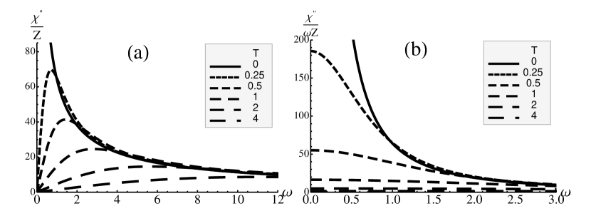
Figure 3: (a)Illustration of the imaginary part of the pair susceptibility $\chi^{\prime\prime}(k=0,\omega,T)$ divided by the overall numerical factor $Z$, as a function of frequency $\omega$ for various temperatures. Here we’ve chosen $\alpha_{p}=3/4$, so $s=5/16$. (b) The same plot, but $\chi^{\prime\prime}$ is further divided by $\omega$. At zero temperature one has the power law scaling form. At finite temperature $\chi^{\prime\prime}(\omega)$ goes to zero, as $\omega$ goes to zero ($\chi^{\prime\prime}(\omega)/\omega\to{\rm constant}$, as $\omega\to 0$), and approaches the same power law behavior at large frequency. As one increases temperature, the maximum of $\chi^{\prime\prime}(\omega)$ goes down, and the corresponding $\omega_{max}$ shifts to larger frequency.

When temperature goes to zero the limiting form of the beta function becomes,

$$\lim_{u\to\infty}B(s+iu,s-iu)=\frac{2\pi}{\Gamma(2s)}e^{-\pi u}u^{2s-1},$$ (21)

and the imaginary part of the pair susceptibility Eq. (19) acquires the power law form

$$\chi^{\prime\prime}(\omega)=\frac{2\pi^{2}(4\pi)^{\alpha_{p}}}{[\Gamma(2s)]^{2}}Z\frac{1}{\omega^{\alpha_{p}}}.$$ (22)

Comparing this with Eq.(7) yields the normalization factor in terms of the cut-off scale

$$Z=\frac{[\Gamma(2s)]^{2}(1-\alpha_{p})}{2\pi^{2}(4\pi)^{\alpha_{p}}\omega_{c}^{1-\alpha_{p}}}.$$ (23)

Combining Eq.’s (1),(2),(19),(23), we obtain the equation determining the critical temperature,

$$1-{\cal C}^{\prime}\lambda\left(\frac{2\omega_{B}}{\omega_{c}}\right)^{-\alpha_{p}}\left(\frac{T_{c}}{2\omega_{B}}\right)^{-\alpha_{p}}{\cal F}\left(\frac{2\omega_{B}}{T_{c}}\right)=0,$$ (24)

where

$${\cal F}(y)=\int_{0}^{y}\frac{dx}{x}\sinh(\frac{x}{2})\left({\rm B}(s+i\frac{x}{4\pi},s-i\frac{x}{4\pi})\right)^{2},$$ (25)

and $x=\omega/T$. The overall coefficient is

$${\cal C}^{\prime}=\frac{[\Gamma(2s)]^{2}(1-\alpha_{p})}{\pi^{2}(4\pi)^{\alpha_{p}}}.$$ (26)

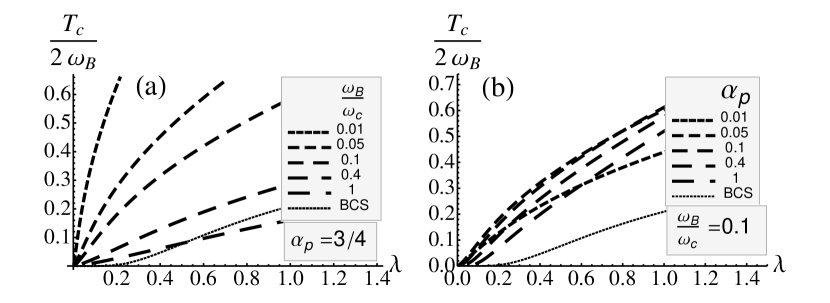
Figure 4: (a)The ratio of transition temperature to retardation frequency $T_{c}/(2\omega_{B})$ as a function of glue strength $\lambda$ for various retardation ranges $\omega_{B}/\omega_{c}$, with scaling dimension fixed $\alpha_{p}=3/4$. (b)The same plot, but fix the retardation $\omega_{B}/\omega_{c}=0.1$ while varying the scaling dimensions $\alpha_{p}$. The dotted lines are the standard BCS result. The magnitude and dependence on glue strength and retardation are all similar to those of the gap.

We plot in Fig.(4) the ratio of $T_{c}$ to retardation frequency as function of glue strength, retardation and the scaling dimensions. One infers that the behavior of $T_{c}$ is very similar to that of the zero temperature gap, plotted in Fig. (2). We observe that they are of the same order of magnitude $T_{c}\sim\Delta$, and this can be understood from the behavior of $\chi^{\prime\prime}/\omega$ plotted in Fig.(3b). Since the large frequency behavior of $\chi^{\prime\prime}(\omega)/\omega$’s are the same for different temperatures, all what matters is the low frequency part. The gap imposes a cut-off for the zero temperature $\chi^{\prime\prime}(\omega)/\omega$, and its value is determined such that the area under this curve including the low frequency cut-off, is the same as the area under the curve corresponding to $T_{c}$ without a cut-off: by inspecting Fig.(3b) one infers directly that the gap and $T_{c}$ will be of the same order. The same logic is actually at work in the standard BCS case. The finite temperature Fermi gas susceptibility is $\chi^{\prime\prime}(\omega)=\frac{1}{2E_{F}}\tanh(\frac{1}{4}\beta\omega)$ Allen (1980), and the familiar $T_{c}$ equation follows,

$$1-\lambda\int_{0}^{2\omega_{B}}\frac{d\omega}{\omega}\tanh(\frac{1}{4}\beta\omega)=0,$$ (27)

such that $T_{c}\simeq 1.14\omega_{B}e^{-1/\lambda}$, of the same order as the BCS gap $\Delta=2\omega_{B}e^{-1/\lambda}$. Now the effect of temperature is encoded in the $\tanh$ function. Although the Fermi-gas is not truly conformal, It is easy to check that this ’fermionic’ $\tanh$ factor adds a temperature dependence to the $\chi^{\prime\prime}$ that is nearly indistinguishable from what one obtains from the truly conformal marginal case that one obtains by setting $s=1/2$ in Eq. (19).

We notice that conformal invariance imposes severe constraints on the finite temperature behavior of the pair susceptibility, thereby simplifying the calculation of $T_{c}$. In the $1+1$-dimensional ’model’ nearly everything is fixed by conformal invariance. The only free parameters that enter the calculation are the scaling dimension $\alpha_{p}$, the cut-off scale $\omega_{c}$ and the glue quantities. As we will now argue the situation is actually much less straightforward for the zero temperature gap because this involves a detailed knowledge of the crossover to the physics of the superconductor ruling the low energy realms.

IV The gap equation: gluing a quantum critical metal to a BCS superconductor.

It is part of our postulate that when superconductivity sets in BCS ’normalcy’ returns at low energies in the form of the sharp Bogoliubov fermions and so forth. Regardless the critical nature of the normal state, the scale invariance gets broken by the instability where the charge 2e Cooper pairs form, and this stable fixed point also dictates the nature of the low lying excitations. However, we are dealing with the same basic problem as in the previous section: in the absence of a solution to the full, unknown theory it is impossible to address the precise nature of the cross-over regime between the BCS scaling limit and the critical state at high energy. This information is however required to further improve the gap equation Eq. (10) of section II that was derived by crudely modeling $\chi^{\prime\prime}$ in the presence of the superconducting condensate.

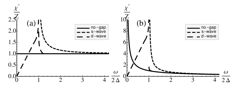
Figure 5: Illustration of the imaginary part of the pair susceptibility without a gap and in the presence of an $s$- and $d$- wave gap, for (a) the BCS case, and (b) the quantum critical case (here we’ve plotted using the parameter $\alpha_{p}=3/4$). In the absence of gap, $\chi^{\prime\prime}$ is a constant (for BCS) or has a simple power law behavior (for critical fermions). In the presence of a s-wave gap, the states below the gap are gapped out and there is a power law singularity right above the gap. When there is a d-wave gap, the low frequency part (way below the gap) is governed by a Dirac cone structure, thus a linear susceptibility, while near the gap a van Hove singularity is at work, leading to logarithmic divergences on both sides. The high frequency region for both s- and d-wave gap goes over to the case without a gap.

So much is clear that the crossover scale itself is set by the gap magnitude $\Delta$. However, assuming that this affair has dealings with e.g. optimally doped cuprate superconductors, we can rest on experimental information: in optimally doped cuprates at low temperatures the coherent Bogoliubov fermions persist as bound states all the way to the gap maximum. Up to these energies it is therefore reasonable to assume that $\chi^{\prime\prime}_{p}$ is determined by the bare fermion loops, and this regime has to be smoothly connected to the branch cut form of the $\chi^{\prime\prime}_{p}$ at higher energies. This implies that the standard BCS gap singularities have to be incorporated in our zero temperature pair susceptibility. As a final requirement, the pair susceptibility has to stay normalized according to Eq. (4), which significantly limits the modelling freedom.

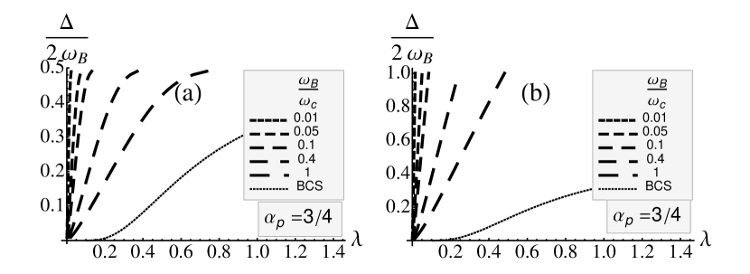
Figure 6: The ratio of the gap to retardation $\Delta/(2\omega_{B})$ as a function of the glue strength $\lambda$, for various retardation ranges, with (a) a s-wave gap and (b) a d-wave gap. Here we’ve chosen $\alpha_{p}=3/4$. The dotted lines are the standard BCS result. The dependence on glue strength and and retardation is similar but the magnitude of the gap is much enhanced compared to the previous treatment of gap as a simple IR cutoff. The d-wave case is enhanced even more.

Let us first consider the case of an isotropic s-wave gap singularity. The high frequency modes are still critical, and therefore the high frequency limit of the imaginary part of the pair susceptibility is determined by,

$$\lim_{\omega\to\infty}\chi^{\prime\prime}(\omega,\Delta,T=0)=\frac{\cal A}{\omega^{\alpha_{p}}}.$$ (28)

In the presence of the superconducting condensate, the low energy modes below the gap have their energy raised above the gap, since we require $\chi^{\prime\prime}(\omega<\Delta,\Delta,T=0)=0$. The spectral weight is conserved according to Eq. (4), and since we assumed that the Bogoliubov excitations of the BCS fixed point survive at energies of order of the gap we need to incorporate a BCS s-wave type power law divergence right above the gap in the imaginary part of the pair susceptibility. The simplest function satisfying these conditions is,

$$\chi^{\prime\prime}(\omega,\Delta)={\cal A}\frac{1}{\omega^{\alpha_{p}}}\left(\frac{\omega}{\sqrt{\omega^{2}-(2\Delta^{2})}}\right)^{1+\alpha_{p}}\Theta(\omega-2\Delta),$$ (29)

with ${\cal A}=(1-\alpha_{p})\omega_{c}^{-(1-\alpha_{p})}$ (see Fig.5b). We notice in passing that the BCS gap corresponds to the case $\alpha_{p}=0$,

$$\chi_{\rm BCS}^{\prime\prime}(\omega,\Delta)=\frac{1}{2E_{F}}\frac{\omega}{\sqrt{\omega^{2}-(2\Delta)^{2}}}\Theta(\omega-2\Delta).$$ (30)

The quantum critical gap equation for the s-wave superconductor now becomes,

$$1-2(1-\alpha_{p})\lambda\left(\frac{2\omega_{B}}{\omega_{c}}\right)^{-\alpha_{p}}\left(\frac{\Delta}{\omega_{B}}\right)^{-\alpha_{p}}\int_{1}^{\frac{\omega_{B}}{\Delta}}\frac{dx}{(x^{2}-1)^{(1+\alpha_{p})/2}}=0.$$ (31)

Turning to the d-wave case the gap equation becomes necessarily a bit more complicated since we have to account for massless Bogolubiov fermions. At low frequencies $\omega<<2\Delta$ the pair susceptibility is now governed by free fermion loops and the Dirac-cone structure in the spectrum leads to a linear frequency dependence in the pair susceptibility, $\chi^{\prime\prime}(\omega)={\cal A}_{1}\omega$. Near the gap, a logarithmic divergence is expected due to the Van Hove singularity, and therefore $\chi^{\prime\prime}(\omega)={\cal A}_{2}\log\frac{q_{c}+\sqrt{2\Delta-\omega+q_{c}^{2}}}{-q_{c}+\sqrt{2\Delta-\omega+q_{c}^{2}}}$ for $\omega<2\Delta$, while $\chi^{\prime\prime}(\omega)={\cal A}_{3}\log\frac{q_{c}+\sqrt{\omega-2\Delta+q_{c}^{2}}}{-q_{c}+\sqrt{\omega-2\Delta+q_{c}^{2}}}$ for $\omega>2\Delta$, with $q_{c}$ a cutoff. When the frequency is high compared to the gap scale, the pair susceptibility has the scaling form $\chi^{\prime\prime}(\omega)={\cal A}_{4}\omega^{-\alpha_{p}}$. Matching these regimes at $2\Delta-\omega_{1}$ and $2\Delta+\omega_{2}$, with $0<\omega_{1}<2\Delta$ and $0<\omega_{2}<2\omega_{B}-2\Delta$, and assuming continuity of the pair susceptibility both below and above the gap (see Fig. 5b), we arrive at the gap equation for the d-wave case,

$$\frac{1}{2g}={\cal A}_{1}(2\Delta-\omega_{1}) + {\cal A}_{2}\frac{q_{c}^{2}}{2\Delta}\int_{0}^{\omega_{1}/q_{c}^{2}}\frac{dx}{1-xq_{c}^{2}/(2\Delta)}\log\frac{1+\sqrt{x+1}}{-1+\sqrt{x+1}}$$ (32)

$$+ {\cal A}_{3}\frac{q_{c}^{2}}{2\Delta}\int_{0}^{\omega_{2}/q_{c}^{2}}\frac{dx}{1+xq_{c}^{2}/(2\Delta)}\log\frac{1+\sqrt{x+1}}{-1+\sqrt{x+1}}+\frac{{\cal A}_{4}}{\alpha_{p}}\left[(2\Delta+\omega_{2})^{-\alpha_{p}}-(2\omega_{B})^{-\alpha_{p}}\right].$$

This contains a number of free parameters that are partially constrained by the spectral weight conservation. This however does not suffice to determine the gap uniquely. In the following we will make further choice of the parameters, to plot the gap. We choose the scaling dimension $\alpha_{p}=3/4$, and the cut-off in the logarithm to be of order the square root of the gap, say $q_{c}/\sqrt{2\Delta}=3$, the width of the logarithmic region to be 20 percent of the magnitude of the gap on both sides of the gap, that is $\omega_{1}/(2\Delta)=\omega_{2}/(2\Delta)=0.2$, the coefficient of the high frequency part ${\cal A}_{4}=1/(4\omega_{c}^{3/4})$, and further define $\omega_{1}/q_{c}^{2}=\omega_{2}/q_{c}^{2}\equiv a$, $b\equiv\int_{0}^{a}dx\log\frac{1+\sqrt{x+1}}{-1+\sqrt{x+1}},c\equiv\log\frac{1+\sqrt{a+1}}{-1+\sqrt{a+1}},d\equiv\frac{4\times 1.2^{1/4}-1.2^{-3/4}\times 9b/c}{0.32+7.2b/c}$, thus the corresponding d-wave gap equation reads,

$$1-\frac{1}{2}\lambda\left(\frac{2\omega_{B}}{\omega_{c}}\right)^{-\frac{3}{4}}\left(\frac{\Delta}{\omega_{B}}\right)^{-\frac{3}{4}}\left(0.8d\right. + 7.2\frac{d}{c}\int_{0}^{a}\frac{dx}{1-9x}\log\frac{1+\sqrt{x+1}}{-1+\sqrt{x+1}}$$ (33)

$$+ 9\frac{1.2^{-\frac{3}{4}}}{c}\int_{0}^{a}\frac{dx}{1+9x}\log\frac{1+\sqrt{x+1}}{-1+\sqrt{x+1}}+\frac{4}{3}(1.2^{-\frac{3}{4}}-(\frac{\Delta}{\omega_{B}})^{\frac{3}{4}})\left.\right)=0,$$

We plot in Fig.(6) the behavior of the gap function in the s- and d-wave cases, to be compared with the outcomes Fig. (2) of the approach taken in section II where the gap simply entered as an IR cut-off scale, Eq. (9). One can see that in both cases the magnitude of the gap is enhanced by treating the singularity more carefully, while in the d-wave case this enhancement is even more pronounced than in the s-wave case. These effects can be understood in terms of the redistribution of the spectral weight, since the low frequency part is enhanced by the factor $1/\omega$ in the Kramers-Kronig frequency integral. The dependence of the gap on the glue strength and retardation does however not change significantly compared to what we found in section II, which can be understood from the fact that the gap depends on the combination $\lambda(2\omega_{B}/\omega_{c})^{-\alpha_{p}}$. One also notices in Fig.(6) that the magnitude of the gap saturates already at small $\lambda$ for modest retardation. This is an artifact of the modeling. In real system the power law (s-wave) or logarithmic (d-wave) spectral singularities will be damped (see e.g. Dzyaloshinskii (1996); Irkhin et al. (2001, 2002); Rubtsov et al. (2009)), and the endpoints at finite $\lambda$ in Fig.(6) will turn into smooth functions..

The gap to $T_{c}$ ratio is expected to be a number order unity number. However, it is quite sensitive to the details of the crossover regime between the high frequency critical behavior and the low frequency superconducting behavior as of relevance to the zero temperature gap. Numerically evaluating Eq.’s (24,31,33) we obtain gap to $T_{c}$ ratio’s as indicated in Fig. (7). Different from the Migdal-Eliasbergh case we find that these ratio’s are rather strongly dependent on both the Migdal- and the coupling parameter, while the ratio becomes large for small coupling, in striking contrast with conventional strong coupling superconductivity. Invariably we find the ratio to be larger than the weak coupling BCS case, reflecting the strongly dissipative nature of quantum critical states at finite temperature that plays apparently a similar role as the ’pair-breaking’ phonon heat bath in conventional superconductors.

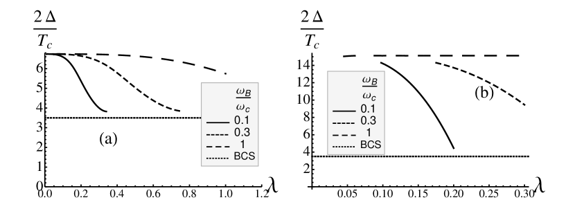
Figure 7: (a)The gap to $T_{c}$ ratio $2\Delta/T_{c}$ as a function of glue strength $\lambda$ for various retardation ranges $\omega_{B}/\omega_{c}$ with fixed scaling dimension $\alpha_{p}=3/4$, for s-wave pairing. The dotted line is the standard BCS result, where $2\Delta/T_{c}=3.5$. (b) The same plot for d-wave pairing. The gap to $T_{c}$ ratio decreases with increasing glue strength and retardation for both s- and d-wave gap. The ratios for different retardation ranges approach the same constant as $\lambda\to 0$.

V Away from the critical points: the superconducting dome versus $T^{*}$.

Figure 8: Illustration of the imaginary part of the pair susceptibility away from the critical point. For $\omega>T^{*}$, it has the critical scaling behavior, while for $\omega<T^{*}$, it retains the BCS form. $T^{*}$ is the cross-over scale. The effective mass $m^{*}$ is identified as the magnitude of the imaginary part of the pair susceptibility in the BCS region. The gap $\Delta$ acts as a low energy cut-off, and the retardation $2\omega_{B}$ as a high energy cut-off. When $T^{*}$ lies between $\Delta$ and $2\omega_{B}$, as is the case shown above, both the critical modes and Fermi liquid modes contribute. When $\Delta>T^{*}$, only the critical modes contribute. When $2\omega_{B}<T^{*}$, only the Fermi liquid modes contribute.

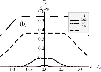
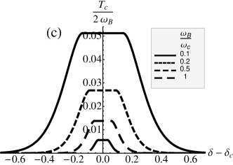
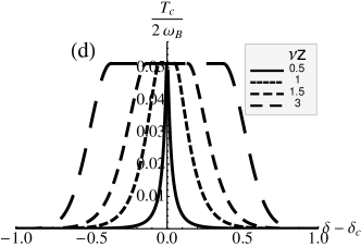
Figure 9: The ratio of $T_{c}$ to retardation as a function of the distance away from criticality (a) for various scaling exponent $\alpha_{p}$’s with $\lambda=0.06,\omega_{B}/\omega_{c}=0.1,\nu z=3/2$, (b) for various glue strength $\lambda$’s with $\omega_{B}/\omega_{c}=0.1,\nu z=3/2,\alpha_{p}=5/6$. (c) for various retardation over cut-off $\omega_{B}/\omega_{c}$’s with $\lambda=0.06,\nu z=3/2,\alpha_{p}=5/6$. (d) for various inverse Grüneisen exponent $\nu z$’s with $\lambda=0.06,\omega_{B}/\omega_{c}=0.1,\alpha_{p}=5/6$.

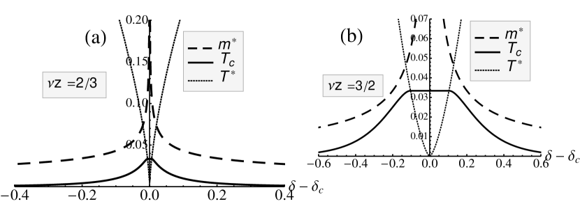
Figure 10: (a):The superconducting transition temperature $T_{c}$ as a function of the distance from the critical point, for given crossover temperature $T^{*}$ and retardation $\omega_{B}$. The parameters are chosen as $z=2,\nu=1/3,\eta_{p}=1,\lambda=0.05,\omega_{B}/\omega_{c}=0.1$. (b):The same plot for a different set of parameters $z=3,\eta=0.5,\nu=1/2,\lambda=0.05,\omega_{B}/\omega_{c}=0.1$. In-between the two points $\delta_{c}\pm{\tilde{\delta}}$, at which the transition temperature coincides with the cross-over temperature $T_{c}(\delta_{c}\pm{\tilde{\delta}})=T^{*}(\delta_{c}\pm{\tilde{\delta}})$, the critical temperature remains constant. For $T^{*}>2\omega_{B}$, $T_{c}$ decays exponentially. The schematic behavior of the effective mass $m^{*}$ is also included. It diverges when approaching the critical point.

Our scaling theory yields a simple and natural explanation for the superconducting domes surrounding the QCP’s. This is usually explained in the Moriya-Herz-Milles frameworkHertz (1976); Millis (1993); Moriya and Takimoto (1995); Pepin (2005) that asserts that the critical fluctuations of the bosonic order parameter turn into glue with singular strength while the Fermi-liquid is still in some sense surviving. We instead assert that the glue is some external agent (e.g., the phonons but not necessarily so) that is blind to the critical point, but the fermionic criticality boosts the SC instability at the QCP according to Eq. (10). By studying in detail the variation of the SC properties in the vicinity of the QCP it should be possible to test our hypothesis. The data set that is required is not available in the literature and let us present here a crude sketch of what can be done. In at least some heavy fermion systemsCusters et al. (2003) a rather sudden cross-over is found between the high temperature critical state and a low temperature heavy Fermi-liquid, at a temperature $T^{*}\sim|\delta-\delta_{c}|^{\nu z}$, with $\nu$ behaving like a correlation length exponent $\xi\sim|\delta-\delta_{c}|^{-\nu}$ as function of the zero temperature tuning parameter $\delta$. Moving away from the QPT this means for the SC instability that an increasingly larger part of the frequency interval of $\chi^{\prime\prime}$ below $\omega_{B}$ is governed by the Fermi-liquid ’flow’ with the effect that $T_{c}$ decreases. We can crudely model this by asserting that the imaginary part of the pair susceptibility acquires the critical form for $\omega>T^{*}$ and the Fermi-liquid form for $\omega<T^{*}$, while we impose that it is continuous at $\omega=T^{*}$. This model has the implication that the magnitude of $\chi^{\prime\prime}$ in the Fermi-liquid regime is determined by $T^{*}$ and $\eta_{p}$ and we find explicitly that $N_{0}\propto m^{*}\propto|\delta-\delta_{c}|^{-\nu(2-\eta_{p})}$. We notice that this should not be taken literally, since this cross-over behavior can be a priori more complicated. In fact, from thermodynamic scaling it is known Zhu et al. (2003); Zaanen and Hosseinkhani (2004) that $m^{*}\sim|\delta-\delta_{c}|^{\nu(d-z)}$. Fig. (8) would imply that $\alpha_{p}=1-d/z$. This is not implied by scaling.

Given these assumptions, the gap equation away from the quantum critical point becomes,

$$1-2g\left(\int_{\Delta}^{T^{*}}\frac{d\omega}{\omega}\chi^{\prime\prime}_{\rm BCS}(\omega)+\int_{T^{*}}^{2\omega_{B}}\frac{d\omega}{\omega}\chi^{\prime\prime}_{\rm crit}(\omega)\right)=0$$ (34)

We are interested in the superconducting transition temperature, which has been shown in the previous section to be approximately the gap magnitude $T_{c}\simeq\Delta$. The imaginary part of the pair susceptibility in the critical region has still the power law form $\chi^{\prime\prime}_{\rm crit}(\omega)=Z^{\prime\prime}\sin(\alpha_{p}\pi/2)\omega^{-\alpha_{p}}$, while in the BCS region it is a constant determined by continuity at $\omega=T^{*}$ and therefore $\chi^{\prime\prime}_{\rm BCS}(\omega)=Z^{\prime\prime}\sin(\alpha_{p}\pi/2)(T^{*})^{-\alpha_{p}}$.

Consequently we find in the regime $T_{c}<T^{*}<2\omega_{B}$ the solution for the gap equation,

$$T_{c}=2\omega_{B}x^{\nu z}\exp\left[\frac{1}{\alpha_{p}}\left(1-x^{\nu(2-\eta_{p})}-\frac{1}{\tilde{\lambda}}(\frac{2\omega_{B}}{\omega_{c}})^{\alpha_{p}}x^{\nu(2-\eta_{p})}\right)\right],$$ (35)

where $x^{\nu z}=T^{*}/(2\omega_{B})$. For $T^{*}<T_{c}$ a plateau is found since only the critical modes contribute to the pairing, while for $T^{*}>2\omega_{B}$ the BCS exponent takes over since only the (heavy) Fermi-liquid quasiparticles contribute having as a consequence,

$$T_{c}=2\omega_{B}\exp\left(-(\frac{2\omega_{B}}{\omega_{c}})^{\frac{2-\eta_{p}}{z}}\frac{x^{\nu(2-\eta_{p})}}{\alpha_{p}\tilde{\lambda}}\right).$$ (36)

The outcomes are illustrated in Fig. (9,10). One notices in all cases that the dome shapes are concave with a tendency for a flat ’maximum’. This is automatically implied by our starting assumptions. When $T_{c}$ is larger than $T^{*}$ only the critical regime is ’felt’ by the pairing instability and when this criterium is satisfied $T_{c}$ does not vary, explaining the flat maximum. When $T_{c}$ starts to drop below $T^{*}$ the superconductivity gets gradually depressed because the Fermi-liquid regime increasingly contributes. Eventually, far out in the ’wings’, one would still have superconductivity but with transition temperatures that become exponentially small. The domes reflect just the enhancement of the pairing instability by the critical fermion liquid relative to the Fermi-liquid.

The trends seen in Fig. 9 are easily understood. When the scaling dimension $\alpha_{p}$ is increasing, i.e. the pair operator is becoming more relevant, the maximum $T_{c}$ increases while not much happens with the width of the dome (Fig. 9a), for the simple reason that the critical metal becomes more and more unstable towards the superconductor. When the coupling strength $\lambda$ increases one finds in addition that the dome gets broader (Fig. 9b) because the ’contrast’ between Fermi-liquid and quantum critical BCS is becoming less, illustrating the surprise that especially weakly coupled quantum critical superconductors are much better than their traditional cousins. The same moral is found back when the Migdal parameter is varied (Fig. 9c), illustrating that at very strong retardation the differences are the greatest. Finally, in Fig. (9d) the evolution of the domes are illustrated when one changes the exponents relating $T^{*}$ to the reduced coupling constant. We find that the dome changes from a quite ’box like’ appearance to a ’peak’ pending the value of $\nu z$. The mechanism can be deduced from Fig. 10, comparing the situation that the quantum critical ’wedge’ is concave (fig. 10a, $\nu z<1$) with a convex wedge (fig. 10b, $\nu z>1$). Because $T^{*}$ is varying more slowly in he latter case with the reduced coupling constant, the quantum critical regime becomes effectively broader with the effect that the quantum critical BCS keeps control over a wider coupling constant range. The trends in Fig.’s (9, 10) are quite generic and it would be interesting to find out whether by systematical experimental effort these behaviors can be falsified or confirmed.

VI Spatial dependence of the pair susceptibility: upper critical field

Another experimental observable that should be quite revealing with regard to scaling behavior is the orbital limiting upper critical field. The orbital limiting field is set by the condition that the magnetic length becomes of order of the coherence length, and the latter relates to the ’time like’ $T_{c}$ merely by the dynamical critical exponent $z$. In more detail, assuming a gap of the form Rajagopal and Vasudevan (1966),

$$\Delta({\vec{r}})=\Delta_{0}\exp\left(-\frac{r^{2}}{2l^{2}}\right),$$ (37)

the linearized gap equation in the presence of an orbital limiting magnetic field becomes Abrikosov et al. (1963),

$$\frac{1}{{\Omega^{d-1}g}}=\int_{r_{0}}^{\infty}K_{0}(r,\beta)\exp\left(-\frac{r^{2}}{2l^{2}}\right)r^{d-1}dr,$$ (38)

where $\Omega^{d-1}$ is the volume of the $d-1$-dimensional unit sphere, $l$ is the magnetic length related to the field by $H={\phi_{0}}/({2\pi l^{2}})$ where $\phi_{0}=hc/e$, while $K_{0}(r,\beta)$ is the real space pair susceptibility, which is the Fourier transform of $\chi^{\prime}$Dias and Wheatley (1994); Schofield (1995). For free fermions, the real space pair susceptibility is (see eg. Dias and Wheatley (1994)),

$$K_{0}(r,\beta)=\left(\frac{k_{F}}{2\pi r}\right)^{d-1}\frac{1}{v_{F}^{2}\beta}\frac{1}{\sinh(\frac{2\pi r}{\beta v_{F}})},$$ (39)

with a power law behavior $K_{0}(r,\beta)\sim r^{-d}$ at short distances or low temperatures where $r<\beta v_{F}$, and an exponential decay at large distances or high temperature. Let us consider critical fermions at $T=0$, such that the pair susceptibility has the power law form $\chi(\omega)\sim\omega^{-(2-\eta)/z}$. The momentum dependence can be determined by replacing $\omega$ by $k^{z}$, such that $\chi(k)\sim k^{-(2-\eta)}$. It follows that the real space pair susceptibility has the power law form $K_{0}(r,T=0)\sim\int\chi(k)\exp(i{\vec{k}}\cdot{\vec{r}})d^{d}{\vec{k}}\sim r^{-(d-2+\eta_{p})}$. Associate with the retardation a short distance cutoff $r_{0}$, and assume a scaling $2\omega_{B}/\omega_{c}=(r_{0}/a_{c})^{-z}$, where $a_{c}$ is the lattice constant. The magnetic length acts as a long distance cutoff and therefore,

$$\frac{1}{{\Omega^{d-1}g}}=\int_{r_{0}}^{l}\frac{{\cal C}_{h}}{r^{d-2+\eta_{p}}}r^{d-1}dr,$$ (40)

with the normalization factor ${\cal C}_{h}\simeq 2z(1-\alpha_{p})\Omega^{-(d-1)}{\omega_{c}}^{-1}a_{c}^{-(2-\eta)}$, so that $(1/\Omega^{d-1})\int_{a_{c}}K_{\rm crit}(r)r^{d-1}dr\simeq\frac{1}{\omega_{c}}$, to give the right scale. The zero temperature upper critical field has then the same form as the one for $T_{c}$ except for the occurrence of $z$,

$$\frac{2\pi H_{c2}(0)}{\phi_{0}r_{0}^{-2}}\simeq\left({1+\frac{1}{\tilde{\lambda}}\left(\frac{2\omega_{B}}{\omega_{c}}\right)^{\alpha_{p}}}\right)^{-\frac{2}{2-\eta_{p}}},$$ (41)

and it follows,

$$\frac{2\pi H_{c2}(0)}{\phi_{0}a_{c}^{-2}}\simeq\left(\frac{T_{c}}{\omega_{c}}\right)^{2/z}.$$ (42)

In the BCS case one has $H_{c2}(0)/({\cal B}\phi_{0}k_{F}^{2})=(T_{c}/E_{F})^{2}$, with ${\cal B}\simeq 3.26$ for $d=3$ Helfand and Werthamer (1966). The moral is obvious: in Lorentz-invariant ($z=1$) systems the relation between $H_{c2}$ and $T_{c}$ is the same as for standard BCS, but when the normal state is governed by a universality class characterized by $z>1$, $H_{c2}(0)$ will be amplified for a given $T_{c}$ relative to conventional superconductors because $T_{c}/\omega_{c},T_{c}/E_{F}\ll 1$.

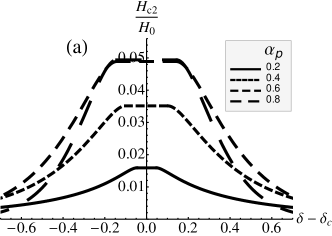
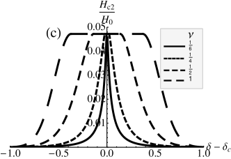
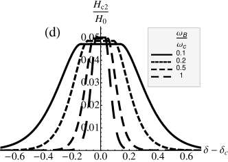
Figure 11: The upper critical field $H_{c2}$ over $H_{0}\equiv\phi_{0}a_{c}^{-2}/(2\pi)$ as a function of the distance away from criticality (a) for various scaling exponent $\alpha_{p}$’s with $\lambda=0.06,\omega_{B}/\omega_{c}=0.1,\nu=1/2,z=3$, (b) for various glue strength $\lambda$’s with $\omega_{B}/\omega_{c}=0.1,\nu=1/2,z=3,\alpha_{p}=5/6$, (c) for various $\nu$’s with $\lambda=0.06,\omega_{B}/\omega_{c}=0.1,\alpha_{p}=5/6,z=3$, (d) for various retardation ranges with $\lambda=0.06,\nu=1/2,z=3,\alpha_{p}=5/6$.

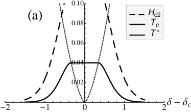
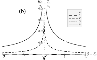
Figure 12: (a)Illustration of the different behavior of $T_{c}$ and upper critical field $H_{c2}$ as the quantum critical point is approached. $H_{c2}$ increases much faster than $T_{c}$. Thus for a small $T_{c}$ one can still have a large upper critical field. Here we plotted using the parameters $\lambda=0.05,\omega_{B}/\omega_{c}=0.1,\nu=1/2,z=3,\eta=-1$. (b) The difference $H_{c2}/H_{0}-T_{c}/\omega_{c}$ as a function of the distance away from the critical point for different dynamical exponent $z$’s. Here $H_{0}\equiv\phi_{0}a_{c}^{-2}/(2\pi)$, $\lambda=0.06,\omega_{B}/\omega_{c}=0.1,\nu z=0.5,\alpha_{p}=0.4$. For $z=2$, the difference is 0. For $z=3,4$, the difference is positive and increases rapidly when approaching the critical point. For the case with $z=1$, the difference is negative.

Modeling the variation of $H_{c2}$ in the vicinity of the QPT as in the previous paragraph, where the critical modes govern the short distance and BCS type behavior is recovered at large distance, while converting the cross-over temperature to a length scale $r^{*}$, by $T^{*}/\omega_{c}=(r^{*}/a_{c})^{-z}$, we find that $H_{c2}$ is determined by the equation,

$$\frac{1}{{\Omega^{d-1}g}}=\int_{r_{0}}^{r^{*}}\frac{{\cal C}_{h}}{r^{d-2+\eta_{p}}}r^{d-1}dr+\int^{l}_{r^{*}}\frac{{\cal C}^{\prime}_{h}}{r^{d}}r^{d-1}dr,$$ (43)

with the matching condition ${\cal C}_{h}=(r^{*})^{-2+\eta_{p}}{\cal C}^{\prime}_{h}$. We find that one just has to replace the first two dynamic exponent $z$’s in Eq. (35) by $2$ while an extra factor of 2 has to be added to the second term in the exponent,

$$H_{c2}=\frac{\phi_{0}a_{c}^{-2}}{2\pi}x^{2\nu}\left(\frac{2\omega_{B}}{\omega_{c}}\right)^{2/z}\exp\left[\frac{2}{2-\eta_{p}}\left(1-x^{\nu(2-\eta_{p})}-(\frac{2\omega_{B}}{\omega_{c}})^{\alpha_{p}}\frac{x^{\nu(2-\eta_{p})}}{\tilde{\lambda}}\right)\right].$$ (44)

In the region where only the Fermi-liquid quasiparticles contribute, the upper critical field has still an exponential form,

$$H_{c2}=\frac{\phi_{0}a_{c}^{-2}}{2\pi}\left(\frac{2\omega_{B}}{\omega_{c}}\right)^{2/z}\exp\left[-2(\frac{2\omega_{B}}{\omega_{c}})^{\frac{2-\eta_{p}}{z}}\frac{x^{\nu(2-\eta_{p})}}{(2-\eta)\tilde{\lambda}}\right].$$ (45)

The dependence of $H_{c2}$ on various parameters is shown in Fig. 11, and one infers that $H_{c2}$ behaves in ways very similar $T_{c}$ (Fig. 10). The interesting part is illustrated in Fig.(12b) where we plot $H_{c2}/H_{0}-T_{c}/\omega_{c}$ as a function of the distance away from the critical point for different dynamical exponent $z$’s, keeping all other quantities fixed, defining $H_{0}\equiv\phi_{0}a_{c}^{-2}/(2\pi)$. One infers that when $z>2$, $H_{c2}/H_{0}-T_{c}/\omega_{c}$ increases rapidly when approaching the critical point.

Using a ’ferromagnetic’ dynamical exponent $z=3$ and a Grüneisen exponent $1/\nu z=2/3$ inspired on recent experiments Kuchler et al. (2003); Tokiwa et al. (2009) as well as theoretical considerations Hertz (1976); Millis (1993); Moriya and Takimoto (1995); Si et al. (2001); Pepin (2005); Senthil (2008) we obtain the results in Fig. (12a). Compared to $T_{c}$, $H_{c2}$ peaks much more strongly towards the QCP. This is in remarkable qualitative agreement with the recent results by Levy et al. on the behavior of the orbital limiting field in ${\rm URhGe}$ exhibiting a ferromagnetic QCPLevy et al. (2007), where the highest $T_{c}$ is about 0.5 K Lévy et al. (2005), while the upper critical field exceeds 28 T. It has also been observed in noncentrosymmetric heavy fermion superconductors ${\rm CeRhSi}_{3}$ Kimura et al. (2005); Muro et al. (2007) and ${\rm CeIrSi}_{3}$ Sugitani et al. (2006); Okuda et al. (2007), where the Pauli limiting effect is suppressed due to lack of inversion center of the crystal structures and the orbital limiting effect plays the main role of pair breaking. Near the quantum critical points, $H_{c2}$ can be as high as about 30 K, although the zero field $T_{c}$ is of order 1K Kimura et al. (2007); Settai et al. (2008). This class of experiments can be understood in our framework as resulting from the change of the scaling relation between $H_{c2}$ and $T_{c}$. (See also Tada et al. (2008) for a tentative explanation from the customary Hertz-Millis-Moriya perspective.)

VII Conclusions

Perhaps the real significance of the above arguments is no more than to supply a cartoon, a metaphor to train the minds on thinking about pairing instabilities in non Fermi-liquids. This scaling theory has the merit of being mathematically controlled, given the starting assumptions of the ’retarded glue’ and conformal invariance. The Migdal parameter plays an identical role as in conventional BCS theory to yield a full control over the glue-fermion system dynamics, while we trade in Fermi-liquid principle for the even greater powers of scale invariance. The outcomes are gap and Tc equations where the standard BCS/Eliasberg equations show up as quite special cases associated with the marginality of the pair operators of the Fermi gas. The difficulty is of course to demonstrate that these starting assumptions have dealings with either nature itself and/or microscopic theories of electron systems where they should show up as emergent phenomena at low energy. However, the same objections apply to much of the current thinking regarding superconducting instabilities at quantum critical points with their implicit referral to a hidden Fermi gas. In such considerations there is an automatism to assume that eventually the superconductivity has to be governed by Eliashberg type equations. At the least, the present analysis indicates that such equations are not divine as long as the Fermi-liquid is not detected directly. Stronger, in line with the present analysis one might wish to conclude that superconducting instabilities will be generically more muscular in any non-Fermi-liquid. The Fermi-liquid is singular in the regard that its degrees of freedom are stored in the Fermi-sea, and this basic physics is responsible for the exponential smallness of the gap in terms of the coupling constant. This exponential smallness should be alien to any non Fermi-liquid.

How about experiment? Scaling theories have a special status in physics because they guide the analysis of experimental data in terms of a minimal a-priori knowledge other than scale invariance. The present theory has potentially the capacity to produce high quality empirical tests in the form of scaling collapses. However, there is a great inconvenience: one has to be able to vary the glue coupling strength, retardation parameters and so forth, at will to test the scaling structure of the equations. These are parameters associated with the materials themselves, and one runs into the standard difficulty that it is impossible to vary these in a controlled manner. What remain are the rather indirect strategies discussed in the last two sections: find out whether hidden relations exist between the detailed shape of the superconducting and the crossover lines; are there scaling relations between $H_{c2}$ and $T_{c}$ as discussed in the last section? We look forward to experimental groups taking up this challenge.

There appears to be one way to interrogate our starting assumptions in a very direct way by experiment. Inspired by theoretical work by Ferrell Ferrell (1969) and Scalapino Scalapino (1970), Anderson and Goldman showed quite some time ago Anderson and Goldman (1970) that the dynamical pair susceptibility can be measured directly using the AC Josephon effect – see also Takayama (1971); Yoshihiro and Kajimura (1970), for a recent review see ref.Goldman (2006). It would be interesting to find out whether this technique can be improved to measure the pair susceptibility over the large frequency range, ’high’ temperatures and high resolution to find out whether it has the conformal shape. It appears to us that the quantum critical heavy fermion superconductors offer in this regard better opportunities than e.g. the cuprates given their intrinsically much smaller energy scales.

In conclusion, exploiting the motives of retardation and conformal invariance we have devised a phenomenological scaling theory for superconductivity that generalizes the usual BCS theory to non Fermi-liquid quantum critical metals. The most important message of this simple construction is that it demonstrates the limitations of the usual Fermi-liquid BCS theory. The exponential smallness of the gap in the coupling is just reflecting the ’asymptotic freedom’ of the Fermi-liquid, and this is of course a very special case within the landscape of scaling behaviors. Considering the case that the pair operator is relevant, we find instead an ’algebraic’ gap equation revealing that at weak couplings and strong retardation the rules change drastically: as long as the electronic UV cut-off and the glue energy are large, one can expect high $T_{c}$’s already for quite weak electron-phonon like couplings. If our hypothesis turns out to be correct, this solves the problem of superconductivity at a high temperature although it remains to be explained why quantum critical normal states can form with the required properties. It is however not straightforward to device a critical test for our hypothesis. The problem is the usual one that pair susceptibilities, $\lambda$’s or $\alpha^{2}F$’s, and so forth cannot be measured directly and one has to rely on imprecise modelling. However, it appears to us that ’quantum critical BCS superconductivity’ works so differently from the Fermi-liquid case that it eventually should be possible to nail it down in the laboratory. We hope that the sketches in the above will form a source of inspiration for future work.

Acknowledgements We acknowledge useful discussions with M. Sigrist, D. van der Marel, A.V. Balatsky, B. J. Overbosch, D.J. Scalapino, K. Schalm and S. Sachdev. This work is supported by the Nederlandse Organisatie voor Wetenschappelijk Onderzoek (NWO) via a Spinoza grant.

References

- Mathur et al. (1998) N. D. Mathur et al., Nature 394, 39 (1998).
- Zaanen (2008) J. Zaanen, Science 319, 5867 (2008), and references therein.
- Stewart (2006) G. R. Stewart, Rev. Mod. Phys. 73, 797 (2006).
- von Löhneisen et al. (2007) H. von Löhneisen, A. Rosch, M. Vojta, and P. Wölfle, Rev. Mod. Phys. 79, 1015 (2007).
- Coleman et al. (2001) P. Coleman, C. Pépin, Q. Si, and R. Ramazashvili, J. Phys: Cond. Mat. 13, 723 (2001).
- Coleman and Schofield (2005) P. Coleman and A. J. Schofield, Nature 433, 226 (2005).
- Gegenwart et al. (2008) P. Gegenwart, Q. Si, and F. Steglich, Nature Physics 4, 186 (2008).
- Paschen et al. (2004) S. Paschen et al., Nature 432, 881 (2004).
- Si et al. (2001) Q. Si, S. Rabello, K. Ingersent, and J. L. Smith, Nature 413, 804 (2001).
- van der Marel et al. (2003) D. van der Marel et al., Nature 425, 271 (2003).
- Cooper et al. (2009) R. A. Cooper et al., Science 323, 603 (2009).
- Bud’ko et al. (2009) S. L. Bud’ko, N. Ni, and P. C. Canfield, Phys. Rev. B 79, 220516 (2009).
- Zaanen (2009) J. Zaanen (2009), eprint arXiv:0908.0033[cond-mat.supr-con].
- Varma et al. (1989) C. M. Varma, P. B. Littlewood, S. Schmitt-Rink, E. Abrahams, and A. E. Ruckenstein, Phys. Rev. Lett. 63, 1996 (1989).
- Monthoux et al. (2007) P. Monthoux, D. Pines, and G. G. Lonzarich, Nature 450, 1177 (2007).
- Chubukov and Sachdev (1993) A. V. Chubukov and S. Sachdev, Phys. Rev. Lett. 71, 169 (1993).
- Varma et al. (2002) C. M. Varma, Z. Nussinov, and W. van Saarloos, Phys. Rep. 361, 267 (2002).
- Bonesteel et al. (1996) N. E. Bonesteel, I. A. McDonald, and C. Nayak, Phys. Rev. Lett. 77, 3009 (1996).
- Galitski and Sachdev (2009) V. Galitski and S. Sachdev, Phys. Rev. B 79, 134512 (2009).
- Chubukov and Schmalian (2005) A. V. Chubukov and J. Schmalian, Phys. Rev. B 72, 174520 (2005).
- Chubukov and Tsvelik (2007) A. V. Chubukov and A. M. Tsvelik, Phys. Rev. B 76, 100509 (2007).
- Abanov et al. (2001a) A. Abanov, A. V. Chubukov, and A. M. Finkel’stein, Euro. Phys. Lett. 54, 488 (2001a).
- Abanov et al. (2001b) A. Abanov, A. V. Chubukov, and J. Schmalian, Euro. Phys. Lett. 55, 369 (2001b).
- Chubukov et al. (2003) A. V. Chubukov, A. M. Finkel’stein, R. Haslinger, and D. K. Morr, Phys. Rev. Lett. 90, 077002 (2003).
- Krotkov and Chubukov (2006a) P. Krotkov and A. V. Chubukov, Phys. Rev. Lett. 96, 107002 (2006a).
- Krotkov and Chubukov (2006b) P. Krotkov and A. V. Chubukov, Phys. Rev. B 74, 014509 (2006b).
- Abanov et al. (2008) A. Abanov, A. V. Chubukov, and M. R. Norman, Phys. Rev. B 78, 220507 (2008).
- Khveshchenko and Shively (2006) D. V. Khveshchenko and W. F. Shively, Phys. Rev. B 73, 115104 (2006).
- Moon and Sachdev (2009) E. G. Moon and S. Sachdev, Phys. Rev. B 80, 035117 (2009).
- Fisk and Pines (1998) Z. Fisk and D. Pines, Nature 394, 22 (1998).
- Mazin and Singh (1997) I. I. Mazin and D. J. Singh, Phys. Rev. Lett. 79, 733 (1997).
- Monthoux and Lonzarich (1999) P. Monthoux and G. G. Lonzarich, Phys. Rev. B 59, 14598 (1999).
- Fay and Appel (1980) D. Fay and J. Appel, Phys. Rev. B 22, 3173 (1980).
- Millis et al. (1988) A. Millis, S. Sachdev, and C. M. Varma, Phys. Rev. B 37, 4975 (1988).
- Franz and Millis (1998) M. Franz and A. J. Millis, Phys. Rev. B 58, 14572 (1998).
- Roussev and Millis (2001) R. Roussev and A. J. Millis, Phys. Rev. B 63, 140504 (2001).
- Blagoev et al. (1999) K. B. Blagoev, J. R. Engelbrecht, and K. S. Bedell, Phys. Rev. Lett. 82, 133 (1999).
- Wang et al. (2001) Z. Wang, W. Mao, and K. Bedell, Phys. Rev. Lett. 87, 257001 (2001).
- Allen and Dynes (1975) P. B. Allen and R. C. Dynes, Phys. Rev. B 12, 905 (1975).
- Marsiglio and Carbotte (1986) F. Marsiglio and J. P. Carbotte, Phys. Rev. B 33, 6141 (1986).
- Carbotte (1990) J. P. Carbotte, Rev. Mod. Phys. 62, 1027 (1990).
- Scalapino et al. (1986) D. J. Scalapino, E. Loh, and J. E. Hirsch, Phys. Rev. B 34, 8190 (1986).
- Bulaevskii and Zyskin (1990) L. N. Bulaevskii and M. V. Zyskin, Phys. Rev. B 42, 10230 (1990).
- Kirkpatrick et al. (2001) T. R. Kirkpatrick, D. Belitz, T. Vojta, and R. Narayanan, Phys. Rev. Lett. 87, 127003 (2001).
- Sandeman et al. (2003) K. G. Sandeman, G. G. Lonzarich, and A. J. Schofield, Phys. Rev. Lett. 90, 167005 (2003).
- Strack et al. (2009) P. Strack, S. Takei, and W. Metzner (2009), eprint arXiv:0905.3894v1 [cond-mat.str-el].
- Son (1999) D. T. Son, Phys. Rev. D 59, 094019 (1999).
- Dolgov and Maksimov (1982) O. V. Dolgov and E. G. Maksimov, Sov. Phys. Usp. 25, 688 (1982).
- Dolgov et al. (2008) O. Dolgov, I. Mazin, A. Golubov, S. Savrasov, and E. Maksimov, J. Phys: Cond. Mat. 20, 434226 (2008).
- Combescot (1997) R. Combescot, Euro. Phys. Lett. 43, 701 (1997).
- Hertz (1976) J. A. Hertz, Phys. Rev. B 14, 1165 (1976).
- Troyer and Wiese (2005) M. Troyer and U. Wiese, Phys. Rev. Lett. 94, 17201 (2005).
- Krüger and Zaanen (2008) F. Krüger and J. Zaanen, Phys. Rev. B 78, 035104 (2008).
- Cubrovic et al. (2009) M. Cubrovic, J. Zaanen, and K. Schalm (2009), eprint arXiv:0904.1993[hep-th].
- Senthil (2008) T. Senthil, Phys. Rev. B 78, 035103 (2008).
- Liu et al. (2009) H. Liu, J. McGreevy, and D. Vegh (2009), eprint arXiv:0903.2477[hep-th].
- Faulkner et al. (2009) T. Faulkner, H. Liu, J. McGreevy, and D. Vegh (2009), eprint arXiv:0907.2694[hep-th].
- Schrieffer (1971) J. R. Schrieffer, Theory Of Superconductivity (Perseus Publishing, 1971).
- Levy et al. (2007) F. Levy, I. Sheikin, and A. Huxley, Nature Physics 3, 460 (2007).
- Balatsky (1993) A. Balatsky, Philos. Mag. Lett. 68, 251 (1993).
- Sudbo (1995) A. Sudbo, Phys. Rev. Lett. 74, 2575 (1995).
- Yin and Chakravarty (1996) L. Yin and S. Chakravarty, Int. J. Mod. Phys. B 10, 805 (1996).
- Muck and Viswanathan (1998) W. Muck and K. S. Viswanathan, Phys. Rev. D 58, 041901 (1998).
- Freedman et al. (1999) D. Freedman, S. Mathur, A. Matusis, and L. Rastelli, Phys. Lett. B 452, 61 (1999).
- D’Hoker and Freedman (1998a) E. D’Hoker and D. Freedman, Nucl. Phys. B 544, 612 (1998a).
- Liu (1998) H. Liu, Phys. Rev. D 60, 106005 (1998).
- D’Hoker and Freedman (1998b) E. D’Hoker and D. Z. Freedman, Nucl. Phys. B 550, 261 (1998b).
- D’Hoker et al. (1999) E. D’Hoker, D. Z. Freedman, S. D. Mathur, A. Matusis, and L. Rastelli, Nucl. Phys. B 562, 353 (1999).
- Chalmers and Schalm (1998) G. Chalmers and K. Schalm, Nucl. Phys. B 554, 215 (1998).
- Chalmers and Schalm (1999) G. Chalmers and K. Schalm, Phys. Rev. D 61, 046001 (1999).
- Allen (1980) P. B. Allen, in Modern Trends in the Theory of Condensed Matter, edited by A. Pekalski and J. Przystawa (Springer-Verlag, 1980).
- Sachdev (1999) S. Sachdev, Quantum Phase Transitions (Cambridge University Press, New York, 1999).
- Uchoa and Neto (2007) B. Uchoa and A. H. C. Neto, Phys. Rev. Lett. 98, 146801 (2007).
- Kopnin and Sonin (2008) N. B. Kopnin and E. B. Sonin, Phys. Rev. Lett. 100, 246808 (2008).
- Neto (2001) A. H. C. Neto, Phys. Rev. Lett. 86, 4382 (2001).
- Uchoa et al. (2005) B. Uchoa, G. G. Cabrera, and A. H. C. Neto, Phys. Rev. B 71, 184509 (2005).
- Lee et al. (2006) J. Lee et al., Nature 442, 546 (2006).
- Damascelli et al. (2003) A. Damascelli, Z. Hussain, and Z. X. Shen, Rev. Mod. Phys. 75, 473 (2003).
- (79) E. van Heumen et al., eprint arXiv:0904.1223[cond-mat.supr-con].
- Dzyaloshinskii (1996) I. E. Dzyaloshinskii, J. Phys. I France 6, 119 (1996).
- Irkhin et al. (2001) V. Y. Irkhin, A. A. Katanin, and M. I. Katsnelson, Phys. Rev. B 64, 165107 (2001).
- Irkhin et al. (2002) V. Y. Irkhin, A. A. Katanin, and M. I. Katsnelson, Phys. Rev. Lett. 89, 076401 (2002).
- Rubtsov et al. (2009) A. N. Rubtsov, M. I. Katsnelson, A. I. Lichtenstein, and A. Georges, Phys. Rev. B 79, 045133 (2009).
- Millis (1993) A. J. Millis, Phys. Rev. B 48, 7183 (1993).
- Moriya and Takimoto (1995) T. Moriya and T. Takimoto, J. Phys. Soc. Jpn. 64, 960 (1995).
- Pepin (2005) C. Pepin, Phys. Rev. Lett. 94, 066402 (2005).
- Custers et al. (2003) J. Custers et al., Nature 424, 524 (2003).
- Zhu et al. (2003) L. Zhu, M. Garst, A. Rosch, and Q. Si, Phys. Rev. Lett. 91, 066404 (2003).
- Zaanen and Hosseinkhani (2004) J. Zaanen and B. Hosseinkhani, Phys. Rev. B 70, 060509 (2004).
- Rajagopal and Vasudevan (1966) A. K. Rajagopal and R. Vasudevan, Phys. Lett. 23, 539 (1966).
- Abrikosov et al. (1963) A. A. Abrikosov, L. P. Gorkov, and I. E. Dzayloshinskii, Methods of Quantum Field Theory in Statistical Physics (Dover, New York, 1963).
- Dias and Wheatley (1994) R. G. Dias and J. M. Wheatley, Phys. Rev. B 50, 13887 (1994).
- Schofield (1995) A. J. Schofield, Phys. Rev. B 51, 11733 (1995).
- Helfand and Werthamer (1966) E. Helfand and N. R. Werthamer, Phys. Rev. B 147, 288 (1966).
- Kuchler et al. (2003) R. Kuchler et al., Phys. Rev. Lett. 91, 066405 (2003).
- Tokiwa et al. (2009) Y. Tokiwa et al., Phys. Rev. Lett. 102, 066401 (2009).
- Lévy et al. (2005) F. Lévy, I. Sheikin, B. Grenier, and A. D. Huxley, Science 309, 1343 (2005).
- Kimura et al. (2005) N. Kimura, K. Ito, K. Saitoh, Y. Umeda, H. Aoki, and T. Terashima, Phys. Rev. Lett. 95, 247004 (2005).
- Muro et al. (2007) Muro et al., J. Phys. Soc. Jpn. 76, 033706 (2007).
- Sugitani et al. (2006) I. Sugitani et al., J. Phys. Soc. Jpn. 75, 043703 (2006).
- Okuda et al. (2007) Y. Okuda et al., J. Phys. Soc. Jpn. 76, 044708 (2007).
- Kimura et al. (2007) N. Kimura, K. Ito, H. Aoki, S. Uji, and T. Terashima, Phys. Rev. Lett. 98, 197001 (2007).
- Settai et al. (2008) R. Settai, Y. Miyauchi, T. Takeuchi, F. Lévy, I. Siieikin, and Y. Onuki, J. Phys. Soc. Jpn. 77, 073705 (2008).
- Tada et al. (2008) Y. Tada, N. Kawakami, and S. Fujimoto, Phys. Rev. Lett. 101, 267006 (2008).
- Ferrell (1969) R. A. Ferrell, J. Low Temp. Phys. 1, 423 (1969).
- Scalapino (1970) D. J. Scalapino, Phys. Rev. Lett. 24, 1052 (1970).
- Anderson and Goldman (1970) J. T. Anderson and A. M. Goldman, Phys. Rev. Lett. 25, 743 (1970).
- Takayama (1971) H. Takayama, Prog. Theor. Phys. (Japan) 46, 1 (1971).
- Yoshihiro and Kajimura (1970) K. Yoshihiro and K. Kajimura, Phys. Lett. 32A, 71 (1970).
- Goldman (2006) A. M. Goldman, Journal of Superconductivity and Novel Magnetism 19, 317 (2006).