Matrix Graph Grammars as a Model of Computation

Abstract

Matrix Graph Grammars (MGG) is a novel approach to the study of graph dynamics ([16]). In the present contribution we look at MGG as a formal grammar and as a model of computation, which is a necessary step in the more ambitious program of tackling complexity theory through MGG. We also study its relation with other well-known models such as Turing machines (TM) and Boolean circuits (BC) as well as non-determinism. As a side effect, all techniques available for MGG can be applied to TMs and BCs.

Keywords: Matrix Graph Grammars, Graph Dynamics, Graph Transformation, Graph Rewriting, Model of Computation.

1 Introduction

Graph transformation [4, 20] is becoming increasingly popular in order to describe system behavior due to its graphical, declarative and formal nature. It is central to many application areas, such as visual languages, visual simulation, picture processing and model transformation (see [4] and [20] Vol.2 for some applications). Also, graph rewriting techniques have proved useful in describing Domain Specific Languages and in language-oriented programming (see [8]).

Matrix Graph Grammars (MGG) is a purely algebraic approach to graph rewriting (graph dynamics) that has successfully solved or extended problems and results such as sequentialization, explicit parallelism, applicability, congruence characterization, initial state calculation (initial digraphs), constraints (application conditions) and reachability. See for example [12, 13, 14, 15, 18, 19] or the more comprehensive introduction [16].

It seems natural to study MGG as a model of computation that would describe the state of some system by means of graphs. To the very best of the author’s knowledge, there has been no attempt in this direction until now, despite the agreed interest of the topic (see e.g. [9, 10]). Even more so, there seems to be no graph rewriting literature on non-determinism or, more generally, on complexity.

There are two main handicaps that may partially explain the lack of theoretical results. First, graph rewriting systems (MGG in particular) would make use of the functional problem known as subgraph matching. Its associated decision problem (subgraph isomorphism) has been proved to be NP-complete ([6]). Even worse, subgraph matching would be used in every single step of the computation. Second, there are two apparently hard-to-avoid sources of non-determinism: what production rule to apply and where to apply it.

The author’s main motivation for the development of MGG is the study of complexity theory – complexity classes P and NP in particular – which has led the research in MGG up to now. The present contribution is a necessary step in this program.

Due to their current theoretical and practical relevance, we have decided to study Turing machines (TM) and Boolean Circuits (BC) and compare them to MGG. As a side effect, all techniques developed for MGG become available to study TMs and BCs. Currently we are capable to (partially) answer the following questions within MGG:

1. Coherence: are the actions specified by the productions (inside a sequence) compatible with each other?

2. Initial state: calculate an initial configuration (initial grammar state) such that some given sequence can be applied.

3. Congruence: do a sequence and a permutation of it have a common initial state?

4. Sequential independence: is it possible to advance/delay some production a finite number of positions inside a given sequence?

5. Reachability: for a given grammar and initial and final states, find a sequence that transforms the initial state into the final state.

Paper Organization. Section 2 is an overview of the very basics of MGG and briefly explains some of the analysis techniques developed so far. Section 3 characterizes relabeling in MGG. Section 4 and 5 study MGG as a formal grammar and as a model of computation, respectively, touching on some possible submodels and supermodels of computation that can be defined from MGG. Determinism is addressed in Secs. 6 and 7, in which we move from Boolean algebra to an algebra of matrices. In Secs. 8 and 9 MGG models Turing machines and Boolean Circuits, respectively. Section 10 closes this paper with a short summary and some proposals for future research.

Notation. The matrix whose entries are all zero will be represented with a bolded zero, 0. Similarly, the matrix in which every single element is a one will be represented with a bolded one, 1.

2 Matrix Graph Grammars: Basics

In this section we give a brief overview of some of the basics of Matrix Graph Grammars (MGG) with examples as intuitive as possible. For a detailed account and accessible presentation the reader is referred to [16].
 
 Simple Digraphs. We work with simple digraphs, which we represent as $(M,V)$ where $M$ is a Boolean matrix for edges (the graph adjacency matrix) and $V$ a Boolean vector for vertices or nodes. Note that we explicitly represent the nodes of the graph with a vector. This is necessary because it is possible within MGG to add and delete nodes.

The existing nodes are marked with a $1$ in the corresponding position of the vector. Figure 1(a) shows a graph representing a production system made of a machine (controlled by an operator) which consumes and produces pieces through conveyors. Generators create pieces in conveyors. Self loops in operators and machines indicate that they are busy.

Figure 1: Simple Digraph Example (left). Matrix Representation with Labels (right)

Note that the matrix and the vector in the figure are the smallest ones able to represent the graph. Adding $0$-elements to the vector (and accordingly $0$-rows and columns to the matrix) would result in equivalent graphs. Next definition formulates the representation of simple digraphs.

Definition 1 (Simple Digraph Representation)

A simple digraph $G$ is represented by $G=(M,V)$ where $M$ is the graph adjacency matrix and $V$ is the Boolean vector of its nodes.

Compatibility. Well-formedness of graphs (i.e. absence of dangling edges) can be checked by verifying the identity $\left\|\left(M\vee M^{t}\right)\odot\overline{V}\right\|_{1}=0$, where $\odot$ is the Boolean matrix product (like the regular matrix product, but with and and or instead of multiplication and addition), $M^{t}$ is the transpose of the matrix $M$, $\overline{V}$ is the negation of the nodes vector $V$, and $\|\cdot\|_{1}$ is an operation (a norm, actually) that results in the or of all the components of the vector. This property is called compatibility in [12]. Note that $M\odot\overline{V}$ results in a vector that contains a $1$ in position $i$ when there is an outgoing edge from node $i$ to a non-existing node. A similar expression with the transpose of $M$ is used to check for incoming edges. A simple digraph $G=(M,V)$ is compatible if and only if

$$\left\|\left(M\vee M^{t}\right)\odot\overline{V}\right\|_{1}=0.$$ (1)

Compatibility of productions guarantees that the image of a simple digraph is a simple digraph again. It is useful to check closedness of the space (simple digraphs) under the specified operations (grammar rules).
 
 Labeling. A label (also known as a type) is assigned to each node in $G=(M,V)$ by a function from the set of nodes $V$ to a set of labels $\mathcal{T}$, $\lambda:V\rightarrow\mathcal{T}$. In Fig. 1 labels are represented as an extra column in the matrices, the numbers before the colon distinguish elements of the same type.

There are several equivalent possibilities to label edges. We may use the types of their source and target nodes. Another possibility is to choose the set of edges $E(G)$ as domain for $\lambda$ (see Def. 2) instead of $V$. Notice that this would define $\lambda$ for every element in the adjacency matrix. Yet another possibility is to define labels just on nodes and split one edge $N_{1}N_{2}$ (the one joining node $N_{1}$ to node $N_{2}$) into two edges, the first starting in node $N_{1}$ and ending in a “labeling node” and the second starting in this same “labeling node” and ending in $N_{2}$.

Definition 2 (Labeled Simple Digraph)

A labeled simple digraph $G_{\lambda}=(G,\lambda)=((M,V),\lambda)$ over a set of labels $\mathcal{T}$ is made of a simple digraph $G$ plus a function $\lambda:V\rightarrow\mathcal{T}$ whose domain is the set of nodes of $G$.

By abuse of notation, the subscript $\lambda$ will normally be omitted. Next we define the notion of partial morphism between labeled simple digraphs.

Definition 3 (Labeled Simple Digraph Morphism)

Given two simple digraphs $G_{i}=((M_{i},V_{i}),\lambda_{i}:V_{i}\rightarrow\mathcal{T})$ for $i=\{1,2\}$, a morphism $f=(f^{V},f^{E}):G_{1}\rightarrow G_{2}$ is made of two partial injective functions $f^{V}:V_{1}\rightarrow V_{2}$, $f^{E}:M_{1}\rightarrow M_{2}$ between the set of nodes and edges, such that:

1. $\forall v\in Dom(f^{V}),\>\lambda_{1}(v)=\lambda_{2}\left(f^{V}(v)\right)$

2. $\forall(n,m)\in Dom(f^{E}),\>f^{E}(n,m)=\left(f^{V}(n),f^{V}(m)\right)$,

where $Dom(f)$ is the domain of the partial function $f$, $E$ stands for edges and $V$ for vertices.

Productions. A production, $p:L\rightarrow R$ is a morphism of labeled simple digraphs. Using a static formulation, a rule is represented by two labeled simple digraphs that encode the left and right hand sides (LHS and RHS, respectively). The matrices and vectors of these graphs are arranged so that the elements identified by morphism $p$ match (this is called completion, see below).

Definition 4 (Static Formulation of Productions)

A production $p:L\rightarrow R$ is statically represented as

$$p=(L,R)=\left((L^{E},L^{V},\lambda_{L}),(R^{E},R^{V},\lambda_{R})\right).$$ (2)

A production adds and deletes nodes and edges, therefore using a dynamic formulation, we can encode the rule’s pre-condition (its LHS) together with matrices and vectors representing the addition and deletion of edges and nodes. We call such matrices and vectors $e$ for “erase” and $r$ for “restock”.

Definition 5 (Dynamic Formulation of Productions)

A production $p:L\rightarrow R$ is dynamically represented as

$$p=(L,e,r)=\left(\left(L^{E},L^{V},\lambda_{L}\right),\left(e^{E},e^{V},\lambda_{e}\right),\left(r^{E},r^{V},\lambda_{r}\right)\right),$$ (3)

where $e^{E}$ and $e^{V}$ are the deletion Boolean matrix and vector (respectively), $r^{E}$ and $r^{V}$ are the addition Boolean matrix and vector (respectively). They have a $1$ in the position where the element is to be deleted (for $e$) or added (for $r$).

The output of rule $p$ – where the and symbol $\wedge$ is omitted to simplify formulae – is calculated by the Boolean formula

$$R=p(L)=r\vee\overline{e}L,$$ (4)

which applies to both, edges and nodes.

Example.$\square$Figure 2 shows a rule and its associated matrices. The rule models the consumption of a piece by a machine. Compatibility of the resulting graph must be ensured, thus the rule cannot be applied if the machine is already busy, as it would end up with two self loops, which is not allowed in a simple digraph. This restriction of simple digraphs can be useful in this kind of situations, and acts like a built-in negative application condition (refer to [16], Chaps. 8 and 9). Later we will see that the nihilation matrix takes care of this restriction.

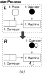
Figure 2: (a) Rule Example. (b) Static Formulation. (c) Dynamic Formulation.

Completion. In order to operate graphs of different sizes, an operation called completion adds extra rows and columns with zeros (to matrices and vectors) and rearranges rows and columns so that the identified edges and nodes of the two graphs match. For example, in Fig. 2, if $L^{E}$ and $R^{E}$ need to be operated, completion adds a fourth 0-row and fourth 0-column to $R^{E}$.

Otherwise stated, whenever we have to operate graphs $G_{1}$ and $G_{2}$, an implicit morphism $f:G_{1}\rightarrow G_{2}$ has to be established. This morphism is completion, which rearranges the matrices and the vectors of both graphs so that the elements match. In the examples, we omit such operation, and assume that matrices are completed when necessary.
 
 Nihilation Matrix. In order to consider the elements in the host graph that disable a rule application, we extend the notation for rules with a new graph $K$. Its associated matrix specifies the two kinds of forbidden edges: those incident to nodes which are going to be erased and any edge added by the rule (which cannot be added twice, since we are dealing with simple digraphs). Notice however that $K$ considers only potential dangling edges with source and target in the nodes belonging to $L^{V}$.

Definition 6 (Nihilation Matrix)

Given the production $p=(L,e,r)$, its nihilation matrix $K^{E}$ contains non-zero elements in positions corresponding to newly added edges, and to non-deleted edges adjacent to deleted nodes.

We extend the rule formulation with this nihilation matrix. The concept of production remains unaltered because we are just making explicit some implicit information. Matrices are derived in the following order: $\left(L,R\right)\mapsto\left(e,r\right)\mapsto K$. Thus, a rule is statically determined by its LHS and RHS $p=\left(L,R\right)$, from which it is possible to give a dynamic definition $p=\left(L,e,r\right)$, with $e=L\overline{R}$ and $r=R\overline{L}$, to end up with a full specification including its environmental behavior $p=\left(L,K,e,r\right)$. No extra effort is needed from the grammar designer because $K$ can be automatically calculated as the image by the rule $p$ of a certain matrix (see below).

Notice that the nihilation matrix $K$ for a production $p$ has an associated simple digraph whose nodes coincide with those of $L$ as well as its labels.

Definition 7 (Dynamic Reformulation of Production)

A production $p:L\rightarrow R$ is dynamically represented as

$$p =(L,K,e,r,\lambda)=$$

$$=\left(\left(L^{E},L^{V},\lambda_{L}\right),\left(K^{E},K^{V},\lambda_{K}\right),\left(e^{E},e^{V},\lambda_{e}\right),\left(r^{E},r^{V},\lambda_{r}\right)\right),$$ (5)

where $L$ is the LHS, $K$ is the labeled simple digraph associated to the nihilation matrix, $e$ is the deletion matrix and $r$ is the addition matrix.

The nihilation matrix $K^{E}$ of a given production $p$ is given by

$$K^{E}=p\left(\overline{D}\right)\quad\mathrm{with}\quad D=\overline{e^{V}}\otimes\overline{e^{V}}^{t},$$ (6)

where $\otimes$ denotes the tensor (or Kronecker) product, which sums up the covariant and contravariant parts and multiplies every element of the first vector by the whole second vector. See [19] for a proof. Notice that matrix $\overline{D}$ specifies potential dangling edges incident to nodes in $p$’s LHS:

$$\overline{D}=d^{i}_{\!j}=\left\{\begin{array}[]{ll}1&\qquad if\;(e^{V})^{i}=1\;or\;(e^{V})^{j}=1.\\ 0&\qquad otherwise.\end{array}\right.$$

Example.$\square$The nihilation matrix $K^{E}$ for the example rule of Fig. 2 is calculated as follows:

$$\overline{\overline{e^{V}}\otimes\overline{\left(e^{V}\right)}^{\,t}}=\overline{\left[\begin{array}[]{c}1\\ 1\\ 1\\ 0\\ \end{array}\right]\otimes\left[\begin{array}[]{c}1\\ 1\\ 1\\ 0\\ \end{array}\right]^{t}}=\left[\begin{array}[]{cccc}0&0&0&1\\ 0&0&0&1\\ 0&0&0&1\\ 1&1&1&1\\ \end{array}\right]$$

The nihilation matrix is then given by :

$$K=r\vee\overline{e}\overline{D}=\left[\begin{array}[]{cccc}0&0&0&0\\ 0&1&0&0\\ 0&0&1&0\\ 0&0&0&0\\ \end{array}\right]\vee\overline{\left[\begin{array}[]{cccc}0&0&0&0\\ 0&0&0&0\\ 0&0&0&0\\ 1&0&0&0\\ \end{array}\right]}\left[\begin{array}[]{cccc}0&0&0&1\\ 0&0&0&1\\ 0&0&0&1\\ 1&1&1&1\\ \end{array}\right]=\left[\begin{array}[]{cccc}0&0&0&1\\ 0&1&0&1\\ 0&0&1&1\\ 0&1&1&1\\ \end{array}\right]$$

The matrix indicates any dangling edge from the deleted piece (the edge to the conveyor is not signaled as it is explicitly deleted) as well as self-loops in the machine and in the operator. $\blacksquare$

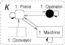
Figure 3: $K$ Graph for startProcess

The evolution of the rule LHS (i.e. how it is transformed into the RHS) is given by the production itself: $R=p(L)=r\vee\overline{e}\,L$. See equation (4). It is interesting to analyze the behavior of the nihilation matrix, which is given in the next proposition. Let $p:L\rightarrow R$ be a compatible production with nihilation graph $K$. Then, the elements that must not appear ($Q$) once the production is applied (see [19] for a proof) are given by

$$Q=p^{-1}\left(K\right)=e\vee\overline{r}\,K^{E}.$$ (7)

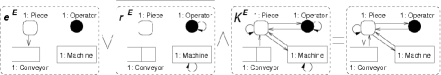
Figure 4: Evolution of the Nihilation Matrix

Example.$\square$Figure 4 shows the calculation of $startProcess^{-1}(K^{E})$ using the graph representation of the matrices in eq. (7). $\blacksquare$

The dual concept $T$ specifies the newly available edges after the application of a production due to the addition of nodes:

$$T=\left(\overline{\overline{r}\otimes\overline{r}^{t}}\right)\wedge\left(\overline{e}\otimes\overline{e}^{t}\right).$$ (8)

Refer to [18] where $T$ was introduced and studied.

Next definition introduces a functional notation for rules (already used in [13]) inspired by the Dirac or bra-ket notation [1].

Definition 8 (Functional Formulation of Production)

A production $p:L\rightarrow R$ can be depicted as $R=p(L)=\left\langle L,p\right\rangle$, splitting the static part (initial state, $L$) from the dynamics (element addition and deletion, $p$).

Using such formulation, the ket operators (i.e. those to the right of the bra-ket) can be moved to the bra (i.e. left hand side) by using their adjoints (which are usually decorated with an asterisk).
 
 Match and Derivations. Matching is the operation of identifying the LHS of a rule inside a host graph (we consider only injective matches). Given the rule $p:L\rightarrow R$ and a simple digraph $G$, any $m:L\rightarrow G$ total injective morphism is a match for $p$ in $G$. The following definition considers not only the elements that should be present in the host graph $G$ (those in $L$) but also those that should not be (those in $K$).

Definition 9 (Direct Derivation)

Given the rule $p:L\rightarrow R$ and the graph $G=(G^{E},G^{V})$ as in Fig. 5(a), $d=\left(p,m\right)$ – with $m=\left(m_{L},m^{E}_{K}\right)$ – is called a direct derivation with result $H=p^{*}\left(G\right)$ if the following conditions are fulfilled:

1. There exist $m_{L}:L\rightarrow G$ and $m^{E}_{K}:K^{E}\rightarrow\overline{G^{E}}$ total injective morphisms.

2. $m_{L}(n)=m^{E}_{N}(n)$, $\forall n\in L^{V}$.

3. The match $m_{L}$ induces a completion of $L$ in $G$. Matrices $e$ and $r$ are then completed in the same way to yield $e^{*}$ and $r^{*}$. The output is given by $H=p^{*}(G)=r^{*}\vee\overline{e^{*}}G$.

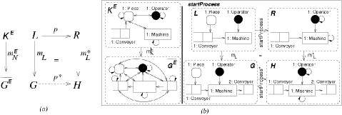
Figure 5: (a) Direct Derivation. (b) Example

Remark.$\square$The square in Fig. 5 (a) is a categorical pushout. Item 2 is needed to ensure that $L$ and $K^{E}$ are matched to the same nodes in $G$. $\blacksquare$

Example.$\square$Figure 5(b) shows the application of rule startProcess to graph $G$. We have also depicted the inclusion of $K^{E}$ in $\overline{G^{E}}$ (bidirectional arrows have been used for simplification). $\overline{G^{E}}$ is the complement (negation) of matrix $G^{E}$. $\blacksquare$

It is useful to consider the structure defined by the negation of the host graph, $\overline{G}=(\overline{G^{E}},\overline{G^{V}})$. It is made up of the graph $\overline{G^{E}}$ and the vector of nodes $\overline{G^{V}}$. Note that the negation of a graph is not a graph because in general compatibility fails, that is why the term “structure” is used.

The complement of a graph coincides with the negation of the adjacency matrix, but while negation is just the logical operation, taking the complement means that a completion has been performed in advance. That is, the complement of graph $G$ with respect to graph $A$, through a morphism $f:A\rightarrow G$ is a two-step operation: (i) complete $G$ and $A$ according to $f$, yielding $G^{\prime}$ and $A^{\prime}$; (ii) negate $G^{\prime}$. As long as no confusion arises negation and complements will not be distinguished syntactically.

Figure 6: Finding Complement and Negation of a Graph.

Examples.$\square$Suppose we have two graphs $A$ and $G$ as those depicted in Fig. 6 and that we want to check that $A$ is not in $G$. Note that $A$ is not contained in $\overline{G}$ (an operator node does not even appear) but it does appear in the negation of the completion of $G$ with respect to $A$ (graph $\overline{G}_{A}$ in the same figure).

In the context of Fig. 5(b) we see that there is an inclusion $startProcess^{-1}(K^{E})\rightarrow\overline{H}$ (i.e. the forbidden elements after applying production $startProcess$ are not in $H$). This is so because we complete $H$ with an additional piece (which was deleted from $G$). $\blacksquare$
 
 Analysis Techniques. In [12, 13, 14, 15, 16] we developed some analysis techniques, mainly to study sequences in MGG. We end this section with a short summary of these techniques with the exception of application conditions, graph constraints and explicit parallelism.

One of the goals of our previous work was to analyze rule sequences independently of a host graph. We represent a rule sequence as $s_{n}=p_{n};...;p_{1}$, where application is from right to left (i.e. $p_{1}$ is applied first). For its analysis, we complete the sequence by identifying the nodes across rules which are assumed to be mapped to the same node in the host graph. Mind the non-commutativity of this operation and its potential non-determinism.

Once the sequence is completed, our notion of sequence coherence [12] allows to know if, for the given identification, the sequence is potentially applicable (i.e. if no rule disturbs the application of those following it). The formula for coherence results in a matrix and a vector (which can be interpreted as a graph) with the problematic elements. If the sequence is coherent, both should be zero, if not, they contain the problematic elements. We shall elaborate on this in Secs. 6 and 7.

A coherent sequence is compatible if its application produces a simple digraph. That is, no dangling edges are produced in intermediate steps. This extends the notions of compatible graph and compatible production.

Given a completed sequence, the minimal initial digraph (MID) is the smallest graph that allows applying such sequence. Conversely, the negative initial digraph (NID) contains all elements that should not be present in the host graph for the sequence to be applicable. In this way, the NID is a graph that should be found in $\overline{G}$ for the sequence to be applicable (i.e. none of its edges can be found in $G$). We shall elaborate on this in Sec. 7.

We shall not touch on other concepts such as G-congruence and reachability. Notice that reachability can be thought of as an initial attempt to measure the number of elements in a sequence, a tool that might be useful to provide lower bounds. Similarly to what is done in the present contribution for Turing Machines and Boolean Circuits, Petri nets can be modeled with Matrix Graph Grammars. See [18] and [16].

3 Relabeling

Completion as introduced in Sec. 2 performs two tasks: enlarges matrices by adding rows and columns of the appropriate type and rearranges them (to get a coincidence according to the identifications across productions). The first task – as we shall see in Sec. 4 – has to do with the dimension of the underlying algebraic structure. The second is directly related to non-determinism, for which we need to give an operational definition. The section is dedicated to this topic.

Relabeling is just a permutation on nodes. A simple observation is that to any permutation $\sigma\in S_{n}$, a permutation Al matrix $\sigma$ can be associated with $\sigma^{i}_{j}=1\Leftrightarrow\sigma(i)=j$. Notice that a Boolean matrix is a permutation matrix with respect to the action defined in eq. (9) if and only if it has a single $1$ per row and column. Its action $\rho$ is defined by

$$\rho_{\sigma}(L)=\sigma(L)=\sigma.\,L=\sigma\odot L\odot\sigma^{t},$$ (9)

where $\odot$ is the matrix product but with or operations instead of sums and with and instead of multiplication, and $L$ is the adjacency matrix of some simple digraph. For a quick introduction on permutation matrices, please refer to [24]. We shall also use $\cdot$ in place of $\odot$.

As a matter of fact, eq. (9) defines a production as it transforms one simple digraph into another simple digraph. As such, it can be expressed in terms of some appropriate $e$ and $r$ matrices:

$$e=L\left(\,\overline{\sigma.\,L}\,\right)=L\left(\,\overline{\sigma\cdot L\cdot\sigma^{t}}\,\right),\qquad r=\overline{L}(\sigma.\,L)=\overline{L}\left(\sigma\cdot L\cdot\sigma^{t}\right).$$ (10)

Recall that an elementwise and is assumed when the operation is omitted. If $A$ and $B$ are $n\times n$ Boolean matrices then $AB=\left(a^{i}_{j}\wedge b^{i}_{j}\right)_{i,j\in\{1,\ldots,n\}}$.

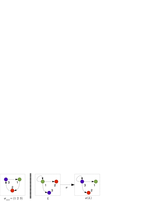
Figure 7: Example of Permutation (Left) and its Associated Production (Right)

Example.$\square$Suppose we are given the permutation $\sigma=(1\;2\;3)\in S_{3}$ to be applied to the graph $L$, depicted to the right of Fig. 7. The associated permutation matrix is

$$\sigma=\left[\begin{array}[]{ccc}\vspace{-4pt}0&1&0\\ \vspace{-4pt}0&0&1\\ \vspace{-4pt}1&0&0\\ \vspace{-10pt}\hfil\end{array}\right].$$

Its action is equivalent to a node relabeling where node $1$ plays the role of node $2$, node $2$ that of node $3$ and node $3$ becomes node $1$. If we wanted to put $\sigma$ as an $(e,r)$ production, its erasing and addition matrices would be:

$$e_{\sigma}=\left[\begin{array}[]{ccc}\vspace{-4pt}1&1&1\\ \vspace{-4pt}0&0&0\\ \vspace{-4pt}0&0&0\\ \vspace{-10pt}\hfil\end{array}\right]\qquad r_{\sigma}=\left[\begin{array}[]{ccc}\vspace{-4pt}0&0&0\\ \vspace{-4pt}0&0&0\\ \vspace{-4pt}1&1&1\\ \vspace{-10pt}\hfil\end{array}\right],$$

which have been calculated using eq. (10).

Say we need to relabel node $3$ in Fig. 7 with a new type, for example $4$. It would be possible to proceed in three stages: first add node $4$, then permute nodes $3$ and $4$ applying the 2-cycle $\sigma_{34}=(3\;4)$ – its graph will have nodes $1$ and $2$ with self edges – and then delete node $3$. $\blacksquare$

Despite the possibility of reducing $\odot$ to some $(e,r)$ productions, we shall introduce this new operation, extending the notion of production to that of affine production. The main reason is that, according to eq. (10), the relabeling expressed in terms of $(e,r)$ (as a production) would have different matrices depending on the graph it is applied to. The action of relabeling should have associated a single element, independently of the simple digraph it acts on.

Through concatenation we obtain the two possible combinations of operations $p;\sigma$ and $\sigma;p$, which are respectively:

$$p;\sigma(L) =r\vee\overline{e}\left(\sigma\cdot L\cdot\sigma^{t}\right)$$ (11)

$$\sigma;p(L) =\sigma\cdot\left(r\vee\overline{e}L\right)\cdot\sigma^{t}$$ (12)

We shall be more interested in the combination of both $\sigma;p;\sigma$ – permute the graph, apply production and permute the result. It is readily seen that

$$p^{\sigma}(L)=\sigma;p;\sigma(L) =\sigma\cdot\left[r\vee\overline{e}\left(\sigma\cdot L\cdot\sigma^{t}\right)\right]\cdot\sigma^{t}=\left[\sigma\cdot\left(r\vee\overline{e}\right)\cdot\sigma^{t}\right]L,$$ (13)

which defines the action $\rho_{\sigma}$ of eq. (9) for productions. Equation (13) can be rewritten $p^{\sigma}(L)=\langle L,\sigma.\,p\rangle$.

Definition 10 (Affine Production)

A production $p:L\rightarrow R$ as defined by eq. (13) is dynamically represented by

$$p=(L,K,e,r,\sigma,\lambda)$$ (14)

where $L$ is the LHS, $K$ is the labeled simple digraph associated to the nihilation matrix, $e$ is the deletion matrix, $r$ is the addition matrix, $\sigma$ is a relabeling and $\lambda$ is the node labeling mapping.

Clearly, making $\sigma$ the identity returns an $(e,r)$ production (which will be known as the traslational part of the affine production) and setting $e=r=\mathbf{0}$ transforms the production in a pure relabeling action (which will be known as the rotational part of the affine production).

Proposition 1

The action on productions $\rho_{\sigma}(p)=p^{\sigma}$ is an homomorphism when the concatenation operation is considered.

Proof
$\square$We have to check the following three properties:

1. $\rho_{\sigma}(\mathbf{1})=\mathbf{1}$.

2. $\rho_{\sigma}(p_{2};p_{1})=\sigma;p_{2};p_{1};\sigma=\sigma;p_{2};\sigma;\sigma;p_{1};\sigma=\rho_{\sigma}(p_{2});\rho_{\sigma}(p_{1})$.

3. $\rho_{\sigma}\left(p^{-1}\right)=\sigma;p^{-1};\sigma=\left(\sigma^{-1};p;\sigma^{-1}\right)^{-1}=\left(\sigma;p;\sigma\right)^{-1}=\left[\rho_{\sigma}\left(p\right)\right]^{-1}$. $\blacksquare$

4 Formal Grammar

In this section we give a definition of MGG as a formal grammar and postpone its study as a model of computation to the next section.

In this author’s opinion, the main drawback to approach the PvsNP problem (complexity theory in general) is the lack of branches of mathematics available. The motivation to introduce MGG as a formal grammar is to pose an algebraic approach to complexity theory. This is done prior to its definition as a model of computation to make the link more evident.

The exposition moves from the abstract to the concrete. Recall that a formal grammar is the quad-tuple $\left(\mathcal{N},\Sigma,\mathcal{P},s_{0}\right)$, being $\mathcal{N}$ a finite set of non-terminal symbols, $\Sigma$ a finite set of terminal symbols $\left(\mathcal{N}\cap\Sigma=\emptyset\right)$, $\mathcal{P}$ a finite set of production rules and $s_{0}\in\mathcal{N}$ the start symbol. Production rules have the general form

$$\left(\Sigma\cup\mathcal{N}\right)^{*}\mathcal{N}\left(\Sigma\cup\mathcal{N}\right)^{*}\longrightarrow\left(\Sigma\cup\mathcal{N}\right)^{*},$$ (15)

where ^∗ is the Kleene star operator. See for example [7]. Equation (15) demands at least one non-terminal symbol on the LHS. The operations on chains of symbols are concatenation and non-terminal symbol replacement, the latter defined through production rules. We shall dedicate the rest of the section to these two operations.

We shall start with the set of $n\times n$ matrices over the field $\mathbb{Z}_{2}[i]$, $M_{n}\left(\mathbb{Z}_{2}[i]\right)$. An element $z=x+iy\in\mathbb{Z}_{2}[i]$ is such that $x,y\in\{0,1\}$. We shall consider the following operations over $M_{n}\left(\mathbb{Z}_{2}[i]\right)$:

1. Multiplication by scalars. Represented by $\cdot$. As we are in $\mathbb{Z}_{2}$, this operation either lets the element unaltered or transforms it into the zero matrix $\mathbf{0}$.

2. Matrix addition. Represented by $+$ and defined in the usual way.

3. Matrix multiplication. Represented by $\odot$ or by $\cdot$ if no confusion with the multiplication by scalars may rise. Defined as usual, with addition and multiplication carried out over $\mathbb{Z}_{2}$.

4. Pointwise multiplication. Represented by $\wedge$ (omitted by default). Let be given $\mathcal{L},\mathcal{R}\in M_{n}\left(\mathbb{Z}_{2}[i]\right)$ with $\mathcal{L}=L+iK$ and $\mathcal{R}=R+iQ$, then

   $$\mathcal{L}\wedge\mathcal{R}=\mathcal{L}\mathcal{R}=(LR+KQ)+i(LQ+KR)$$ (16)

   where $XY$ is the elementwise multiplication, $XY=\left(x^{j}_{m}y^{j}_{m}\right)_{j,m\in\{1,\ldots,n\}}$.

5. Scalar product. Let $\mathcal{L}_{j}=L_{j}+iK_{j}\in M_{n}\left(\mathbb{Z}_{2}[i]\right)$, then the scalar product is represented by $\left\langle\mathcal{L}_{1},\mathcal{L}_{2}\right\rangle$ and defined if

   $$(L_{1}+K_{1})(\mathbf{1}+L_{2}+K_{2})=0.$$ (17)

   This condition guarantees that $\mathcal{L}_{1},\mathcal{L}_{2}\in M_{n}\left(\mathbb{Z}_{2}[i]\right)\implies\left\langle\mathcal{L}_{1},\mathcal{L}_{2}\right\rangle\in M_{n}\left(\mathbb{Z}_{2}[i]\right)$. See the proof of Prop. 2 on p.2.

As we shall be almost exclusively interested in those elements that have disjoint real and imaginary parts, let’s introduce

$$\widetilde{\mathbb{M}}^{n}=\left\{\mathcal{L}=L+iK\in M_{n}\left(\mathbb{Z}_{2}[i]\right)\;\left|\;LK=0\right.\right\}.$$ (18)

Elements of $\widetilde{\mathbb{M}}^{n}$ will be known as Boolean complex matrices. Let $\mathcal{T}$ be some finite set and for $\tilde{g}\in\widetilde{\mathbb{M}}^{n}$ consider the mapping $\lambda_{\tilde{g}}:\tilde{g}\rightarrow\mathcal{T}$ defined only for elements in the diagonal of $L$ and $K$ and such that $\lambda(L)=\lambda(K)$. The meaning of $\lambda$ will be clarified in Sec. 5. Its subscript will be usually omitted.

Except for some restrictions on the operations – their concrete definition taking $\lambda$ into account are given in eqs. (22), (23) and (3) below – the (vector) space on which we shall focus our attention is $\left(\mathbb{M}^{n},+,\cdot\,,\odot\right)$, where

$$\mathbb{M}^{n}=\left\{g=\left(\tilde{g},\lambda\right)\;\left|\;\tilde{g}\in\widetilde{\mathbb{M}}^{n}\textrm{ and }\lambda\textrm{ as above}\right.\right\}.$$ (19)

For MGG, the quad-tuple $\mathfrak{G}=\left(\mathcal{N},\Sigma,\mathcal{P},s_{0}\right)$ that defines the formal grammar has the following elements:

• $\mathcal{N}=\left\{\mathcal{L}_{i}\;|\;\exists p_{i}:\mathcal{L}_{i}\rightarrow\mathcal{R}_{i},\;p_{i}\in\mathcal{P}\right\}$, the finite set of elements in $\mathbb{M}^{n}$ that appears in the LHS of some production rule.

• $\Sigma=\left\{\mathcal{L}\in\mathbb{M}^{n}\;|\;\mathcal{L}\not\in\mathcal{N}\right\}$, the finite set of elements in $\mathbb{M}^{n}$ not belonging to $\mathcal{N}$.

• $\mathcal{P}=\left\{p:\mathcal{L}\rightarrow\mathcal{R}\;|\;\mathcal{L}\in\mathcal{N},\;\mathcal{R}\in\Sigma\cup\mathcal{N}\right\}$, the finite set of production rules as defined in eq. (20) below.

• $S_{0}\in\mathbb{M}^{n}$, the start symbol.

MGG as a formal grammar (and as a model of computation) will be limited to “affine” mappings, which correspond to non-terminal symbol replacement (concatenation is addressed by the end of the section). A grammar rule $p$ has the general form

$$\mathcal{S}_{1}=p(\mathcal{S}_{0})=\left\langle S_{0},\sigma.\,\omega\right\rangle=\left\langle\mathcal{S}_{0},\sigma\cdot\omega\cdot\sigma^{t}\right\rangle,$$ (20)

where $\mathcal{S}_{0},\mathcal{S}_{1}\in\mathbb{M}^{n}$, $\sigma$ is a permutation matrix (a single $1$ per row and column; see Sec. 3) and $\omega\in\mathbb{M}^{n}$ is such that there exists $\alpha\in\mathbb{M}^{n}$ with zero imaginary part that fulfills

$$\omega=\alpha+i(\alpha+\mathbf{1}),$$ (21)

being $\mathbf{1}\in\mathbb{M}^{n}$ the $n\times n$ matrix filled up with ones (by eq. (18) the imaginary part must be zero). These elements have been introduced in [17], so-called swaps.

The way operations in eqs. (20) and (21) are carried out need to be clarified regarding the $\lambda$ mappings, which are part of the elements of $\mathbb{M}^{n}$ according to (19):

1. Multiplication by scalars is defined by

   $$\alpha\mathcal{L}=\left(\alpha L+i\alpha K,\lambda(\mathcal{L})\right),\qquad\alpha=0,1.$$ (22)

2. The addition $\mathcal{L}_{1}+\mathcal{L}_{2}$ should respect the mapping $\lambda$ so it is allowed just in case $\lambda_{\mathcal{L}_{1}}(\mathcal{L}_{1})=\lambda_{\mathcal{L}_{2}}(\mathcal{L}_{2})$:

   $$\mathcal{L}_{1}+\mathcal{L}_{2} =\left((L_{1}+L_{2})+i(K_{1}+K_{2}),\lambda(\mathcal{L}_{1})\right)=$$ (23)

   $$=\left((L_{1}+L_{2})+i(K_{1}+K_{2}),\lambda(\mathcal{L}_{2})\right).$$

3. Recall from Sec. 3 that permutation matrices define a permutation on the indices of the elements of $\mathbb{M}^{n}$, $\sigma(1\;2\;\ldots\;n)=(\sigma(1)\;\sigma(2)\;\ldots\;\sigma(n))$. For $\mathcal{L}\in\mathbb{M}^{n}$ the matrix multiplication is given by

   $$\sigma.\,\mathcal{L}=\sigma\cdot\mathcal{L}\cdot\sigma^{t} =\sigma\cdot(L+iK,\lambda)\cdot\sigma^{t}=$$

   $$=\left(\sigma\cdot(L+iK)\cdot\sigma^{t},\sigma\left(\lambda\left(\mathcal{L}_{jj}\right)\right)\sigma^{t}\right)=$$

   $$=\left(\sigma\cdot L\cdot\sigma^{t}+i\sigma\cdot K\cdot\sigma^{t},\lambda\left(\mathcal{L}_{\sigma(j)\sigma(j)}\right)\right).$$ (24)

The following proposition now follows easily:

Proposition 2

The formal grammar $\mathfrak{G}$ is closed under the operations given by the production rules as defined in eq. (20).

Proof
$\square$The proof can almost be derived from the fact that $\mathbb{M}^{n}$ is closed under the operations $\cdot$, $+$, $\odot$ defined in eqs. (22), (23) and (3):

1. $\alpha=0,1,\;\mathcal{L}\in\mathbb{M}^{n}\implies\alpha\cdot\mathcal{L}\in\mathbb{M}^{n}$ holds because $\mathbf{0}\in\mathbb{M}^{n}$.

2. $\mathcal{L}\in\mathbb{M}^{n},\sigma\textrm{ permutation}\implies\sigma\cdot\mathcal{L}\cdot\sigma^{t}\in\mathbb{M}^{n}$ because it is just a relabeling.

3. $\mathcal{L}_{1},\mathcal{L}_{2}\in\mathbb{M}^{n}\implies L_{1}+L_{2}\in\mathbb{M}^{n}$ because addition respects labeling.

A little of extra work is needed for the scalar product:

$$\left\langle\mathcal{L}_{1},\mathcal{L}_{2}\right\rangle =\left\langle L_{1}+iK_{1},L_{2}+iK_{2}\right\rangle=\left(L_{1}+iK_{1}\right)\left(\mathbf{1}+K_{2}+i(\mathbf{1}+L_{2})\right)=$$

$$=\left(L_{1}+L_{1}K_{2}+K_{\textordmasculine}+K_{1}L_{2}\right)+i\left(K_{1}+K_{1}K_{2}+L_{1}+L_{1}L_{2}\right)=$$

$$=\alpha+i\beta.$$

so $\left\langle\mathcal{L}_{1},\mathcal{L}_{2}\right\rangle\in\mathbb{M}^{n}$ if $\alpha\beta=0$. After some manipulations, we obtain that

$$\alpha\beta=\left(L_{1}+K_{1}\right)\left(\mathbf{1}+L_{2}+K_{2}\right).$$ (25)

To see that eq. (21) guarantees $\alpha\beta=0$ simply substitute it into eq. (25). $\blacksquare$

Concatenation as an operation is simpler than non-terminal symbol replacement. In essence it consists in passing from $\mathbb{M}^{m}$ to $\mathbb{M}^{n}$ with $m\leq n$. Assuming that $\mathcal{T}$ is not enlarged, all we have to do is to add $n-m$ rows and columns to the matrices that define the production rules (filling them with zeros) and consider these new rows and columns in the permutation matrices.

The production rules in $\mathfrak{G}$ have the general form $\mathcal{N}\rightarrow\Sigma\cup\mathcal{N}$, which is a particular case of eq. (15). Taking concatenation into account, the general form that appears in eq. (15) is recovered.

5 Model of Computation

In this section we shall start by informally providing some semantics to the elements and operations of the formal grammar $\mathfrak{G}$ of Sec. 4: elements of $\mathbb{M}^{n}$ (permutation matrices in particular), addition, matrix multiplication, the set $\mathcal{T}$, the mapping $\lambda$ and the element $\omega$ as introduced in eq. (21). After this, the nodeless MGG model of computation is defined. The section is closed with a short summary on some MGG submodels and supermodels of computation.

Let $\mathcal{L}=L+iK\in\mathbb{M}^{n}$. The Boolean matrix $L$ can be seen as the adjacency matrix of some simple digraph $g$. This matrix is completed with $K$, which we will interpret as those edges that can not belong to $g$.

A meaning for $\mathcal{T}$ could be that of (node) labels. Closely related is the mapping $\lambda$ that assigns a label to each node. This is why it is just defined for the elements in the main diagonal. It is natural to impose $\lambda(L)=\lambda(K)$. The operation defined by eq. (3) can be understood as a node relabeling. Refer to Sec. 3.

The definition of $\omega$ given in eq. (21) simply states that we have to do inverse operations on $L$ and $K$ (refer to Sec. 2). The permutation matrix $\sigma$ allows $\omega$ to act on rearrangements of elements equally labeled.

Notice that no restrictions can be set on the applicability of production rules according to eq. (20), i.e. swaps can always be applied. We shall introduce a new means to define productions (as introduced in MGG; see Sec. 2) using the Boolean operations and (pointwise multiplication) and or (close to matrix addition) and the erasing and addition matrices. This will be our model of computation, to be known as nodeless MGG. Productions can be understood as swaps with restrictions: productions are one of the possible ways to set constraints on the applicability of swaps.

The model of computation associated to MGG is the 5-tuple $\left(\mathcal{G},\mathcal{T},\mathcal{P},\tau,H_{0}\right)$ where

• $\mathcal{G}=\left\{\mathcal{L}=(L,K,\lambda)\;\left|\right.\;\lambda:V(\mathcal{L})\rightarrow\mathcal{T}\right\}$, being $V(\mathcal{L})$ the set of vertices. The formal notation $\mathcal{L}=L\vee iK$ will be used.

• $\mathcal{T}$ is the finite set of labels.

• $\mathcal{P}$ is the finite set of compatible productions.

• $\tau$ is the transition function that modifies the state:

  $$\tau:\mathcal{G}\times\mathcal{P} \longrightarrow\mathcal{G}$$

  $$(H,p) \longmapsto\langle H,p\rangle=p(H)=H^{\prime}$$

• $H_{0}$ is the initial system state (see Sec. 2).

The model is deterministic if $\tau$ is a single-valued function and non-deterministic if it is a multivalued function. The default halting condition is “no production can be applied”.

The two basic operations are again non-terminal symbol replacement and concatenation, on which we touch in the following paragraphs.

Concatenation in MGG is defined for productions, which is just the sequential application of two or more productions. It will be represented by a semicolon and should be read from right to left (like standard composition of functions). Refer to Sec. 2 for more details.

Graph rewriting substitutes the occurrence of some graph (known as pattern graph or production LHS, $L$) in the host graph $(H)$ by the corresponding replacement graph (also known as production RHS, $R$). The specification of the operation is done through a so-called grammar rule, production rule or just production, and is represented as a graph morphism $p:L\rightarrow R$. The operation itself is known as a derivation. Refer again to Sec. 2. Graph rewriting plays in MGG the role of non-terminal symbol replacement in formal grammars.

We can associate the element $p=e\vee ir$ to any production $p$, being $e$ and $r$ their erasing and addition matrices, respectively, which have been introduced in Sec. 2. Notice that as $e$ and $r$ are disjoint, the or and the matrix addition coincide, so we can think of $p$ as an element of $\mathbb{M}^{n}$.

From the element $p=e\vee ir$ we can define a swap $\omega=P(p)=P(e\vee ir)=\overline{e}\,\overline{r}\vee i(e\vee r)$. Again, as $\overline{e}\,\overline{r}$ and $e\vee r$ are disjoint we can write

$$\omega=(e+\mathbf{1})(r+\mathbf{1})+i(e+r)=(e+r+\mathbf{1})+i(e+r).$$ (26)

Notice that $\omega$ satisfies eq. (21), hence the name. Moreover, as was proved in [18], $R=\left\langle L,P(p)\right\rangle$. Taking relabeling into account we can write an affine production as

$$R\vee iQ=\mathcal{R}=p(\mathcal{L}) =\sigma\cdot\left\langle\sigma\cdot(L\vee iK)\cdot\sigma^{t},\overline{e}\,\overline{r}\vee i\left(e\vee r\right)\right\rangle\cdot\sigma^{t}=$$

$$=\left\langle L\vee iK,\sigma\cdot\left[\overline{e}\,\overline{r}\vee i\left(e\vee r\right)\right]\cdot\sigma^{t}\right\rangle,$$ (27)

which is just eq. (13) including the nihil parts $K$ and $Q$.

The application of the production $p$ to a host graph $G$ to derive the system state $H$ is given by:

$$H=p(G)=\left\langle G,\sigma.\,P(p)\right\rangle.$$ (28)

The matching – see Chap. 6 in [16] – is performed by the relabeling $\sigma$. Notice the non-determinism of this step and its NP-completeness. Compare with eq. (20).

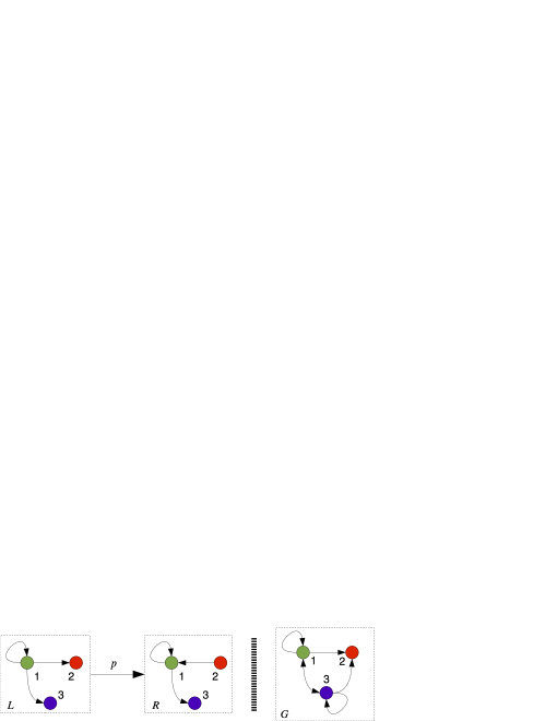
Figure 8: Sample Permutation plus Host Graph

Example.$\square$Let’s consider the production $p$ and the host graph $G$ depicted in Fig. 8. The nihil terms $K$ and $Q$ have been omitted to ease exposition. All nodes are assumed to be of the same type so neither the numbers nor the colors in the figure should be understood as labels. Numbers are used for referencing purposes only.

Production $p$ deletes edge $(1,2)$ and adds a new edge $(2,1)$. It also keeps edges $(1,1)$ and $(1,3)$, demanding their existence in the host graph. There are initially four possible identifications of the LHS $L$ in $G$, which correspond to the following mappings: $(1,2,3)\longmapsto(1,2,3),(1,3,2),(3,2,1)$ and $(3,1,2)$. The permutation matrices are

$$\sigma_{1}=\left[\begin{array}[]{ccc}\vspace{-4pt}1&0&0\\ \vspace{-4pt}0&1&0\\ \vspace{-4pt}0&0&1\\ \vspace{-10pt}\hfil\end{array}\right]\quad\sigma_{2}=\left[\begin{array}[]{ccc}\vspace{-4pt}1&0&0\\ \vspace{-4pt}0&0&1\\ \vspace{-4pt}0&1&0\\ \vspace{-10pt}\hfil\end{array}\right]\quad\sigma_{3}=\left[\begin{array}[]{ccc}\vspace{-4pt}0&0&1\\ \vspace{-4pt}0&1&0\\ \vspace{-4pt}1&0&0\\ \vspace{-10pt}\hfil\end{array}\right]\quad\sigma_{4}=\left[\begin{array}[]{ccc}\vspace{-4pt}0&0&1\\ \vspace{-4pt}1&0&0\\ \vspace{-4pt}0&1&0\\ \vspace{-10pt}\hfil\end{array}\right]$$

with associated productions

$$q_{i}(L)=\langle L,\sigma_{i}.\,p\rangle=\langle L,\sigma_{i}\cdot p\cdot\sigma_{i}^{t}\rangle,\quad i\in\{1,2,3,4\}.$$

In principle, all four are valid productions but not all can be applied to $G$. Production $p_{2}$ would try to add edge $(3,1)$ which already exists in $G$. The same problem appears with $p_{4}$ but this time with edge $(1,3)$.

Apart from illustrating how relabeling works on productions, this example tries to show how it will be of help in characterizing non-determinism in Sec. 6. $\blacksquare$

The main difference between what is exposed in this section and Sec. 2 is that nodeless MGG does not act on nodes but just on edges. This has the advantage of avoiding dangling edges and all compatibility issues derived.

The section ends brushing over submodels (by setting further constraints on MGG) and supermodels of computation (by relaxing the axioms of nodeless MGG). An initial proposal is:

1. On the matching:

   • For submodels, a subisomorphism instead of an injective morphisms – as in Def. 9 – can be demanded.

   • As a supermodel, the injectivity of the morphism may be relaxed.

2. On the productions:

   • For submodels, relabeling can be forbidden. Other constraints on the operations can be set by using application conditions (see [16], Chaps. 8 and 9).

   • Nodeless MGG can be extended by allowing graph constraints and application conditions (see [16]). Also, new operations on graphs can be allowed such as negation of graphs or we can permit general adjacency matrices in the multiplication instead of just permutational matrices (see Prop. 3 below).

3. On the underlying space:

   • For submodels, instead of considering simple digraphs we may consider undirected graphs or even subsets such as the group of permutations (digraphs with single incoming and outgoing edges).

   • Other structures more general than simple digraphs can be allowed. Examples are multidigraphs and hypergraphs.

Limiting matrix multiplication to permutation matrices is a big restriction, at least concerning the amount of matrices left out. The following proposition shows the orders as functions on the number of nodes:

Proposition 3

Assuming that all nodes are of the same type, the orders of the number of permutation matrices per swap $P_{\omega}(n)$ and per production $P_{p}(n)$ are:

$$P_{\omega}(n)=\frac{\#(\mathtt{perms})}{\#(\mathtt{swaps})}=\frac{n!}{2^{n^{2}}} \sim\frac{\sqrt{\pi n}\left(\frac{n}{e}\right)^{n}}{2^{n^{2}-1/2}}\in e^{-O\left(n^{2}\right)},$$ (29)

$$P_{p}(n)=\frac{\#(\mathtt{perms})}{\#(\mathtt{prods})}=\frac{n!}{3^{n^{2}}} \sim\frac{\sqrt{2\pi n}\left(\frac{n}{e}\right)^{n}}{3^{n^{2}}}\in e^{-O\left(n^{2}\right)},$$ (30)

where $n$ is the number of nodes.

Proof
$\square$Recall that $\log_{b}(x)=\frac{\log_{c}(x)}{\log_{c}(b)}$. The Stirling formula for the factorial (the number of permutations) has been used in eqs. (29) and (30). For the denominator, notice that a swap is fixed by its real or imaginary parts, so there are as many as adjacency matrices for graphs with $n$ nodes: $2^{n^{2}}$. To prove eq. (29) just take the logarithms to derive

$$\frac{\log(2)+\log{\pi}}{2}+\frac{\log(n)}{2}-n+n\log(n)-\log(2)n^{2}.$$ (31)

All we have to do to check eq. (30) is to count the number of different productions that can be defined for graphs with $n$ nodes. One possibility is to establish a link between productions and the standard Sierpinski gasket. To this end, write the adjacency matrix of the graph $g$ of $n$ nodes as a single column (the second sitting right after the first, the third after the second and so on). Recall that a production $p$ can be written as $p=e\vee ir$, with $er=0$. Hence, productions are the zeros of the and function. See Fig. 9 which represents well defined productions of the form $p=e\vee ir$ for matrices with two nodes.

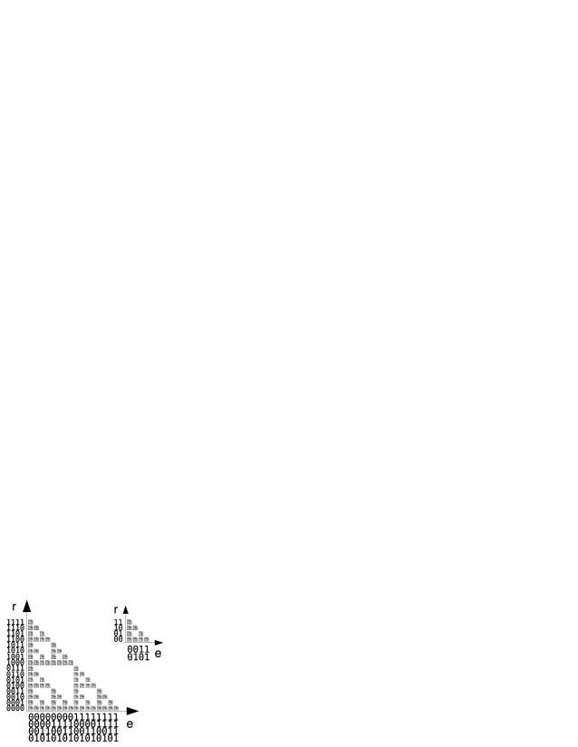
Figure 9: Weel-Defined Productions

The Lucas correspondence theorem (see [5] and also [23]) proves that the set of zeros is the Sierpinski gasket as it can be used to compute the binomial coefficient $\binom{L}{K}\mod 2$ with bitwise operations: $\overline{L}\wedge K$. This tells us that the parity of the function $\binom{L}{K}$ (this is what the function $\!\!\!\!\mod 2$ does) is the same as that of $\overline{L}\wedge K$. In our case $L$ is the abscissa. The negation of $L$ just reverts the order (it is a symmetry) and does not change the shape of the figure.

Counting the number of elements is not difficult. Notice that in Fig. 9, the big Sierpinsky gasket is made of a number of copies of the smaller one. The small Sierpinsky gasket has $9$ elements and it appears $3^{n^{2}-2}$ times so the total amount of well defined productions is $3^{n^{2}}$. The main difference with respect to eq. (31) is the coefficient of $-n^{2}$ which would be $\log(3)$ this time. $\blacksquare$

6 Determinism and Non-Determinism in MGG

There are two types (sources) of non-determinism associated to the grammar state: selecting the next production to apply (let’s call it election non-determinism) and finding the place in the host graph where the production will be applied (that we shall name allocation non-determinism). The transition function is not uniquely determined either because more than one production can be applied or because the oracle returns more than one place where the production can be applied.

One easy way to mitigate or to even remove non-determinism is to use control nodes that indicate what production to apply or where it should be applied. Examples of these control nodes are the $S_{i}$ that appear in the productions of Sec. 8, Figs. 14, 15 and 16. It is also possible that, for certain purposes, which production is applied or where it is applied becomes irrelevant. An example of this behavior is the simulation of BCs given in Sec. 9.

Figure 10: Productions Application (Derivation: Evolution of a System)

If a sequence of productions $s=p_{n};\ldots;p_{1}$ (see Fig. 10) is considered instead of a single production, allocation non-determinism can be graded. There is a first partial level where only productions are taken into account (ignoring the initial and intermediate system states) and a second complete level if the host graphs are considered. Let’s call them horizontal non-determinism and vertical non-determinism, respectively.

Remark.$\square$The names stem from the way the identification of elements is performed according to the representation in Fig. 10. If the system states are not taken into account, the identification of nodes is horizontal (in productions $p_{i}$). If the system states are considered, the identifications are given by the matching mappings $m_{i}$. $\blacksquare$

Nodes with the same label are potentially interchangeable so non-determinism in a single graph is equivalent to the Cartesian product of the corresponding permutation groups (one per type). For a given simple digraph $L$, let’s denote this group by $S(L)$. Their elements are represented by permutation matrices as explained in Sec. 3.

An affine production $p:L\rightarrow R$ identifies nodes between $L$ and $R$ in a unique way. The traslational part of the production that acts on edges does not affect the permutation group of the RHS. The rotational part $\sigma$ does not affect the permutation group of the RHS either:

$$\mathcal{S}(R)=\{\sigma\cdot\sigma_{i}\,|\,\sigma_{i}\in\mathcal{S}(L)\}=S(L).$$

Hence, productions in nodeless MGG do not modify the permutation group associated to graphs.

Horizontal non-determinism in sequences can be handled by letting the permutational part of productions vary in the corresponding permutation group. Notice however that not all variations are possible if applicability is to be kept (see the example of Fig. 8).

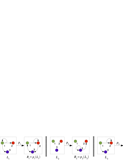
Figure 11: Sample Productions

Example.$\square$Let’s consider the productions $p_{1}$, $p_{2}$ and $p_{3}$ depicted in Fig. 11, being $1$, $2$ and $3$ nodes of the same type. The group of permutations of three elements is $S_{3}=\{id,(1\;2),(1\;3),(2\;3),(1\;2\;3),(3\;2\;1)\}$. Their associated affine productions are

$$q^{\sigma}_{i}(L_{i})=\left\langle L_{i},\sigma.\,p_{i}\right\rangle=\left\langle L_{i},\sigma\cdot p_{i}\cdot\sigma^{t}\right\rangle,\quad i\in\{1,2,3\},$$

with $\sigma\in S_{3}$. The sequence $s=p_{3};p_{2};p_{1}$ has associated affine sequence

$$s^{\prime}=q_{3};q_{2};q_{1}=\langle\langle\langle L_{1},\sigma^{1}\!\!.\,p_{1}\rangle,\sigma^{2}\!\!.\,p_{2}\rangle,\sigma^{3}\!\!.\,p_{3}\rangle.$$

$I^{I^{I}}$$\sigma^{2}\backslash\sigma^{1}$$I^{I^{I}}$	$\;\;\;id\;\;\;$	$\,\;(1\;2)\;\,$	$\,\;(1\;3)\;\,$	$\,\;(2\;3)\;\,$	$\,(1\;2\;3)\,$	$\,(3\;2\;1)\,$
$id$	1	0	0	0	0	0
$(1\;2)$	0	1	0	0	0	0
$(1\;3)$	0	0	1	0	0	0
$(2\;3)$	0	0	0	1	0	0
$\,(1\;2\;3)\,$	0	0	0	0	1	0
$\,(3\;2\;1)\,$	0	0	0	0	0	1

Table 1: Possible Relabelings for Sequence $s=p_{2};p_{1}$

Table 1 includes all the permutations for the subsequence $p_{2};p_{1}$. A $1$ means that applicability is kept and a $0$ means that applicability is not kept. Only the diagonal keeps applicability. The problem in all cases is that some already existing edge would be added by $q_{2}$.

$I^{I^{I}}$​​ $\sigma^{3}\backslash\sigma^{2}\sigma^{1}$ $I^{I}$	$[id,\!id]$	$[(1\,2),\!(1\,2)]$	$[(1\,3),\!(1\,3)]$	$[(2\,3),\!(2\,3)]$	$[(1\,2\,3),\!(1\,2\,3)]$	$[(3\,2\,1),\!(3\,2\,1)]$
$id$	1	0	1	1	0	0
$(1\;2)$	0	1	0	0	1	1
$(1\;3)$	1	0	1	0	0	1
$(2\;3)$	1	0	0	1	1	0
$\,(1\;2\;3)\,$	0	1	0	1	1	0
$\,(3\;2\;1)\,$	0	1	1	0	0	1

Table 2: Possible Relabelings for Sequence $s=p_{3};p_{2};p_{1}$

Table 2 summarizes all permutations for the sequence $p_{3};p_{2};p_{1}$. Just the permutations that keep applicability for $p_{2};p_{1}$ has been considered (indexed by columns). Again, a $1$ means that applicability is kept and a $0$ means that applicability is not kept. The problem in all cases is that some non-existent edge would be deleted by $q_{3}$.

In this example, as there are many possible relabelings, we have that the sequence is horizontally non-deterministic. Figure 12 represents the effect of applying the sequence $s=q^{(1\;2\;3)}_{3};q^{(1\;2)}_{2};q^{(1\;2)}_{1}$ to the initial host graph $L_{1}$. $\blacksquare$

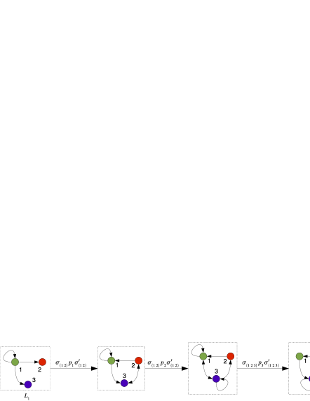
Figure 12: Image of the Sequence of Three Productions

Proposition 4 (Horizontal Determinism Characterization)

Let $s_{n}=p_{n};\ldots;p_{1}$ be a compatible sequence of productions and define the operator $\widetilde{C}(s_{n})=\widetilde{C}^{+}(s_{n})\vee\widetilde{C}^{-}(s_{n})$ by

$$\widetilde{C}^{+}(s_{n}) =\bigvee_{j=1}^{n}\left(R^{\sigma}_{j}\underset{j+1}{\overset{n}{\nabla^{\prime}}}\left(\overline{e}^{\sigma}_{x}\,r^{\sigma}_{y}\right)\vee L^{\sigma}_{j}\underset{1}{\overset{j-1}{\bigtriangleup}}\left(e^{\sigma}_{y}\,\overline{r}^{\sigma}_{x}\right)\right)$$ (32)

$$\widetilde{C}^{-}(s_{n}) =\bigvee_{i=1}^{n}\left(Q^{\sigma}_{i}\underset{j+1}{\overset{n}{\nabla^{\prime}}}\left(\overline{r}^{\sigma}_{x}\,e^{\sigma}_{y}\right)\vee K^{\sigma}_{i}\underset{1}{\overset{j-1}{\bigtriangleup^{\prime}}}\left(\overline{e}^{\sigma}_{x}\,r^{\sigma}_{y}\right)\right),$$ (33)

being $X_{i}^{\sigma}=\sigma_{i}.\,X_{i}=\sigma_{i}\cdot X_{i}\cdot\sigma^{t}_{i}$, $X_{i}=e_{i},r_{i},L_{i},R_{i},K_{i},Q_{i}$, and

$$\underset{t_{0}}{\overset{t_{1}}{\bigtriangleup^{\prime}}}\left(F(x,y)\right)=\bigvee_{y=t_{0}}^{t_{1}}\left(\bigwedge_{x=y}^{t_{1}}\left(F(x,y)\right)\right),\;\underset{t_{0}}{\overset{t_{1}}{\nabla^{\prime}}}\left(F(x,y)\right)=\bigvee_{y=t_{0}}^{t_{1}}\left(\bigwedge_{x=t_{0}}^{y}\left(F(x,y)\right)\right).$$

There are three possibilities:

1. The sequence is not applicable if for some $i$ there exists no permutation such that $\widetilde{C}(s_{n})=\mathbf{0}$.

2. The sequence is horizontally deterministic if for every $i$ there exists a single permutation such that $\widetilde{C}(s_{n})=\mathbf{0}$.

3. The sequence is horizontally non-deterministic if for some $i$ there exists more than one possible permutation $\sigma$ such that $\widetilde{C}(s_{n})=\mathbf{0}$.

Proof (sketch)
$\square$Theorem. 6.4.4 in [16] characterizes applicability as equivalent to compatibility plus coherence. Applicability in a single place is determinism and applicability in several places is non-determinism. Compatibility is always fulfilled by nodeless MGG and nevertheless a hypothesis of the proposition, so it just remains to study coherence.

Equations (32) and (33) for productions instead of affine productions characterizes coherence as proved in Th. 2, Sec. 5 in [18], or in Theorems 4.3.5 and 4.4.3 in [16]. To finish the proof, simply add permutations to the productions (to tackle relabeling) transforming them into affine productions. $\blacksquare$

We shall end this section by pointing out that vertical non-determinism can be addressed as horizontal non-determinism. The only difference is that matrices (and thus permutation groups) will be larger.

7 From Boolean Algebra to a Matrix Algebra

Matrix Graph Grammars use Boolean algebra mainly because production actions and graphs are characterized through Boolean matrices and Boolean operations (and and or). As swaps are linear transformations, it seems interesting to move to algebra and try to identify the linear operations (if any). The first thing to do is to recover productions from swaps.

Recall that a swap can be applied to any host graph whereas for a production we need to find some elements in the host graph $(L)$ and guarantee that some others $(K)$ are not present: a production is a swap together with some restrictions.

Proposition 5

Let $p=(\mathcal{L},e+ir)=(L+iK,e+ir)$ be as in previous sections a production and $\omega=P(p)=(e+r+\mathbf{1})+i(e+r)$ its associated swap, applied to the host graph $G$. The image of the production – $\mathcal{R}=p(\mathcal{L})$ – is given by:

$$\begin{cases}H=p(G)=\sigma.\,\omega+G&\mbox{(graph transformation)}\\ QR=(\sigma.K)G=(\sigma.L)(G+\mathbf{1})=\mathbf{0}&\mbox{(application conditions)}\end{cases}$$

Proof
$\square$According to Prop. 4 the application can be deterministic, non-deterministic or impossible, depending on $\sigma$. In [16], Chap. 6, it is proved that a direct derivation can be defined (equiv., a production can be applied) if the production is well-defined (compatible) and its LHS is found in the host graph (and the nihilation matrix is not present in the host graph).

The first application condition $QR=0$ is compatibility. If we limit ourselves to nodeless MGGs, this condition will be always fulfilled. The second condition demands the non-existence of $K$ in $G$. It is equivalent to $(\sigma.K)(G+\mathbf{1})=\sigma.K$. The third condition demands the existence of $L$ in $G$ as it is equivalent to $(\sigma.L)G=\sigma.L$. $\blacksquare$

Remark.$\square$The graph transformation part is linear while the application condition part is non-linear. Application conditions and their generalizations (so-called graph restrictions) are studied in [19], and also in Chaps. 8 and 9 in [16]. $\blacksquare$

The next step is to characterize the application of a sequence with a finite number of productions, $s=p_{n};\ldots;p_{1}$. There will be again two parts, one linear with the actions and one non-linear with the restrictions (see Th. 7.1 below). In particular we shall guarantee in the propositions that follow that the sequence is compatible, coherent and that the initial digraph is contained in $G+i(G+\mathbf{1})$, being as always $G$ the host graph.

Proposition 6

With notation and hypothesis as in Prop.  4, the same conclusions hold if the operator $C(s)=C^{+}(s)+iC^{-}(s)$ that assigns one element of $\mathbb{M}^{n}$ to the sequence $s$ is considered:

$$C^{+}(s)=1+\prod_{j=1}^{n} \left(R^{\sigma}_{j}\underset{j+1}{\overset{n}{\nabla}}\left[\left(e^{\sigma}_{x}+\mathbf{1}\right)r^{\sigma}_{y}\right]+L^{\sigma}_{j}\underset{1}{\overset{j-1}{\bigtriangleup}}\left[\left({r}^{\sigma}_{x}+\mathbf{1}\right)e^{\sigma}_{y}\right]+\right.$$

$$+\left.L_{j}^{\sigma}R_{j}^{\sigma}\underset{j+1}{\overset{n}{\nabla}}\left(e^{\sigma}_{x}+\mathbf{1}\right)r^{\sigma}_{y}\underset{1}{\overset{j-1}{\bigtriangleup}}\left({r}^{\sigma}_{x}+\mathbf{1}\right)e^{\sigma}_{y}\right),$$ (34)

$$C^{-}(s)=\mathbf{1}+\prod_{j=1}^{n} \left(Q^{\sigma}_{j}\underset{j+1}{\overset{n}{\nabla}}\left[\left(r^{\sigma}_{x}+\mathbf{1}\right)e^{\sigma}_{y}\right]+K^{\sigma}_{j}\underset{1}{\overset{j-1}{\bigtriangleup}}\left[\left(e^{\sigma}_{x}+\mathbf{1}\right)r^{\sigma}_{y}\right]+\right.$$

$$+\left.K^{\sigma}_{j}Q^{\sigma}_{j}\underset{j+1}{\overset{n}{\nabla}}\left(r^{\sigma}_{x}+\mathbf{1}\right)e^{\sigma}_{y}\underset{1}{\overset{j-1}{\bigtriangleup}}\left(e^{\sigma}_{x}+\mathbf{1}\right)r^{\sigma}_{y}\right),$$ (35)

being

$$\underset{t_{0}}{\overset{t_{1}}{\bigtriangleup}}F(x,y) =\mathbf{1}+\prod_{y=t_{0}}^{t_{1}}\left(\mathbf{1}+\prod_{x=y}^{t_{1}}F(x,y)\right),$$

$$\underset{t_{0}}{\overset{t_{1}}{\nabla}}F(x,y) =\mathbf{1}+\prod_{y=t_{0}}^{t_{1}}\left(\mathbf{1}+\prod_{x=t_{0}}^{y}F(x,y)\right).$$

Proof
$\square$ All we have to do to apply Prop. 4 is to prove the equivalence between equations (32) and (33) and equations (34) and (6), respectively. Also, we have to check sameness of $\bigtriangleup^{\prime}$ and $\nabla^{\prime}$ in Prop. 4 with $\bigtriangleup$ and $\nabla$ in this Proposition. To this end, simply use the following identities from propositional logics:

$$x_{j}\wedge x_{k}=x_{j}\cdot x_{k},\qquad\bigvee_{j=1}^{n}x_{j}=1+\prod_{j=1}^{n}\left(1+x_{j}\right),\qquad\overline{x}=1+x.$$

Both cases $C^{+}$ and $C^{-}$ are almost equal. $\blacksquare$

A similar reasoning applies to the calculation of the initial digraph of a coherent sequence and its compatibility in the following two propositions. as cmomented above, they will be used to characterize determinism of a sequence of productions.

Proposition 7

Let $s=p_{n};\ldots;p_{1}$ be a coherent sequence with notation as above. Then, the initial digraph is given by:

$$M(s)=M_{C}(s)+iM_{N}(s)=\underset{1}{\overset{n}{\nabla}}\left[\left(r^{\sigma}_{x}+\mathbf{1}\right)L^{\sigma}_{y}+i\left(e^{\sigma}_{x}+\mathbf{1}\right)\left(T^{\sigma}_{x}+\mathbf{1}\right)K^{\sigma}_{y}\right].$$ (36)

Proof
$\square$ $\blacksquare$

Proposition 8

Let $s=p_{n};\ldots;p_{1}$ be a sequence made up of compatible productions. Then, $s$ is compatible if $W(s)=\mathbf{0}$, where

$$W(s)=\underset{1}{\overset{n}{\nabla}}\left[\left(e^{\sigma}_{x}+\mathbf{1}\right)\left(r^{\sigma}_{x}+\mathbf{1}\right)M_{C}(s_{x})M_{N}(s_{x})\right].$$ (37)

Proof
$\square$ $\blacksquare$

Previous propositions allow us to characterize determinism – notice that determinism extends applicability as introduced in [16], Chap. 1 –. According to Th. 6.4.4 in [16] all we need is compatibility and coherence of the productions plus finding the initial digraph in $G+i(G+\mathbf{1})$.

Theorem 7.1

Let $s=p_{n};\ldots;p_{1}$ be a sequence of productions with associated swaps $\omega_{j},j=1,\ldots,n$. The image $H$ of the sequence when applied to the host graph $G$ is given by:

$$\begin{cases}H=s(G)=\sum_{j=1}^{n}\sigma_{j}.\,\omega_{j}+G&\mbox{(graph transformation)}\\ W(s)=C(s)=M_{N}(s)G=M_{C}(s)(G+\mathbf{1})=\mathbf{0}&\mbox{(application conditions)},\end{cases}$$

being $M(s)$ the initial digraph, $W(s)$ the compatibility conditions and $C(s)$ the coherence conditions.

Proof
$\square$ $\blacksquare$

If we stick to nodeless MGG then the formulas get simpler as $D_{i}+\mathbf{1}=T_{i}=\mathbf{0}$ and $K_{i}=r_{i},i\in\{1,\ldots,n\}$. Again, the graph transformation part is linear while the part of the application conditions is non-linear.

8 MGG and Turing Machines

In this section the relationship between Matrix Graph Grammars and Turing machines (TM) is studied. Two standard introductions to TMs are [7] and [21]. We will see how to simulate a TM using nodeless MGG. The simulation of TMs using MGG is easy except that the tape in TMs is unbounded.

According to [21], a Turing machine can be formally defined as a finite-state machine with a memory medium. It is the 7-tuple

$$M=\left(Q,\Gamma,\Sigma,\tau,q_{0},q_{a},q_{r}\right),$$ (38)

where $Q$ is the set of possible states, $\Gamma$ is the set of tape symbols (a special one named blank symbol belongs to $\Gamma$, $\sqcup\in\Gamma$), $\Sigma\subset\Gamma\backslash\{\sqcup\}$ is the set of input symbols, $\tau:Q\times\Gamma\rightarrow Q\times\Gamma\times\{LS,RS\}$ is the (partial) transition function, $q_{0}$ is the initial state, $q_{a}$ is the accept state and $q_{r}$ is the reject state. All sets under consideration are finite, except for the length of the tape. The blank symbol is the only one allowed to occur infinitely many times in the tape during computation.

The set of states $Q$ will be modeled with labeled nodes as well as the sets of symbols $\Gamma$ and $\Sigma$ and the initial, accepting and rejecting states $q_{0}$, $q_{a}$ and $q_{r}$. Productions will be used to model $\tau$. There will be as many productions as rows in the state table of the TM (see table 3 for an example). State tables are a common means to represent transition functions for TMs.

There are several remarks at hand. First of all, finding a match for a production can be done efficiently. This is so because each production has a state node that works as a flag indicating the place(s) where the production can be applied.

Second, it is straightforward to simulate non-determinism. Election non-determinism is non-determinism as normally defined in TMs. Allocation non-determinism happens in TMs when (in a non-deterministic TM) the same row of the state table can be applied to two (or more) different paths inside the computation tree.

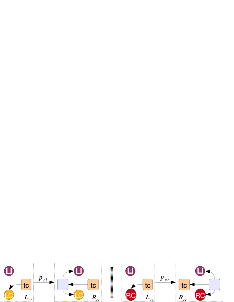
Figure 13: Simulation of an Infinite Tape: Tape Management Productions. $p_{cl}$ Adds a Cell to the Left and $p_{cr}$ Adds a Cell to the Right

Third, the tape of any TM has unbounded capacity. On the MGG side, we want to stick to finite simple digraphs. Two productions (see Fig. 13) will be responsible for tape enlargement just in case it is necessary. The idea is to use the labeled node $LC$ to mark the leftmost cell and $RC$ the rightmost one. Notice however that nodeless MGG does not allow addition nor deletion of nodes.

The point here is that a TM is a uniform model of computation while nodeless MGG is not. There are two possibilities:

• We just need to add nodes. Deletion of nodes is not necessary for TMs. Therefore we may keep the main property of nodeless MGGs (no compatibility issues) if we allow the grammar to add nodes to the tape.

• We may use a non-uniform model of computation and have one nodeless MGG per number of nodes. The only problem with non-uniformity is that various nodeless MGG may have completely dissimilar structure. Precisely, this is avoided with productions $p_{cl}$ and $p_{cr}$. Observe also that addition of nodes have been used just to simulate the infinite tape, but not for modeling the behavior of the TM.

The rest of the section is devoted to an example that models a copy subroutine, taken from [25]. Its behavior is summarized in table 3. This TM replicates any sequence of ones inserting a zero in the middle (the head should be positioned in any of the 1’s that make up the string). For example, it transforms $0000\mathbf{11}0\longmapsto 0110\mathbf{11}0$.

equiv prod		init state	tape symbol	print op	head motion	final state
$p_{10}$		$s_{1}$	0	Nop	Nmov	H
$p_{11}$		$s_{1}$	1	P0	HL	$s_{2}$
$p_{20}$		$s_{2}$	0	P0	HL	$s_{3}$
$p_{21}$		$s_{2}$	1	P1	HL	$s_{2}$
$p_{30}$		$s_{3}$	0	P1	HR	$s_{4}$
$p_{31}$		$s_{3}$	1	P1	HL	$s_{3}$
$p_{40}$		$s_{4}$	0	P0	HR	$s_{5}$
$p_{41}$		$s_{4}$	1	P1	HR	$s_{4}$
$p_{50}$		$s_{5}$	0	P1	HL	$s_{1}$
$p_{51}$		$s_{5}$	1	P1	HR	$s_{5}$
–		H	–	–	–	–

Table 3: Copy Subroutine State Table

In table 3, the first column is the equivalent MGG production, which can be found in Figs. 14 and 15. The rest of the columns specify the TM behavior. Column init state is the initial state of the TM, the third column is the tape symbol in the cell being read, print op is the print operation to be carried out in the tape cell under consideration, head motion indicates where the head should move to and final state is the state assumed by the TM ($H$ is the halting state) which becomes the initial state of the TM for the next operation. For example, the second row ($p_{11}$) says “if your state is $s_{1}$ and there is a 1 (one) in the tape cell, then print a 0 (zero), move to the cell on your left and assume state $s_{2}$”.

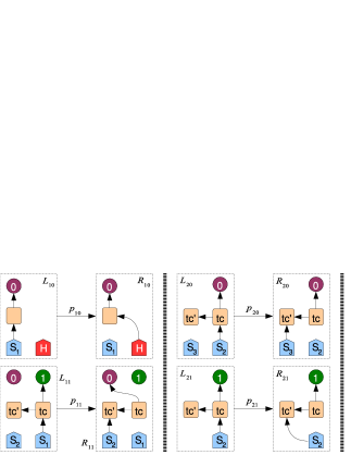
Figure 14: First Six MGG Productions for TM Simulation. Refer to Table 3 for Their TM Counterparts

One production simulates each action of the TM. There are ten, drawn in Figs. 14 and 15. A brief explanation follows:

• Blue squared nodes represent tape cells. Either a 0 or a 1 have to be written on them. As in this example they can not be blank, they should be initialized to 0 (in $p_{cl}$ and $p_{cr}$ on Fig. 13 we should substitute $\sqcup$ by $0$).

• Node $S_{i}$ stands for the $i$th state. It is also used to mark which cell the head points to.

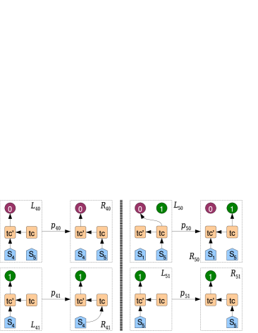
Figure 15: Four More MGG Productions for TM Simulation. Refer to Table 3 for Their TM Counterparts

The set of operations that copies the ones in the word $0\mathbf{11}0$ is $s_{c}=p_{10};p_{50};p_{40};p_{41};\\ p_{30};p_{31};p_{cl};p_{20};p_{11};p_{50};p_{51};p_{40};p_{30};p_{20};p_{cl};p_{21};p_{11}$. This is the sequence that transforms $0\mathbf{11}0$ into $110\mathbf{11}0$. As commented in the introduction, MGG techniques are available for TMs. For example, it is possible to calculate $s_{c}$ – at least we can guess what productions are necessary and the number of times that each one appears – using reachability (see [14] or Chap. 10 in [16]).

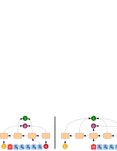
Figure 16: Initial and Final States for the Copy Subroutine

9 MGG and Boolean Circuits

In this section we will simulate Boolean circuits (BC) using nodeless MGG. A standard reference on BCs is [22].

Recall that a BC is a simple digraph. We need only pay attention to the evolution of the circuit, which is equivalent to encoding the representation of the Boolean operations permitted in the BC. In [22], the first thing to do when defining a BC is to fix the Boolean operations allowed. In the present contribution we will restrict ourselves to the Boolean operations and, or and not. The same techniques that will be described apply to any Boolean operation.

There are many ways to encode Boolean operations. We represent the gates with yellow circles labeled with the corresponding Boolean operation. The variables are unlabeled circles in blue. Notice that $x_{i}$ and $y$ are not labels but a means to visually represent which nodes on the LHS are mapped to which nodes on the RHS. On the contrary, $\vee$, $\wedge$, $\neg$, $0$ and $1$ are labels.

Gates labeled with not can only have a single input and a single output node. Gates of types or and and must have two or more inputs and a single output. An unlabeled node is an input variable of some gate if there is an edge from the node to the gate. It will be an output node if there is an edge from the gate to the node. For example, $y$ is an output node in $\neg(0)$ in Fig. 17 and $x$ is an input node.

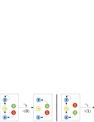
Figure 17: The not Operation

Input and output nodes can be in three states: either no value has been assigned yet (which will be indicated by a self-loop) or it has value $0$ or value $1$ (represented with an edge from a properly labeled node). See Figs. 17, 18 and 19 for some examples.

The not operation (see Fig. 17) is almost self-explanatory. It is not mandatory to delete the input and output edges (to the not node) as the rule would not be applicable to the same elements in the host graph because of the missing self-loop in node $y$. We do it as a visual aid. The value of the input variable is kept (the edge is not deleted) because this node could well be the input of another gate.

We will not limit the number of input nodes to or and and gates. To ease operations, we will demand an ordering in their input nodes. One way to achieve this is to introduce a node se (start-end) to mark the first input node and the last input node for some gate $B$ (= and, or). Every gate of type and and or will have an edge incident to se (each gate $B$ has its own ordering, but a single node may belong to the input nodes of several gates). One edge from input node $x_{1}$ to input node $x_{2}$ will mean that $x_{1}$ goes before $x_{2}$ considered as an input node for gate $B$. See Figs. 18 and 19 for some examples.

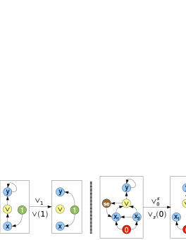
Figure 18: The or Operation

The or operation is represented in Fig. 18. Production $\vee(1)$ forces the result to be $1$ as soon as any input node has this value. Grammar rule $\vee_{s}(0)$ decreases the number of input nodes if both are zero. Notice that $\vee_{s}(0)$ is applied in strict order in the input nodes. Rule $\vee_{e}(0)$ assigns a $0$ to the output gate when only the starting and the ending input nodes are left.

As in the not gate, values assigned to the input nodes are not removed because a single node can be an input for several gates. The same remark applies to the and operation, which is described next.

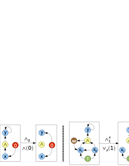
Figure 19: The and Operation

The productions that encode the and operation are depicted in Fig. 19. Their interpretation is very similar to that of the or operation.

The productions that appear in Figs. 17, 18 and 19 simulate Boolean circuits non-deterministically. This non-determinism guarantees that the operations are performed optimally: only those nodes necessary to evaluate the BC will be calculated and in the precise order.

The complexity of a BC is measured in terms of the size (number of gates) and the depth (length of the longest directed path). There are theorems that relate lower bounds on BCs with lower bounds on TMs (see [22]). The non-deterministic encoding of BCs given in this section should not affect this complexity measures. Nevertheless, it should be clear how to transform non-determinism into determinism using some control nodes.

10 Conclusions and Future Work

In the present contribution we have introduced MGG as a formal grammar as well as a model of computation. We have also seen that non-determinism in MGG can be approached through so-called relabeling. It has also been proved that nodeless MGG is capable of simulating deterministic and non-deterministic Turing machines and Boolean Circuits. As a side effect, all MGG techniques are at our disposal to tackle different problems in Turing machines and Boolean Circuits. As commented in Sec. 1, we can (partially) address coherence, congruence, initial state characterization, sequential independence, reachability and some others. Something similar but for Petri nets is done in [14] or in [16], Chap. 10. However, we have not gone into these topics in depth. The theory developed so far can be applied straightforwardly in some cases, while in others some further research is needed.

The use of MGG opens the door to the introduction of analytical and algebraic techniques over finite fields. We are particularly interested in representation theory and abstract harmonic analysis.

Apparently, reachability and the state equation appear to be helpful concepts to address complexity problems. In [14], the reason why the state equation is a necessary but not a sufficient condition is pointed out. It seems natural to move from linear algebra (state equation) to linear programming (positivity restrictions on variables).

Acknowledgements. I would like to express my gratitude to the open source and copyleft communities, in particular to the people behind the text “editor” Emacs (http://www.gnu.org/software/emacs/), TeX Live (the Linux LaTeXdistribution, http://www.tug.org/texlive/), OpenOffice (http://www.openoffice.org) and Linux (http://www.linux.org/), especially the Ubuntu distro (http://www.ubuntu.com/).

References

- [1] Braket notation intro: http://en.wikipedia.org/wiki/Bra-ket_notation
- [2] Baader, F., Nipkow, T. 1999. Term Rewriting and All That. Cambridge University Press. ISBN 0-521-77920-0.
- [3] van Deursen, A., Klint, P., Visser, J. 1999. Domain-Specific Languages: an Annotated Bibliography. http://homepages.cwi.nl/~arie/papers/dslbib/
- [4] Ehrig, H., Ehrig, K., Prange, U., Taentzer, G. 2006. Fundamentals of Algebraic Graph Transformation. Springer.
- [5] Fine, N. J. 1947. Binomial Coefficients Modulo a Prime. Amer. Math. Monthly 54, pp. 589-592.
- [6] Garey, M., Johnson, D. 1979. Computers and Intractability: A Guide to the Theory of NP-Completeness. W.H. Freeman and Company.
- [7] Hopcroft, J., Ullman, J. Introduction to Automata Theory Languages and Computation. 2nd edition. Addison-Wesley Publishing Company, 2000.
- [8] de Lara, J., Vangheluwe, H. 2004. Defining Visual Notations and Their Manipulation Through Meta-Modelling and Graph Transformation. Journal of Visual Languages and Computing. Special section on “Domain-Specific Modeling with Visual Languages”, Vol 15(3-4), pp.: 309-330. Elsevier Science.
- [9] Mètivier, Y., Mosbah, M. 2006. Workshop on Graph Computation Models. LNCS 4178. Springer-Verlag. Berlin. Heidelberg.
- [10] Mosbah, M., Habel, A. 2008. Workshop on Graph Computation Models. LNCS 5214. Springer-Verlag. Berlin. Heidelberg.
- [11] Mulmuley, K., Sohoni, M. A. 2001. Geometric Complexity Theory I: An Approach to the P vs. NP and Related Problems. SIAM J. Comput. 31(2): 496-526.
- [12] Pérez Velasco, P. P., de Lara, J. 2006. Towards a New Algebraic Approach to Graph Transformation: Long Version. Tech. Rep. of the School of Comp. Sci., Univ. Autónoma Madrid. http://www.ii.uam.es/jlara/investigacion/techrep_03_06.pdf.
- [13] Pérez Velasco, P. P., de Lara, J. 2006. Matrix Approach to Graph Transformation: Matching and Sequences. LNCS 4178, pp.:122-137. Springer.
- [14] Pérez Velasco, P. P., de Lara, J. 2006. Petri Nets and Matrix Graph Grammars: Reachability. EC-EAAST(2).
- [15] Pérez Velasco, P. P., de Lara, J. 2007. Using Matrix Graph Grammars for the Analysis of Behavioural Specifications: Sequential and Parallel Independence. ENTCS 206, pp.:133-152. Elsevier.
- [16] Pérez Velasco, P. P. 2009. Matrix Graph Grammars. VDM Verlag e.K. ISBN 978-3-639-21255-6. Also available at: http://www.mat2gra.info/, CoRR abs/0801.1245.
- [17] Pérez Velasco, P. P., de Lara, J. 2009. Matrix Graph Grammars and Monotone Complex Logics. Available at: http://www.mat2gra.info/, CoRR abs/arXiv:0902.0850v1.
- [18] Pérez Velasco, P. P., de Lara, J. 2009. A Reformulation of Matrix Graph Grammars with Boolean Complexes. The Electronic Journal of Combinatorics. Vol. 16(1). R73. Available at: http://www.combinatorics.org/
- [19] Pérez Velasco, P. P., de Lara, J. 2010. Matrix Graph Grammars with Application Conditions. To appear in Fundamenta Informaticae. IOS Press.
- [20] Rozenberg, G. (managing Ed.) 1999. Handbook of Graph Grammars and Computing by Graph Transformation. Vol.1 (Foundations), Vol.2 (Applications, Languages and Tools), Vol.3 (Concurrency, Parallelism and Distribution). World Scientific.
- [21] Sipser, M. 1996. Introduction to the Theory of Computation. PWS Pub. Co. ISBN 978-0534947286.
- [22] Vollmer, H. 1999. Introduction to Circuit Complexity. A Uniform Approach. Springer. ISBN 978-3540643104.
- [23] Weisstein, E. Sierpiński Sieve. “From MathWorld–A Wolfram Web Resource”. http://mathworld.wolfram.com/SierpinskiSieve.html
- [24] Weisstein, E. Permutation Matrix. “From MathWorld–A Wolfram Web Resource”. http://mathworld.wolfram.com/PermutationMatrix.html
- [25] Wikipedia Contributors, 2007. Turing Machines Examples. Wikipedia, The Free Encyclopedia. http://en.wikipedia.org/w/index.php?title=Turing˙machine˙examples&oldid=17499887