Luminescence of a Cooper Pair

Abstract

This paper theoretically discusses the photon emission spectra of a superconducting pn-junction. On the basis of the second order perturbation theory for electron-photon interaction, we show that the recombination of a Cooper with two p-type carriers causes drastic enhancement of the luminescence intensity. The calculated results of photon emission spectra explain characteristic features of observed signal in an recent experiment. Our results indicate high functionalities of superconducting light-emitting devices.

Light-emitting diode (LED) usually fabricated on semiconductors has been an important element of modern technologies. A trend of research seems to be focusing on producing a better controlled photon and an entangled photon pair michler ; benson for realizing quantum computation and quantum information. Superconducting devices have an advantage to obtain robustly coherent quantum states because of its coherent nature chiorescu ; wallraff ; katz . Superconducting LEDs hanamura have been originally proposed in the context of superradiation. They are, however, a promising candidate to create an entangled photon pair suemune . A recent theoretical study predicts the Josephson radiation in a superconducting pn junction recher . Thus superconductor/semiconductor LED hybrids undoubtedly have a possibility to produce technologies in the next generation.

The radiative recombination of Cooper pairs has been observed recently in a InGaAs/InP pn junction attaching onto a superconductor Nb hayashi . The electroluminescence becomes drastically large at low temperatures below the superconducting transition temperature $T_{c}$ of Nb electrode. Surprisingly degree of the enhancement in the luminescence intensity is one order of magnitude. Although the effects of superconductivity on the radiative recombination are clear in experiments, a mechanism has been an open problem. We theoretically address this issue in this paper. We study the emission spectra of photon in a superconducting pn junction based on the second order perturbation theory. In the second order expansion, we find that a peculiar recombination process to superconductivity enlarges the luminescence intensity, where two electrons recombine with two p-type carriers as a Cooper. The theoretical results explain characteristic features of the experimental findings hayashi . This paper not only figures out a mechanism of the large amplitude of luminescence intensity but also gives a guide for designing highly functional superconducting light-emitting devices.

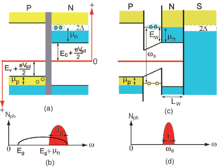
Figure 1: (Color online) Schematic energy diagram of pn junctions. A theoretical model used for calculation is shown in (a). In (c), a real junction in an experiment is illustrated. Theoretical results of the photon spectra are shown in (b) and (d).

Let us consider a p-type semiconductor / superconductor junction as shown in Fig. 1(a). The energy is measured from the horizontal line indicated by ’0’. The sign of energy in a p-type semiconductor is chosen to be opposite to that in a superconductor. We assume that a semiconductor and a superconductor are in their local equilibrium which are characterized by the local chemical potential $\mu_{p}$ and $\mu_{n}$, respectively. The edges of the conduction and valence bands are $E_{c}$ and $E_{v}$, respectively. In what follows, we use a unit of $\hbar=k_{B}=c=1$, where $k_{B}$ is the Boltzmann constant and $c$ is the speed of light. The p-type semiconductor is described by

$$H_{p}=\sum_{\boldsymbol{k},\sigma}\epsilon_{p}(k)b_{\boldsymbol{k},\sigma}^{\dagger}b_{\boldsymbol{k},\sigma},$$ (1)

where $\epsilon_{p}(k)={k}^{2}/(2m_{p})+E_{v}+eV_{sd}/2$, $m_{p}$ is the effective mass, $V_{sd}$ is the applied bias voltage across the junction, and $b_{\boldsymbol{k},\sigma}^{\dagger}(b_{\boldsymbol{k},\sigma})$ is the creation (annihilation) operator of a p-type carrier with a wave number $\boldsymbol{k}$ and spin $\sigma=\uparrow$ or $\downarrow$. The photon states is described by

$$H_{ph}= \sum_{\boldsymbol{q}}\omega_{q}\left(a_{\boldsymbol{q}}^{\dagger}a_{\boldsymbol{q}}+\frac{1}{2}\right),$$ (2)

where $a_{\boldsymbol{q}}^{\dagger}(a_{\boldsymbol{q}})$ is the creation (annihilation) operator of a photon with a wave number $\boldsymbol{q}$ and an energy $\omega_{q}$. The normal state in a metal is described by

$$H_{nn}= \sum_{\boldsymbol{k},\sigma}\left(\frac{k^{2}}{2m_{n}}+E_{c}+\frac{eV_{sd}}{2}\right)c_{\boldsymbol{k},\sigma}^{\dagger}c_{\boldsymbol{k},\sigma},$$ (3)

with $m_{n}$ being the effective mass. The electron-photon interaction Hamiltonian reads

$$H_{I}=\sum_{\boldsymbol{k},\boldsymbol{q},\sigma}B_{\boldsymbol{k},\boldsymbol{q}}\,b_{\boldsymbol{k}-\boldsymbol{q},\sigma}\,\,c_{\boldsymbol{k},\sigma}\,a_{\boldsymbol{q}}^{\dagger}+\text{H.c.},$$ (4)

where $B_{\boldsymbol{k},\boldsymbol{q}}$ is the coupling energy. On the basis of the second order perturbation theory, the number of photon $N_{ph}=\sum_{\boldsymbol{q}}a_{\boldsymbol{q}}^{\dagger}a_{\boldsymbol{q}}$ is calculated as

$$\langle N_{ph}\rangle=\langle N_{ph}(1)\rangle+\langle N_{ph}(2)\rangle,$$ (5)

$$\langle N_{ph}(1)\rangle=\int_{-\infty}^{t}\!\!\!\!\!dt_{1}\int_{-\infty}^{t}\!\!\!\!\!dt_{2}\langle\chi_{0}|H_{I}(t_{1})N_{ph}H_{I}(t_{2})|\chi_{0}\rangle,$$ (6)

$$\langle N_{ph}(2)\rangle=\int_{-\infty}^{t_{2}}\!\!\!\!\!dt_{1}\int_{-\infty}^{t}\!\!\!\!\!dt_{2}\int_{-\infty}^{t}\!\!\!\!\!dt_{3}\int_{-\infty}^{t_{3}}\!\!\!\!\!dt_{4}\;I(2),$$ (7)

$$I(2)=\langle\chi_{0}|H_{I}(t_{1})H_{I}(t_{2})N_{ph}H_{I}(t_{3})H_{I}(t_{4})|\chi_{0}\rangle,$$ (8)

$$|\chi_{0}\rangle\to|0\rangle\otimes|N\rangle\otimes|P\rangle,$$ (9)

where $|0\rangle$ is the zero photon state.

The BCS theory describes superconducting states,

$$H_{ns}= \sum_{\boldsymbol{k},\sigma}E_{k}\gamma_{\boldsymbol{k},\sigma}^{\dagger}\gamma_{\boldsymbol{k},\sigma},$$ (10)

where $E_{k}=\sqrt{\xi_{n}^{2}(k)+\Delta^{2}}$, $\xi_{n}(k)={k^{2}}/{2m_{n}}-\mu_{n}$, $\Delta$ is the pair potential, and $\gamma_{\boldsymbol{k},\sigma}^{\dagger}(\gamma_{\boldsymbol{k},\sigma})$ is the creation (annihilation) operator of Bogoliubov quasiparticle. This description, however, is valid within a small energy scale near the Fermi level which is at $\tilde{\mu}_{n}=E_{c}+eV_{sd}/2+\mu_{n}$ measured from ’0’. To apply the BCS theory to the present issue, a rule is necessary to describe the operator in the interaction picture. The canonical transformation connects an electron operator and Bogoliubov operators by

$$c^{\dagger}_{\boldsymbol{k},\sigma}(t)=e^{i\tilde{\mu}_{n}t}\left(u_{k}e^{iE_{k}t}\gamma_{\boldsymbol{k},\sigma}^{\dagger}\ -s_{\sigma}v_{k}e^{-iE_{k}t}\gamma_{-\boldsymbol{k},\bar{\sigma}}\right),$$ (11)

in $\langle\chi_{0}|\cdots|\chi_{0}\rangle$, where $u_{k}(v_{k})=[(1+(-)\xi_{n}(k)/E_{k})/2]^{1/2}$, $s_{\sigma}=1(-1)$ for $\sigma=\uparrow(\downarrow)$, and $\bar{\sigma}$ means the opposite spin to $\sigma$. The thermal average of operators is carried out in the local equilibrium. In a p-type semiconductor, for instance, the average of operators are calculated in

$$H_{p}^{\prime}=\sum_{\boldsymbol{k},\sigma}\xi_{p}(k)b_{\boldsymbol{k},\sigma}^{\dagger}b_{\boldsymbol{k},\sigma},$$ (12)

instead of Eq. (1) with $\xi_{p}(k)=k^{2}/2m_{p}-\mu_{p}$. In a superconductor, the average of the Bogoliubov operators are calculated in Eq. (10). In Eq. (9), $|P\rangle$ means the state vector of p-type carrier in the local equilibrium and $|N\rangle$ indicates the BCS state in the local equilibrium.

The time average of the photon number $\overline{\langle N_{ph}\rangle}$ corresponds to the luminescence intensity and it in the first order perturbation expansion results in

$$\overline{\langle N_{ph}(1)\rangle}=2\pi\sum_{\boldsymbol{k},\boldsymbol{q},\sigma}|B_{\boldsymbol{k},\boldsymbol{q}}|^{2}f^{p}_{\boldsymbol{k}-\boldsymbol{q}}$$

$$\times\left[u_{k}^{2}f^{n}_{k}\delta(\tilde{\omega}-E_{k})+v_{k}^{2}(1-f^{n}_{k})\delta(\tilde{\omega}+E_{k})\right],$$ (13)

where $\tilde{\omega}=\omega_{q}-E_{g}-\mu_{n}-\mu_{p}-\xi_{p}(\boldsymbol{k}-\boldsymbol{q})$, $E_{g}=E_{v}+E_{c}+eV_{sd}$, $f^{n}_{k}=[1-\tanh(E_{k}/2T)]/2$, and $f^{p}_{k}=[1-\tanh(\xi_{p}(k)/2T)]/2$. This result recovers the photon spectra in a normal pn junction by tuning $\Delta\to 0$, which means that $E_{k}\to-\xi_{n}(k),u_{k}\to 0$, $v_{k}\to 1$ for $k<k_{F}$ and $E_{k}\to\xi_{n}(k),u_{k}\to 1$, $v_{k}\to 0$ for $k>k_{F}$ with $k_{F}$ being the Fermi wave number satisfying $k_{F}^{2}/2m_{n}=\mu_{n}$. The threshold of spectra is $E_{g}$ and the width of spectra is given by $\mu_{n}+\mu_{p}$. The spectra in Eq. (13) have a broad profile reflecting the quasiparticle density of states as shown in Fig. 1(b).

One of the characteristics peculiar to superconductivity is a giant oscillator strength hanamura . This comes from the much freedom of the wave vector $\boldsymbol{k}$ for the remaining elementary excitation when a Cooper pair decays radiatively with a p-type carrier with the opposite wave vector $-\boldsymbol{k}$. This would gives the large luminescence intensity in the experiment hayashi . This effect of the giant oscillator strength works also in the first stage in the second order expansion while not in the second process. The other characteristics is coming from the resonant enhancement due to the nearly degenerate nature of the final and intermediate states close to the initial state. This is shown in the following calculation.

The results of the second order perturbation are given by

$$I(2)= \!\!\!\!\!\!\sum_{\boldsymbol{k}_{1}\cdots\boldsymbol{k}_{4},\boldsymbol{q}_{1}\cdots\boldsymbol{q}_{4},\sigma_{1}\cdots\sigma_{4}}\!\!\!\!\!\!\!\!\!\!\!\!\!\!\!\!\!\!e^{-i\Omega_{1}t_{1}-i\Omega_{2}t_{2}+i\Omega_{3}t_{3}+i\Omega_{4}t_{4}}$$

$$\times B^{\ast}_{\boldsymbol{k}_{1},\boldsymbol{q}_{1}}B^{\ast}_{\boldsymbol{k}_{2},\boldsymbol{q}_{2}}B_{\boldsymbol{k}_{3},\boldsymbol{q}_{3}}B_{\boldsymbol{k}_{4},\boldsymbol{q}_{4}}Q_{Ph}Q_{P}Q_{N},$$ (14)

with $\Omega_{j}(\boldsymbol{k}_{j},\boldsymbol{q}_{j})=\omega_{q_{j}}-\epsilon_{P}(\boldsymbol{k}_{j}-\boldsymbol{q}_{j})-\tilde{\mu}_{n}$. The average of the operators $Q_{Ph}$, $Q_{P}$ and $Q_{N}$ are calculated as follows,

$$Q_{Ph}= \sum_{\boldsymbol{q}_{5}}\langle 0|a_{\boldsymbol{q}_{1}}a_{\boldsymbol{q}_{2}}a_{\boldsymbol{q}_{5}}^{\dagger}a_{\boldsymbol{q}_{5}}a_{\boldsymbol{q}_{3}}^{\dagger}a_{\boldsymbol{q}_{4}}^{\dagger}|0\rangle,$$

$$= 2(\delta^{\boldsymbol{q}}_{14}\delta^{\boldsymbol{q}}_{23}+\delta^{\boldsymbol{q}}_{13}\delta^{\boldsymbol{q}}_{24}),$$ (15)

$$Q_{P}= \langle P|b^{\dagger}_{\boldsymbol{p}_{1},\sigma_{1}}b^{\dagger}_{\boldsymbol{p}_{2},\sigma_{2}}b_{\boldsymbol{p}_{3},\sigma_{3}}b_{\boldsymbol{p}_{4},\sigma_{4}}|P\rangle,$$

$$= f_{\boldsymbol{p}_{1}}^{p}f_{\boldsymbol{p}_{2}}^{p}(\delta^{\sigma}_{14}\delta^{\sigma}_{23}\delta^{\boldsymbol{p}}_{14}\delta^{\boldsymbol{p}}_{23}-\delta^{\sigma}_{13}\delta^{\sigma}_{24}\delta^{\boldsymbol{p}}_{13}\delta^{\boldsymbol{p}}_{24}),$$ (16)

where $\delta^{\boldsymbol{q}}_{ij}=\delta_{\boldsymbol{q}_{i},\boldsymbol{q}_{j}}$, $\delta^{\sigma}_{ij}=\delta_{\sigma_{i},\sigma_{j}}$, $\delta^{\boldsymbol{p}}_{ij}=\delta_{\boldsymbol{p}_{i},\boldsymbol{p}_{j}}$ and $\boldsymbol{p}_{j}=\boldsymbol{k}_{j}-\boldsymbol{q}_{j}$. By applying the Bogoliubov transformation, we find,

$$Q_{N}=\langle N|(u_{k_{1}}e^{iE_{k_{1}}t_{1}}\gamma_{\boldsymbol{k}_{1},\sigma_{1}}^{\dagger}-\sigma_{1}v_{k_{1}}e^{-iE_{k_{1}}t_{1}}\gamma_{-\boldsymbol{k}_{1},\bar{\sigma}_{1}})$$

$$\times(u_{k_{2}}e^{iE_{k_{2}}t_{2}}\gamma_{\boldsymbol{k}_{2},\sigma_{2}}^{\dagger}-\sigma_{2}v_{k_{2}}e^{-iE_{k_{2}}t_{2}}\gamma_{-\boldsymbol{k}_{2},\bar{\sigma}_{2}})$$

$$\times(u_{k_{3}}e^{-iE_{k_{3}}t_{3}}\gamma_{\boldsymbol{k}_{3},\sigma_{3}}-\sigma_{3}v_{k_{3}}e^{iE_{k_{3}}t_{3}}\gamma_{-\boldsymbol{k}_{3},\bar{\sigma}_{3}}^{\dagger})$$

$$\times(u_{k_{4}}e^{-iE_{k_{4}}t_{4}}\gamma_{\boldsymbol{k}_{4},\sigma_{4}}-\sigma_{4}v_{k_{4}}e^{iE_{k_{4}}t_{4}}\gamma_{-\boldsymbol{k}_{4},\bar{\sigma}_{4}}^{\dagger})|N\rangle,$$ (17)

which gives twelve terms. In what follows, we extract the most dominant contribution in the second order terms. The average of $Q_{N}$ includes following four terms

$$Q_{N} (S)=u_{k_{1}}v_{k_{1}}u_{k_{3}}v_{k_{3}}\delta_{\sigma_{1},\bar{\sigma}_{2}}\delta_{\sigma_{3},\bar{\sigma}_{4}}\delta_{\boldsymbol{k}_{1},-\boldsymbol{k}_{2}}\delta_{\boldsymbol{k}_{3},-\boldsymbol{k}_{4}}\sigma_{1}\sigma_{3}$$

$$\times\left[e^{iE_{k_{1}}(t_{1}-t_{2})}e^{-iE_{k_{3}}(t_{3}-t_{4})}f^{n}_{k_{1}}(1-f^{n}_{k_{3}})\right.$$

$$+e^{-iE_{k_{1}}(t_{1}-t_{2})}e^{iE_{k_{3}}(t_{3}-t_{4})}f^{n}_{k_{3}}(1-f^{n}_{k_{1}})$$

$$-e^{-iE_{k_{1}}(t_{1}-t_{2})}e^{-iE_{k_{3}}(t_{3}-t_{4})}(1-f^{n}_{k_{1}})(1-f^{n}_{k_{3}})$$

$$\left.-e^{iE_{k_{1}}(t_{1}-t_{2})}e^{iE_{k_{3}}(t_{3}-t_{4})}f^{n}_{k_{1}}f^{n}_{k_{3}}\right].$$ (18)

Because $\delta_{\sigma_{3},\bar{\sigma}_{4}}\delta_{\boldsymbol{k}_{3},-\boldsymbol{k}_{4}}$ in Eq. (18) means the destruction of two electrons as a Cooper pair, $Q_{N}(S)$ describe effects of superconductivity on the emission spectra. Another eight terms in $Q_{N}$ contribute to the emitting processes described by Fig. 2(b) which gives the luminescence intensity proportional to $\overline{\langle N_{ph}(1)}\rangle^{2}$. We will show that $Q_{N}(S)$ gives a large contribution to the emission spectra at $\delta\boldsymbol{q}=\boldsymbol{q}_{1}+\boldsymbol{q}_{2}=0$, ($\delta\boldsymbol{q}=\boldsymbol{q}_{3}+\boldsymbol{q}_{4}=0$ in other wards) smallq . Substituting Eqs. (15),(16) and (18) into Eq. (14) and carrying out time integrations, we obtain

$$\overline{\langle N_{ph}(2)\rangle}= 4\pi|B|^{4}\sum_{\boldsymbol{q},\sigma}\delta(\Omega_{\boldsymbol{k}_{F},\boldsymbol{q}})I_{0},$$ (19)

$$I_{0}= \sum_{\boldsymbol{k}}\left[\frac{f^{n}_{k}(1-f^{n}_{k})}{(E_{k}-i/\tau)^{2}}+\frac{f^{n}_{k}(1-f^{n}_{k})}{(E_{k}+i/\tau)^{2}}\right.$$

$$\left.+\frac{(f^{n}_{k})^{2}+(1-f^{n}_{k})^{2}}{E_{k}^{2}+(1/\tau)^{2}}\right]\frac{\Delta^{2}}{E_{k}^{2}},$$ (20)

where we introduce a relaxation time $\tau$ to remove effects of the perturbation at $t\to-\infty$, we neglect dependence of $B$ on wave numbers and assume $f^{p}_{\boldsymbol{k}_{F}-\boldsymbol{q}}=1$. At $1/\tau=0$, $I_{0}=\pi N_{0}/2\Delta$ essentially diverges for small $\Delta$ with $N_{0}$ denoting the normal density of states in a superconductor at the Fermi energy. The singular behavior at small $\Delta$ in Eq. (20) is a sign of the large luminescence intensity due to superconductivity.

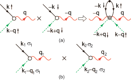
Figure 2: (Color online) Recombination processes in the second order perturbation expansion, where solid, broken and wavy lines represent the propagation of an electron, a p-type carrier and a photon, respectively In (a), a recombination of a Cooper pair in $Q_{N}(S)$ is shown. In (b), a recombination process other than $Q_{N}(S)$ is illustrated.

We first show mathematical reasons of the singularity. Then we will discuss the physics behind the phenomenon. A two-photon emitting process in $Q_{N}(S)$ is illustrated in Fig. 2(a). The annihilation of a Cooper pair is described by $c_{-\boldsymbol{k},\downarrow}c_{\boldsymbol{k},\uparrow}$ which includes a operator $\gamma_{\boldsymbol{k},\uparrow}^{\dagger}\gamma_{\boldsymbol{k},\uparrow}$. Let us assume that the energy of the initial state is zero. In the first order expansion, the operation of $\gamma_{\boldsymbol{k},\uparrow}$ to the BSC state decreases energy by $E_{k}+\tilde{\mu}_{n}$. At the same time, a p-type carrier with energy $\epsilon_{p}(\boldsymbol{k}-\boldsymbol{q})$ is destructed and a photon with energy $\omega_{q}$ is created. Thus the energy of the intermediate state $\delta E_{1}$ results in $\delta E_{1}=\omega_{q}-\epsilon_{p}(\boldsymbol{k}-\boldsymbol{q})-E_{k}-\tilde{\mu}_{n}=\Omega_{\boldsymbol{k},\boldsymbol{q}}-E_{k}$ which is the energy denominator in the perturbation expansion. In the second order, the operation of $\gamma_{\boldsymbol{k},\uparrow}^{\dagger}$, the destruction of a p-type carrier, and the creation of a photon gain energy by $E_{k}-\tilde{\mu}_{n}$, $-\epsilon_{p}(-\boldsymbol{k}+\boldsymbol{q})$, and $\omega_{-q}$, respectively. Therefore the difference in energy between the intermediate state and the final one becomes $\delta E_{2}=\omega_{q}-\epsilon_{p}(\boldsymbol{k}-\boldsymbol{q})+E_{k}-\tilde{\mu}_{n}=\Omega_{\boldsymbol{k},\boldsymbol{q}}+E_{k}$. The perturbation theory requires the energy conservation between the initial and the final states, (i.e., $\delta E_{1}+\delta E_{2}=0$), which leads to $2\Omega_{\boldsymbol{k},\boldsymbol{q}}=0$. As a result, only a small value of $E_{k}$ remains in the denominator as shown in Eq. (20). The physics behind the phenomena is simple. The BCS state can have ability to emit a pair of photons with remaining its state almost unchanged because the BCS state is the eigen state of $\gamma_{\boldsymbol{k},\uparrow}^{\dagger}\gamma_{\boldsymbol{k},\uparrow}$. The equation $\Omega_{\boldsymbol{k}_{F},\boldsymbol{q}}=0$ is the condition for emitting a photon. The threshold and width of spectra are $E_{g}+\mu_{n}$ and $\mu_{p}$, respectively. In Fig. 1(b), we show predicted spectra in the second order process.

The singular behavior in perturbation expansion implies an importance of higher order terms to predict the luminescence intensity quantitatively. Here we do not discuss this issue, but choose an alternative way of regularizing the obtained results for qualitative argument. In what follows, we introduce a finite relaxation time. First we consider mean free time due to elastic impurity scatterings $\tau_{0}$. At $T=0$, we obtain $I_{0}=I_{00}(0)2\alpha^{2}/(\sqrt{1+\alpha^{2}}(\alpha+\sqrt{1+\alpha^{2}}))$, where $\alpha=\tau_{0}\Delta_{0}$, $\Delta_{0}$ is the pair potential at the zero temperature and $I_{00}(0)=\pi N_{0}/2\Delta_{0}$ is Eq. (20) at $T=0$. At $T\lesssim T_{c}$, we find

$$\frac{I_{0}}{I_{00}(0)}\approx\left\{\begin{array}[]{ll}c_{0}\alpha^{2}(\Delta/\Delta_{0})^{2}\Delta_{0}/T&\alpha\lesssim 1\\ \alpha^{3}(\Delta/\Delta_{0})^{2}&\alpha\gg 1,\end{array}\right.$$ (23)

where $c_{0}$ is a constant of the order of unity. In Fig. 3(a), we show $I_{0}$ as a function of temperature for several choices of $\alpha$, where we describe the dependence of $\Delta$ on temperature by the BCS theory. The amplitude of $I_{0}$ at $T=0$ is suppressed in the dirty limit as shown in a result with $\alpha=0.2$. The amplitude at $T=0$ increases with increasing $\alpha$. At $\alpha=1$, $I_{0}(0)$ has almost the same amplitude as $I_{00}(0)$. When we increase $\alpha$ up to 2.0, the results show a bump just below $T_{c}$. Next we consider inelastic scatterings described by $1/{\tau_{ie}}=C_{ie}\left({T}/{T_{c}}\right)^{p}$, where $C_{ie}$ is a coupling constant and $p$ depends on scattering sources such as $p=1$ for electron-phonon scatterings and $p=2$ for repulsive electron-electron interaction. In Fig. 3(b), we calculate $I_{0}$ for several choices of $C_{ie}$ and $p$. Since $1/\tau_{ie}\to 0$ at $T=0$, the amplitude is close to $I_{00}(0)$ at $T=0$. When we decreases $C_{ie}$, the bump appears below $T_{c}$ as well as in (a). For $1/\tau\lesssim\Delta_{0}$, the luminescence intensity at $T\lesssim T_{c}$ is then given by

$$\overline{\langle N_{ph}(2)\rangle} \approx 4\pi c_{0}|B|^{4}N_{0}\frac{(\tau\Delta)^{2}}{T}\sum_{q}\delta(\Omega_{k_{F},q}).$$ (24)

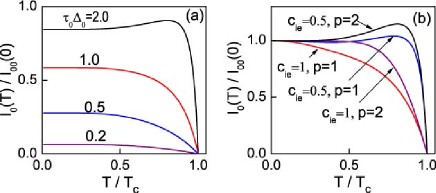
Figure 3: Temperature dependence of luminescence intensity. In (a), we consider relaxation time due to the elastic impurity scatterings by $\alpha=\tau_{0}\Delta_{0}$. In (b), we consider the relaxation due to inelastic scatterings.

Finally we modify Eq. (24) to describe the photon spectra in the experiment hayashi as shown in Fig. 1(c). In the real junction, a superconductor is attached to a n-type semiconductor whose thickness is $L_{w}$. The proximity effect enhances the luminescence intensity. In Eq. (24), $\Delta$ is proportional to the amplitude of a Cooper pair. In n-type semiconductor, the proximity effect enables the pair amplitude which proportional to $\Delta e^{-L_{w}/\xi_{T}}$ with $\xi_{T}=\sqrt{D/2\pi T}$ and $D$ being the diffusion constant in the n-type semiconductor. The photon pairs are emitted in a quantum well between the p- and n-type semiconductors. The level in the quantum well $E_{w}$ should coincide with the Fermi level in the n-type semiconductor $\mu_{n}$. Namely $|E_{w}-\mu_{n}|$ must be less than both the Thouless energy $E_{Th}=D/L_{w}^{2}$ and $\Delta$. This resonant condition is particularly important for a Cooper pair to penetrate into the quantum well. The emission spectra has a peak at $\omega_{0}$ and the peak width is given by $\Gamma=t_{w}^{2}N_{0}$, where $t_{w}$ is the transfer integral between the quantum well and the semiconductor. The argument above is summarized by an equation for $T\lesssim T_{c}$

$$\overline{\langle N_{ph}(2)\rangle}\approx|B|^{4}N_{0}\Gamma\sum_{\boldsymbol{q},\sigma}\frac{\Delta^{2}\tau^{2}e^{-2L_{W}/\xi_{T}}/T}{(\omega_{q}-\omega_{0})^{2}+(\Gamma)^{2}},$$ (25)

where we introduce the Lorentz resonant function by hand. In the experiment, $\xi_{T}$ is estimated to be much larger than $L_{w}$ below $T_{c}$. Thus the theoretical results in Fig. 3 can describe experimental results of the luminescence intensity. In fact, the experimental results of Fig. 6(b) in Ref. hayashi, show a very similar line shape to that in Fig. 3(a) with $\alpha=1$.

In conclusion, we have studied the photon emission spectra in a superconducting pn junction based on the second order perturbation theory for electron-photon interaction. We have found in the second order expansion that a peculiar recombination process to superconductivity enlarges the luminescence intensity. The theoretical results explain temperature dependence of the luminescence intensity observed in an recent experiment.

References

(1) P. Michler, A. Kiraz, C. Becher, W. V. Schoenfeld,
P. M. Petroff, Lidong Zhang, E. Hu, A. Imamogulu, Science 290, 2282 (2000).
(2) O. Benson, C. Santori, M. Pelton, and Y. Yamamoto,
Phys. Rev. Lett. 84, 2513 (2000).
(3)I. Chiorescu, P. Bertet, K. Semba, Y. Nakamura, C. J. P. M. Harmans, and
J. E. Mooij, Nature 431, 159 (2004).
(4)A. Wallraff, D. I. Schuster, A. Blais, L. Frunzio, R.-S. Huang, J. Majer, S. Kumar,
S. M. Girvin, and R. J. Schoelkopf, Nature 431, 162 (2004).
(5) N. Katz, M. Ansmann, R. C. Bialczak, E. Lucero, R. McDermott, M. Neeley,
M. Steffen, E. M. Weig, A. N. Cleland, J. M. Martinis, and A. N. Korotkov,
Science 312, 1498 (2006).
(6) E. Hanamura, physica stat. solidi b 234, 166 (2002).
(7) I. Suemune, T. Akazaki, K. Tanaka, M. Jo, K. Uesugi, M. Endo, H. Kumano,
E. Hanamura, H. Takayanagi, M. Yamanishi, and H. Kan, Japan. J. Appl. Phys. 45,
9264 (2006).
(8) Y. Hayashi, K. Tanaka, T. Akazaki, M. Jo, H. Kumano, and I. Suemune,
Appl. Phys. Express 1, 011701 (2008).
(9)P. Recher, Y. V. Nazarov, L. Kouwenhoven, arXiv:0902-4468.
(10) The speed of light is much larger than the Fermi velocity.
In such case, this condition becomes .