Enhancement of charged macromolecule capture by nanopores in a salt gradient

Abstract

Nanopores spanning synthetic membranes have been used as key components in proof-of-principle nanofluidic applications, particularly those involving manipulation of biomolecules or sequencing of DNA. The only practical way of manipulating charged macromolecules near nanopores is through a voltage difference applied across the nanopore-spanning membrane. However, recent experiments have shown that salt concentration gradients applied across nanopores can also dramatically enhance charged particle capture from a low concentration reservoir of charged molecules at one end of the nanopore. This puzzling effect has hitherto eluded a physically consistent theoretical explanation. Here, we propose an electrokinetic mechanism of this enhanced capture that relies on the electrostatic potential near the pore mouth. For long pores with diameter much greater than the local screening length, we obtain accurate analytic expressions showing how salt gradients control the local conductivity which can lead to increased local electrostatic potentials and charged analyte capture rates. We also find that the attractive electrostatic potential may be balanced by an outward, repulsive electroosmotic flow (EOF) that can in certain cases conspire with the salt gradient to further enhance the analyte capture rate.

I Introduction

Recent interest in electrokinetic manipulation of charged macromolecules has been motivated by technological applications, particularly those involving sorting and sequencing of nucleic acids. In a typical realization of single molecule DNA sequencing, an ionic solution is separated by a membrane with a small pore across the membrane, connecting two otherwise separated bulk reservoirs (cf. Fig. 1). When an electric potential is applied across the membrane, ionic current flowing through the pore is detected. DNA and protein molecules placed on one side of the membrane (the right reservoir in Fig. 1), even at low concentrations, can occasionally block the pore, reducing the ionic current. A time trace of the ionic current flowing across the pore therefore directly measures the statistics of blocking and unblocking events.

Experimentally, numerous modifications of the basic configuration have been studied. Biological pores such as $\alpha$-hemolysin have also been chemically modified to alter internal charges, leading to possible enhancements of the capture frequency and translocation rates of biopolymers through the pore BAYLEY2008 . A number of groups have also recently fabricated synthetic pores GOLOVCHENKO ; MARZIALI ; DEKKER , typically through SiN membranes, for use in macromolecule capture experiments. Besides pore design, other approaches to better control macromolecular analyte (both charged and uncharged) capture and translocation have been explored. In recent measurements using synthetic pores, an enhanced capture rate of DNA was observed in the presence of a salt gradient MELLERABS ; WANUNUABS . Salt added to the opposing, non-analyte reservoir increased the capture rate as a function of the salt ratio between the two reservoirs.

Much of the theoretical effort, including molecular simulations, has concentrated on the physics of polymer translocation through the pore KLAFTER ; PARK ; SCHULTEN . However, since macromolecular capture is sensitive to applied voltage, occurs even with uncharged molecules, and is a stochastic process, the relevant mechanism will involve the interplay among electrostatics, fluid flow, and the statistics of capture. Although the electric potentials and flows inside a nanopore have been presented in the context of Poisson-Nernst-Planck models EISENBERG1997 ; EISENBERG , the dynamics of initial particle capture requires a more detailed analysis of the field configuration in the bulk reservoir, near the pore opening. Finally, the analyte density in the reservoir needs to be determined GOLOVCHENKO in order to solve the problem of capture of a charged macromolecule to the pore mouth in the presence of fluid flow and electrokinetic forces that stochastically switch according to pore blockage. The polymer capture problem has been treated by Wong and Muthukumar WONGMUTHU , who derive capture rates in the presence of electroosmotic flow (EOF) induced by an applied voltage bias and surface charges on the inner pore surface. In this study, as in many others, WONGMUTHU ; SCHULTEN ; EISENBERG1992 the electric field in the reservoir was neglected and the capture problem was solved only in the fast translocation limit.

In this paper, we show that bulk electric fields and a more detailed calculation of the capture problem are necessary to explain the recently-observed salt gradient-induced enhancement of charged analyte capture rates. By using geometrical approximations in the high salt limit, we find analytic expressions for the local salt concentration and electrostatic potential that are accurate for a range of parameters relevant to typical experiments. In the presence of an imposed salt concentration gradient, we show that although most of the potential drop occurs across thin pores, the electrostatic potential at the pore mouth plays an important role in the analyte capture rate and cannot be neglected. We also show how an EOF into the analyte reservoir (by itself convecting macromolecules away from the pore) can interact nonlinearly with the salt gradient and electrostatic potential to actually increase the capture rate. Finally, we analyze implicit solutions for mean capture rates using the full steady-state Debye-Smulochowski capture problem with a partially absorbing boundary for the analyte concentration at the pore mouth.

II Electrokinetic equations

A typical experimental set-up is depicted in Fig. 1(a) where two reservoirs containing aqueous solution are separated by an electrically insulating membrane containing a single conducting nanopore through which fluid can flow. A voltage bias $v$ is applied across electrodes placed far from the pore, resulting in an ionic current through it.

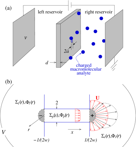
Figure 1: Schematic of electrokinetic focussing experiments. (a) Charged analytes are placed in the right reservoir and a voltage bias is applied. (b) The structure of the pore, electrostatic potential, and electroosmotically driven fluid flow in dimensionless units, with distance measured in units of the pore radius. For long pores ($a/d=w\ll 1$), the concentration and potential fields are approximated as constant within the small hemispherical regions capping the pore (denoted by $\pm$). Field and flux continuity conditions are applied at the hemispherical surfaces. The electroosmotic flow field in the right chamber will be approximately spherically symmetric (red) if the membrane surface is uniformly charged but will be more lobe-like (black) if the membrane flange is uncharged and no-slip boundary conditions are imposed WEINBAUM ; PARMET .

The full steady-state electrokinetic equations for the local electrostatic potential $\Phi({\bf r},t)$, ion concentration $C_{i}({\bf r},t)$, and local fluid velocity ${\bf U}({\bf r},t)$:

$$\nabla\cdot(\epsilon\nabla\varphi({\bf r},t))=-4\pi e\sum_{i}z_{i}c_{i}({\bf r})$$ (1)

$${\bf u}(r)\cdot\nabla c_{i}=\nabla\cdot(D_{i}\nabla c_{i})+ez_{i}{D_{i}\over k_{B}T}\nabla\cdot(c_{i}\nabla\varphi).$$ (2)

and

$$0=-\nabla p+\eta\nabla^{2}{\bf u}+e\nabla\varphi\sum_{i}z_{i}c_{i}({\bf r}),$$ (3)

where $z_{i}$ is the valency of solute species $i$, $\epsilon$ is the dielectric permittivity of the solution, $D_{i}$ is the diffusivity of species $i$, $\eta$ is the dynamic viscosity of the solution, and $p({\bf r})$ is the local hydrostatic pressure in the fluid.

For simplicity, we henceforth consider a two component ionic solution with $z_{\pm}=\pm 1$ where both ion species have the same diffusivity $D_{+}=D_{-}=D_{\rm{ion}}$. Reactions at the electrodes will also be symmetric such that no net charge is built up in the bulk solution. We analyze Eqs. 1-3 in the geometry shown in Fig. 1 where, for mathematical convenience, the electrodes far from the nanopore are assumed to be hemispherical caps with radius $r\rightarrow\infty$.

The boundary conditions far away from the nanopore at these “infinite” electrodes are $c_{+}=c_{-}=c_{L},\,{\bf u}=0$, and $\varphi=v$ in the left reservoir, and $c_{+}=c_{-}=c_{R},\,{\bf u}=0$, and $\varphi=0$ in the right reservoir. To obtain effective boundary conditions at the membrane and on the inner surface of the pore, we first extract the appropriate physical limit by defining distance in units of the pore diameter $a$, and nondimensionalizing Eqs. 1-3 according to

$$\begin{array}[]{lll}\displaystyle C_{\pm}={c_{\pm}\over c_{R}},&\displaystyle\Phi={e\varphi\over k_{B}T}&\displaystyle V={ev\over k_{B}T}\\[13.0pt] \displaystyle\displaystyle{\bf U}={a\over D_{\rm{ion}}}{\bf u},&\displaystyle P={p\over k_{B}Tc_{R}}&\displaystyle\mu={D_{\rm{ion}}\eta\over k_{B}Tc_{R}a^{2}}.\end{array}$$ (4)

Equation  1, the sum and difference of the $z=+1$ and $z=-1$ components of Eq. 2, and Eq. 3 become, respectively,

$$\displaystyle\nabla\cdot(\epsilon\nabla\Phi({\bf r}))+\Lambda_{R}Q({\bf r})=0$$ (5)

$$\displaystyle\nabla\cdot\left[\nabla\Sigma({\bf r})+Q({\bf r})\nabla\Phi({\bf r})-{\bf U}({\bf r})\Sigma({\bf r})\right]=0$$ (6)

$$\displaystyle\nabla\cdot\left[\nabla Q({\bf r})+\Sigma({\bf r})\nabla\Phi({\bf r})-{\bf U}({\bf r})Q({\bf r})\right]=0$$ (7)

$$\displaystyle\mu\nabla^{2}{\bf U}({\bf r})-\nabla P({\bf r})+Q({\bf r})\nabla\Phi({\bf r})=0.$$ (8)

Above, we define the ion concentration difference $Q({\bf r})={1\over 2}(C_{+}({\bf r})-C_{-}({\bf r}))$, sum $\Sigma({\bf r})={1\over 2}(C_{+}({\bf r})+C_{-}({\bf r}))$, and

$$\Lambda_{R}\equiv{8\pi e^{2}c_{R}a^{2}\over k_{B}T}\equiv(\kappa_{R}a)^{2}.$$ (9)

The quantity $\kappa_{R}$ represents the inverse ionic screening length associated with the ionic solution deep in the right reservoir. For sufficiently high salt concentrations $c_{R}\sim 1-0.1$M, the corresponding screening length $\kappa_{R}^{-1}\sim 0.3-1$nm, while synthetic pores have radii on order of at least $a=3-5$nm, rendering $\Lambda\gtrsim 10$ large. At distances of least a screening length away from the membrane or pore surfaces, this separation of scales allows us to consider only the “outer” solutions associated with charge-neutral conducting fluid bulk reservoirs where boundary layers of charge separation do not reach.

In the $\Lambda_{R}^{-1}\equiv\varepsilon\rightarrow 0$ limit, Eq. 5 represents a singular perturbation. The outer solutions to the system of equations can be found by considering expansions of the form

$$\begin{array}[]{rcl}\Phi({\bf r})&=&\Phi_{0}({\bf r})+\varepsilon\Phi_{1}({\bf r})+\varepsilon^{2}\Phi_{2}({\bf r})+\ldots\\ \Sigma({\bf r})&=&\Sigma_{0}({\bf r})+\varepsilon\Sigma_{1}({\bf r})+\varepsilon^{2}\Sigma_{2}({\bf r})+\ldots\\ Q({\bf r})&=&Q_{0}({\bf r})+\varepsilon Q_{1}({\bf r})+\varepsilon^{2}Q_{2}({\bf r})+\ldots\\ {\bf U}({\bf r})&=&{\bf U}_{0}({\bf r})+\varepsilon{\bf U}_{1}({\bf r})+\varepsilon^{2}{\bf U}_{2}({\bf r})+\ldots\\ P({\bf r})&=&P_{0}({\bf r})+\varepsilon P_{1}({\bf r})+\varepsilon^{2}P_{2}({\bf r})+\ldots.\end{array}$$

Upon using these expansions in Poisson’s equation, $\varepsilon\nabla\cdot(\epsilon\nabla\Phi)=Q$, we find an outer solution $Q_{0}=0$, as expected in the charge-neutral limit of a fluid conductor. To find solutions accurate to $O(\varepsilon^{0})$, we must solve the remaining equations

$$\displaystyle\nabla\cdot\left[\nabla\Sigma_{0}({\bf r})-{\bf U}_{0}({\bf r})\Sigma_{0}({\bf r})\right]=0$$ (10)

$$\displaystyle\nabla\cdot\left[\Sigma_{0}({\bf r})\nabla\Phi_{0}({\bf r})\right]=0$$ (11)

$$\mu\nabla^{2}{\bf U}_{0}({\bf r})-\nabla P_{0}({\bf r})=0$$ (12)

Henceforth, we consider only the zeroth order solutions and drop the subscript $(0)$ notation. Equation 10 simply describes the steady-state convection-diffusion of the total local salt concentration $\Sigma({\bf r})$. The ionic conductivity of a locally neutral electrolyte solution is proportional to this local salt concentration. Eq. 11 is an expression of Ohm’s law that includes a spatially varying ionic conductivity.

In the relevant limit of small screening length, the near-field boundary conditions for the concentration and potentials associated with the outer Eqs. 10-11 can be obtained by noting that the inner solution near the membrane decays exponentially (e.g., as does the solution to the Poisson-Boltzmann equation). To match these exponentially decaying inner solutions requires effective Neumann boundary conditions for the outer solutions of $\Sigma$ and $\Phi$ near the solution-membrane interface. Such boundary conditions embody the impenetrable nature of the membrane to both the salt and the ionic current, and has been more formally derived in EISENBERG . The Neumann boundary conditions allow the use of spherical symmetry of the solutions within each reservoir, rendering Eqs. 10 and 11 one-dimensional in the radial coordinate. The far-field boundary conditions on the dimensionless quantities are $\Sigma_{r}(r\rightarrow\infty)=1$, $\Sigma_{\ell}(r\rightarrow\infty)\equiv\Sigma_{L}$, and $\Phi_{\ell}(r\rightarrow\infty)=V$, $\Phi_{r}(r\rightarrow\infty)=0$. Although complicated expressions have been derived to compute the exact concentration profiles associated with steady-state diffusion through a finite width pore KELMAN , our spherical approximation dramatically simplifies the analysis of Eqs. 10-11.

Finally, we must also consider the structure of the flow field ${\bf U}$ in Eq. 12, even if no hydrostatic pressure gradient is externally applied and $P(r\rightarrow\infty)=0$. A nonzero outer velocity field will arise from boundary charge-induced electroosmosis, in which a surface charge on the inner surface of the pore enhances the concentration of the counterions near the inner surface the pore. An applied electric then pushes this slightly charged layer, dragging the bulk fluid with it. Matching the outer velocity field with the electric field-driven, inner layer of fluid within a Debye screening length of the charged inner pore surface results in a plug-like outer flow velocity profile. The plug-like profile allows us to consider the outer solution for ${\bf U}$ inside the pore as a constant $U\hat{x}$. The magnitude $U$ of the plug flow velocity is proportional to the “$\zeta$-potential” at the pore surface and the electric field applied across the pore EOF . Within linearized electrostatics described by the Debye-Hückel equation, the $\zeta$-potential is proportional to the surface charge density and the local screening length of the solution.

In the absence of pondermotive body forces on the fluid outside the pore, the velocity field ${\bf U}$, under no-slip boundary conditions, has been calculated as a series expansion WEINBAUM and in terms of integrals over Bessel’s functions PARMET . The lobe-like flow patterns (cf. Fig. 1(b)) were obtained using no-slip boundary conditions at the membrane interface and are not spherically symmetric. However, if the membrane walls are also uniformly charged, potential gradients along the wall exterior to the pore will drive an inner EOF along the wall, giving rise to an effective slip boundary condition for the outer flow field ${\bf U}$ near the wall. We will show that the outer-solution electric field tangential along the membrane falls off as $1/r^{2}$, plus logarithmic corrections in the presence of salt gradients. Therefore, the velocity profile in the reservoirs can be self-consistently approximated by a radial profile ${\bf U}=U\hat{r}/r^{2}$ obeying incompressibility. The actual velocity profile will qualitatively resemble radial flow, while retaining some features of a lobed-flow profile. Since we expect our gross results will be sensitive mostly to the typical magnitude of ${\bf U}$, and not to the details of its angular dependence, we will also assume a simple radial form for ${\bf U}({\bf r})$.

Since we assume radial symmetry in the outer solutions of all quantities, we apply uniform boundary conditions at both the near and far boundaries at $r\rightarrow\infty$ and $r=1$, respectively. Upon defining the variables

$$G\equiv\exp\left[{U\over 2}\right]\quad\mbox{and}\quad H\equiv\exp\left[{Ud\over a}\right]\equiv\exp\left[{U\over w}\right],$$ (13)

where $w\equiv a/d\ll 1$ is the pore aspect ratio, the total ion concentration can be found in terms of the normalized bulk salt concentration $\Sigma_{L}$ far from the pore in the left reservoir. When the pore is unblocked by analyte, salt freely diffuses across. Using the general solutions of Eq. 10 in each region (left and right reservoirs, and pore), and imposing conservation of ion flux at the surfaces of the hemispherical caps between these regions (cf. Fig. 1(b)), $2\pi\partial_{r}\Sigma_{\ell}(r=1)+\pi\partial_{x}\Sigma_{p}(x=-1/(2w))=0$ and $2\pi\partial_{r}\Sigma_{r}(r=1)-\pi\partial_{x}\Sigma_{p}(x=1/(2w))=0$, we find

$$\Sigma_{\ell}(r)={\Sigma_{L}GH-1\over GH-1}-{(\Sigma_{L}-1)\over GH-1}\exp\left[{U\over 2r}\right],$$ (14)

$$\Sigma_{p}(x)={\Sigma_{L}GH-1\over GH-1}-{(\Sigma_{L}-1)\sqrt{GH}\over GH-1}e^{Ux},$$ (15)

and

$$\Sigma_{r}(r)={\Sigma_{L}GH-1\over GH-1}-{(\Sigma_{L}-1)GH\over GH-1}\exp\left[-{U\over 2r}\right].$$ (16)

Although exact solutions can be computed KELMAN , for small $w\ll 1$, the simple forms given in Eqs. (14-16) are accurate to $O(w)$.

The salt concentration $\Sigma({\bf r})$ determines the local ionic conductivity as a function of the EOF velocity $U$ and the experimentally imposed bulk salt ratio $\Sigma_{L}$. We now substitute the approximate solutions for $\Sigma(r)$ into Eq. 11 to find the electrostatic potential $\Phi({\bf r})$. Denoting the ion concentration and electrostatic potential within the hemispheres capping the pore as $\Sigma_{p}(1/(2w))=\Sigma_{r}(1)\equiv\Sigma_{+}$, $\Sigma_{p}(1/(2w))=\Sigma_{\ell}(1)\equiv\Sigma_{-}$, and $\Phi_{p}(1/(2w))=\Phi_{r}(1)\equiv\Phi_{+}$, $\Phi_{p}(-1/(2w))=\Phi_{\ell}(1)\equiv\Phi_{-}$, and applying all far-field boundary conditions, we find

$$\begin{array}[]{rl}\Phi_{\ell}(r)&\displaystyle=(V-\Phi_{-}){\int_{1}^{r}(y^{2}\Sigma_{\ell}(y))^{-1}\mbox{d}y\over\int_{1}^{\infty}(y^{2}\Sigma_{\ell}(y))^{-1}\mbox{d}y}+\Phi_{-}\\[15.0pt] &\displaystyle=V{\ln\left({\Sigma_{\ell}(r)\over\Sigma_{-}}\right)+{U\over 2}-{U\over 2r}\over\ln\left({\Sigma_{L}\over\Sigma_{-}}\right)+{U\over 2}}+\Phi_{-}{\ln\left({\Sigma_{L}\over\Sigma_{\ell}(r)}\right)+{U\over 2r}\over\ln\left({\Sigma_{L}\over\Sigma_{-}}\right)+{U\over 2}},\end{array}$$ (17)

$$\begin{array}[]{rl}\Phi_{p}(x)&\displaystyle=(\Phi_{+}-\Phi_{-}){\int_{-1/(2w)}^{x}\Sigma_{p}^{-1}(y)\mbox{d}y\over\int_{-1/(2w)}^{1/(2w)}\Sigma^{-1}_{p}(y)\mbox{d}y}+\Phi_{-}\\[16.0pt] &\displaystyle=(\Phi_{+}-\Phi_{-}){\ln\left({\Sigma_{-}\over\Sigma_{p}(x)}\right)+Ux+{U\over 2w}\over\ln\left({\Sigma_{-}\over\Sigma_{+}}\right)+{U\over w}}+\Phi_{-},\end{array}$$ (18)

and

$$\begin{array}[]{rl}\Phi_{r}(r)&\displaystyle=\Phi_{+}-\Phi_{+}{\int_{1}^{r}(y^{2}\Sigma_{r}(y))^{-1}\mbox{d}y\over\int_{1}^{\infty}(y^{2}\Sigma_{r}(y))^{-1}\mbox{d}y}\\[15.0pt] &\displaystyle=\Phi_{+}{\ln\Sigma_{r}(r)+U/(2r)\over\ln\Sigma_{+}+U/2}.\end{array}$$ (19)

In order to explicitly determine the potentials $\Phi_{\pm}$, we apply Kirchhoffs Law,

$$\begin{array}[]{l}2\pi\Sigma_{-}\partial_{r}\Phi_{\ell}(r=1)+\pi\Sigma_{-}\partial_{x}\Phi_{p}(x=-d/(2a))=0,\\[13.0pt] 2\pi\Sigma_{+}\partial_{r}\Phi_{r}(r=1)-\pi\Sigma_{+}\partial_{x}\Phi_{p}(x=d/(2a))=0\end{array}$$ (20)

conserving ionic current across the pore mouths to find

$$\begin{array}[]{rl}\displaystyle\Phi_{+}&\displaystyle=V{\ln\Sigma_{+}+U/2\over\ln\Sigma_{L}+U(1+1/w)}\\[13.0pt] \end{array}$$ (21)

and

$$\begin{array}[]{rl}\displaystyle\Phi_{-}=V{\ln\Sigma_{-}+U(1+2/w)/2\over\ln\Sigma_{L}+U(1+1/w)}\end{array}$$ (22)

In the limit of vanishing salt gradient, $\Sigma_{L}\rightarrow 1$, and

$$\Phi_{+}(\Sigma_{L}\rightarrow 1,w,U)\simeq{wV\over 2(1+w)}+O(\Sigma_{L}-1),$$ (23)

while for vanishing electroosmotic flow, $U\rightarrow 0$ and

$$\Phi_{+}(\Sigma_{L},w,U\rightarrow 0)\simeq{V\over\ln\Sigma_{L}}\ln\left[{2+w(\Sigma_{L}+1)\over 2(w+1)}\right].$$ (24)

In the case $\Sigma_{L}\rightarrow\infty$, the negligible resistance offered by the left reservoir makes $\Phi_{+}$ slowly (logarithmically) approach $V$.

III Results and Analysis

III.1 Concentrations and potentials

Fig. 2(a) shows the total salt concentration along the axial coordinate, made up of solutions to $\Sigma_{\ell}(r)$, $\Sigma_{p}(x)$, and $\Sigma_{r}(r)$. For zero EOF ($U=0$), the total salt concentration is linear in the pore region, but has a decaying structure in the two reservoirs.

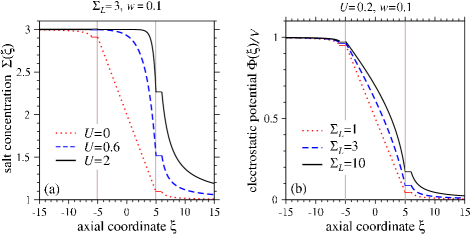
Figure 2: Salt concentration and electrostatic potential across an unimpeded pore of aspect ratio $w=a/d=0.1$. (a) The salt density $\Sigma(\xi)$ as a function of the axial coordinate for various EOF velocities $U$ and salt ratio $\Sigma_{L}=3$. (b) The normalized potential $\Phi(\xi)/V$ for various salt ratios $\Sigma_{L}$.

The spatially varying total salt concentration results in a spatially varying conductivity. Fig. 2(b) shows the resulting electrostatic potential along the axial coordinate $\xi$. For vanishing salt gradient $\Sigma_{L}=1$, Eq. 19 shows the potential decays as $1/r$ in the analyte reservoir, consistent with our assumption of a hemispherical EOF profile far from the pore. In the presence of an imposed salt gradient ($\Sigma_{L}\neq 1$), additional logarithmic terms arise in the reservoir potential $\Phi_{r}(r)$. These results show that although most of the potential drop occurs across the membrane-spanning pore, in the presence of ionic current, the electrostatic potentials in the reservoirs vary slowly with distance from the pore mouths.

For $\Sigma_{L}=1$ and long pores ($w\ll 1$), the potential at the pore mouth in the grounded analyte reservoir $\Phi_{+}\approx wV$ may not be small for sufficiently large applied bias voltage. Furthermore, we will show that the analyte capture rate is sensitive to $\Phi_{+}$ as it depends on the exponent of $\Phi_{+}$. For imposed salt gradients $\Sigma_{L}>1$, the conductivity in the left reservoir is relatively higher and more of the voltage drop occurs across the pore and the analyte (right) reservoir. This further raises the potential $\Phi_{r}(r=1)=\Phi_{+}$ felt by the charged macromolecules at the mouth of the pore in the analyte chamber. Note that the potential $\Phi_{r}(r)$ depends on the gradient of conductivity (arising from the salt concentration gradient), and not on its absolute value. The conductance variation arising from salt concentration gradients provides a simple mechanism by which the potential $\Phi_{r}(r)$ can be increased through the salt ratio $\Sigma_{L}$, enhancing in the capture rate of charged analytes.

III.2 Effect of electroosmotic flows

Now consider how the details of the electroosmotic flow velocity $U$ may affect the electrostatic potential. For an EOF with given magnitude $U$, the potentials $\Phi_{\pm}$ can be calculated from Eqs. 21 and 22. However, recall that the EOF velocity is driven by the potential difference applied across the pore EOF ; therefore, $U$ must be self-consistently solved by finding the root to

$$U=\Gamma(U,\Sigma_{L})(\Phi_{+}[U,\Sigma_{L}]-\Phi_{-}[U,\Sigma_{L}]),$$ (25)

where we have explicitly denoted the dependence of $\Phi_{\pm}$ on $U$ and $\Sigma_{L}$. The prefactor $\Gamma(U,\Sigma_{L})$ measures the effective electroosmotic permeability, which is inversely proportional to the pore length and fluid viscosity, and proportional to the “$\zeta$-potential” EOF . Within the linearized Debye-Hückel theory for electrolytes, this local $\zeta$-potential is proportional to the pore surface charge times the local screening length $\kappa^{-1}(x)$. In our problem where the ionic strength is varying in the axial direction along the pore, the $\zeta-$potential is also varying along the pore. Although a nonuniform surface potential, along with the constraint of fluid incompressibility, can give rise to nonuniform flow within the pore, it has been shown that the net fluid flow across a pore can be found by averaging the $\zeta$-potential (or screening length) across the pore IEEE ; IDOL ; KENNY :

$$\begin{array}[]{rl}\Gamma(U,\Sigma_{L})&\displaystyle\equiv\left({\sigma k_{B}T\over\eta de}\right){1\over d}\int_{-d/2}^{d/2}{\mbox{d}x\over\kappa(x)}\\[13.0pt] &\displaystyle\equiv\Gamma_{R}\,w\int_{-1/(2w)}^{1/(2w)}{\mbox{d}x\over\sqrt{\Sigma_{p}(x)}},\end{array}$$ (26)

where

$$\Gamma_{R}\equiv\left({\sigma\over eac_{R}}\right){w\over\mu\Lambda_{R}^{1/2}}$$

is the dimensionless permeability referenced to the salt in the right chamber. For a typical SiN membrane with constant surface charge density $|\sigma|<1$ microcoulomb/cm² SINCHARGE , a 5nm radius, 40nm length pore in water gives $|\Gamma_{R}|<0.2$.

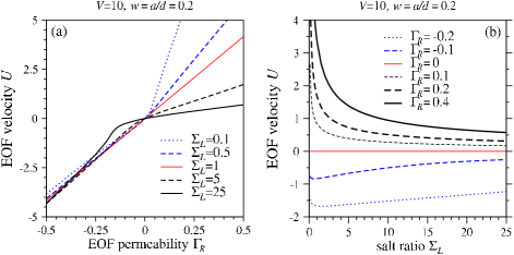
Figure 3: (a) EOF velocity $U$ as a function of effective pore EOF permeability $\Gamma_{R}$. The response deviates from linear for large and small salt ratios. The deviations are most pronounced for $\Gamma_{R}>0$ where EOF is into the right reservoir ($U>0$). (b) EOF velocity as a function of salt ratio for various effective pore surface charge densities. For $\Gamma_{R}>0$, increasing the salt ratio decreases the effective screening length in the pore, reducing the EOF velocity (cf. Eq. 25). When $\Gamma_{R}<0$, the salt in the right reservoir is swept into the left reservoir, keeping the screening length approximately $\kappa^{-1}_{R}$ throughout the pore and very little dependence on $\Sigma_{L}$ arises. In both plots $V=10$ and $w=a/d=0.2$.

Figure 3(a) shows the self-consistent EOF velocity $U$ (obtained by using Eq. 26 and solving Eq. 25) as a function of $\Gamma_{R}$, for various salt ratios $\Sigma_{L}$. For $\Gamma_{R}>0$ and $U>0$, salt is being swept from the left to right reservoirs. When $\Sigma_{L}>1$, the pore feels a higher averaged salt concentration, lowering the $\zeta$-potential, thereby reducing the EOF response to $\Gamma_{R}$. Conversely, when $\Sigma_{L}<1$, a higher $\zeta$-potential and stronger response arises. Fig. 3(b) shows the EOF velocity $U$ as a function of salt ratio $\Sigma_{L}$ for various $\Gamma_{R}$. For $\Sigma_{L}\rightarrow\infty$, $U$ vanishes along with the effective pore $\zeta$-potential.

The pore mouth potential $\Phi_{+}$ felt by the charged analyte is shown in Fig. 4. As a function of pore charge/permeability $\Gamma_{R}$, the potential $\Phi_{+}$ exhibits a maximum(minimum) for $\Sigma_{L}>1(\Sigma_{L}<1)$. This nonmonotonic dependence arises because for $\Sigma_{L}>1$ and small $U\gtrsim 0$, the EOF changes the conductance structure so that $\Phi_{+}$ initially increases. In other words, the largest voltage drop across the analyte (right reservoir) reservoir occurs at small, positive $U$. For larger $U$, high salt is swept well into the right reservoir reducing the effective relative conductivity across the pore. Most of the voltage drop then occurs in regions away from the pore well in the right reservoir, diminishing $\Phi_{+}$ to the value $wV/(2+2w)$ expected in the uniform salt ($\Sigma_{L}=1$) limit. For $\Sigma_{L}<1$, more voltage drop occurs across the left reservoir, reducing $\Phi_{+}$ below $wV/(2+2w)$.

Figure 4: (a). The electrostatic potential in the right reservoir (normalized by the applied potential $V$), as a function of salt asymmetry $\Sigma_{L}$ for various pore EOF permeabilities $\Gamma_{R}$. Here the pore aspect ratio was set to $w=a/d=0.2$. (b) The magnitude of the potential near the mouth pore as a function of EOF permeability $\Gamma_{R}$ for various salt ratios.

Fig. 4(b) shows that as the pore potential $\Phi_{+}$ increases with the salt ratio $\Sigma_{L}$. This is consistent with the observed increase in analyte capture rate with increasing salt in the analyte-free chamber. Also consistent with Fig. 4(a) is the slight increase, then decrease in $\Phi_{+}$ as $\Gamma_{R}$ is increased

III.3 Charged analyte distribution

We now model how both the approximate EOF velocity $\hat{r}U/(2r^{2})$ and the electrostatic potentials (Eqs. 17, 19, and 18) affect the capture of charged analytes to the nanopore as functions of parameters such as the applied salt ratio $\Sigma_{L}$, applied voltage bias $V$, and and pore surface charge/permeability $\Gamma_{R}$. When a charged analyte molecule of size of order $a$ enters the hemispherical cap, it blocks the pore and prevents ion transport. Such a nonspecifically adsorbed particle can spontaneously desorb from the mouth of the pore with rate $k_{\rm off}$. Alternatively, as in the case of DNA, it may translocate through the pore to the opposite, receiving reservoir. Although translocation of a polymer involves many stochastic degrees of freedom, we will lump the process into a single, effective rate $k_{\rm t}$, such that $k_{\rm t}^{-1}$ represents the typical time for the macromolecule to fully tunnel across the pore, allowing ionic current to flow again.

If the hemispherical cap can accommodate at most one blocking macromolecule, its mean field, steady-state occupation $0\leq\theta\leq 1$ is balanced according to:

$$k_{\rm on}\rho(1)(1-\theta)=(k_{\rm off}+k_{\rm t})\theta,$$ (27)

where $\rho(1)\equiv\lim_{r\rightarrow 1^{+}}\rho(r)$ is the analyte concentration just outside the cap region, and $k_{\rm on}$ is its adsorption rate into the hemisphere. To explicitly determine $\theta$ we need to relate the unmeasurable, kinetically-determined $\rho(1)$ with the experimentally imposed macromolecular density $\rho_{\infty}\equiv\rho(r\rightarrow\infty)$. This relationship is obtained by solving the mean field, steady-state convection-diffusion equation for the density in the bulk region:

$$(1-\theta)\nabla\cdot\left[{\bf A}(r)\rho(r)\right]=\nabla^{2}\rho(r),\quad r>1,$$ (28)

where

$${\bf A}(r)=A(r)\hat{r}=\left[{U\over 2Dr^{2}}+q{\partial\Phi_{r}(r)\over\partial r}\right]\hat{r}$$ (29)

is the normalized drift arising from both a hydrodynamic flow and an electrostatic potential induced by electroosmosis and ionic conduction, respectively. The drift induced by the electrostatic potential is proportional to the effective number of electron charges $q$ of the analyte. The factor $(1-\theta)$ reflects our assumption that the EOF flow and ionic current is completely shut off when a macromolecule occupies the cap ($\theta=1$). In writing Eqs. 27 and 28, we have implicitly assumed that the time $\tau_{\rm eff}$ required to form the effective potential $U/(2Dr)+q\partial_{r}\Phi_{r}(r)$ is much less than the typical times associated with dissociation, association, or translocation: $\tau_{\rm eff}\ll k_{\rm off}^{-1},k_{\rm on}^{-1},k_{\rm t}^{-1}$. For relevant parameters, $\tau_{\rm eff}\sim a^{2}/(\Lambda_{R}D)\sim 10^{-10}$s. Provided all the rates are slower than the rate of reestablishing the effective potential, we can assume that the field and flow configurations instantaneously follow those corresponding to whether or not the pore is blocked.

The boundary condition associated with Eq. 28 is applied just outside the hemispherical cap ($r=1^{+}$) and is determined by macromolecular flux balance through the interface ADSORPTION1 ; ADSORPTION2

$$\begin{array}[]{l}D\partial_{r}\rho(r)\big{|}_{r=1^{+}}-(1-\theta)\left[{U\over 2}+Dq\nabla\Phi_{+}\right]\rho(1)\\[13.0pt] \>\hskip 76.82234pt=k_{\rm on}\rho(1)(1-\theta)-k_{\rm off}\theta.\end{array}$$ (30)

Upon solving Eq. 28 for $\rho(r)$ and using Eq. 27 for $\rho(1)$, we find

$$\rho(r)=e^{(1-\theta)\int_{1}^{r}A(y)dy}\left[{k_{\rm t}\theta\over D}\int_{1}^{r}y^{-2}e^{-(1-\theta)\int_{1}^{y}A(y^{\prime})dy^{\prime}}dy+{(k_{\rm off}+k_{\rm t})\theta\over k_{\rm on}(1-\theta)}\right].$$ (31)

After setting $r\rightarrow\infty$ in Eq. 31, we relate the mean cap occupation $\theta$ to the bulk analyte density $\rho_{\infty}$ through the physical solution of the integro-transcendental equation

$${k_{\rm t}\theta\over D}I(\theta)+{(k_{\rm off}+k_{\rm t})\theta\over k_{\rm on}(1-\theta)}e^{(1-\theta)(U/(2D)-q\Phi_{+})}=\rho_{\infty},$$ (32)

where

$$I(\theta)\equiv\int_{1}^{\infty}e^{(1-\theta)\left({U\over 2Dr}-q\Phi_{r}(r)\right)}r^{-2}\mbox{d}r.$$ (33)

When $k_{\rm t}=0$, adsorbed macromolecules do not translocate and can only detach back into the right bulk reservoir. In this limit, $I(\theta)$ does not arise in Eq. 32 and $\theta$ depends only on the value $\Phi_{+}$ of electrostatic potential at the pore mouth. Moreover, the dependence on the normalized macromolecule diffusivity arises only in $U/(2D)$, the drift due to EOF at the pore mouth. Although the EOF and ionic conduction in the fluid arises from nonequilibrium processes, the density profile $\rho(r)$ in the $k_{\rm t}=0$ limit is an equilibrium density self-consistently determined by the effective potential $(1-\theta)\left[U/(2Dr)-q\Phi_{r}(r)\right]$. For parameters such that $A(1)\equiv\left[U/(2D)-Q\Phi_{+}\right]\gg\ln(\rho_{\infty}k_{\rm on}/k_{\rm off})$,

$$\theta\sim\left({k_{\rm on}\over k_{\rm off}}\right)\rho_{\infty}e^{-U/(2D)+q\Phi_{+}}\ll 1.$$ (34)

This form corresponds to an equilibrium “adsorption isotherm” on the single site and depends only on the value of the potential energy at that site.

Conversely, in the limit of high translocation rates such that $k_{\rm t}k_{\rm on}/D\gg k_{\rm off}$ and $\left[U/(2D)-q\Phi_{+}\right]\gg\ln(\rho_{\infty}k_{\rm on}/k_{\rm t})$, the first iteration about $\theta=0$ to Eq. 32 yields

$$\theta\sim{(k_{\rm on}/k_{\rm t})D\rho_{\infty}e^{-U/(2D)+q\Phi_{+}}\over k_{\rm on}I(0)e^{-U/(2D)+q\Phi_{+}}+D}.$$ (35)

Here, the surface density $\rho(1)\sim k_{\rm t}\theta/k_{\rm on}$ resembles that of an adsorbing sphere with an attachment rate $k_{\rm on}$, but modified by the $O(1)$ term $I(0)e^{-U/(2D)+q\Phi_{+}}$ resulting from stochastically switching of the effective drift.

Although the full solution for the pore occupation must be solved numerically, we see that $\theta$ is exponentially sensitive to both the magnitude of the EOF velocity $U$ and the electrostatic potential at the cap $\Phi_{+}$ through an effective drift defined by the combination $U/(2D)-q\Phi_{+}$. Note that both $U$ and $\Phi_{+}$ depend linearly on the bias voltage $V$, but nonlinearly on the salt ratio $\Sigma_{L}$. The EOF velocity $U$ is a function of $\Gamma_{R}$ through the solution Eq. 25, while $\Phi_{+}$ depends indirectly on $\Gamma_{R}$ through the resulting flow velocity $U$ that changes the local conductivity when $\Sigma_{L}\neq 1$. However, only the electrostatic drift $q\Phi_{+}$ depends on the effective analyte charge $q$.

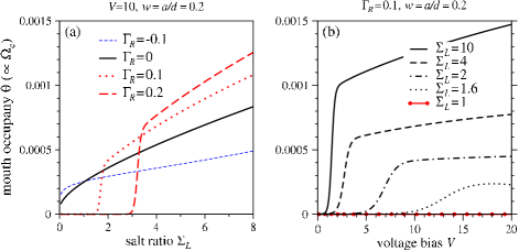
Figure 5: (a) Pore mouth occupation fraction $\theta$ as a function of salt ratio $\Sigma_{L}$ for various EOF permeability $\Gamma_{R}$ and $V=10$. Note the sharp increase in $\theta$ as a function of $\Sigma_{L}$ for positive surface charges. Parameters used were $\rho_{\infty}=10^{-7}$, $V=10$, $w=0.2$, $k_{\rm on}/k_{\rm off}=1000$, and $k_{\rm on}/k_{\rm t}=10^{4}$. For small $\Sigma_{L}$, larger $\Gamma_{R}>0$ induces larger $U>0$, pushing the analyte away. At higher salt $\Sigma_{L}$, the EOF is mitigated due to the reduction in $\zeta$-potential (or effective surface charge) indicated by Eq. 26. The reduction of EOF to modest values allows the attraction from the term $q\Phi_{+}$ to overcome the repulsive effect of the EOF (cf. Fig. 4(a)), increasing $\theta$. (b) Occupation fraction $\theta$ as a function of bias voltage $V$ at different salt ratios and $\Gamma_{R}=0.1$.

Since many analyte capture experiments exhibit infrequent pore blocking, even with bias voltages as high as +250mV ($V\approx+10$), we use parameters that yield small numerical values of $\theta$. Henceforth, we set the relative analyte/ion diffusivity $D=0.01$, $\rho_{\infty}=10^{-7}$ (corresponding to an analyte concentration of $\sim 1$nM for $a\sim 5$nm), and the effective analyte charge $q=30$ (corresponding to that of an approximately 500bp strand of dsDNA DNAQ ). Figure 5 shows representative numerical solutions of Eq. 32 as a function of (a) salt ratio $\Sigma_{L}$, and (b) bias voltage $V$. Fig. 5(a) shows that for larger $\Gamma_{R}$ (larger $U$), the repulsive $U/(2D)$ term dominates in keeping $\theta$ small. However, upon increasing $\Sigma_{L}$, attraction arising from an increasing $q\Phi_{+}$ term eventually increases $\theta$. Larger values of $\Sigma_{L}$ also attenuate the pore-averaged $\zeta$-potential, reducing the repulsive EOF, further increasing $\theta$. For fixed $V$, we will show that the analyte capture rate is proportional to $\theta$; therefore, Fig. 5(a) predicts the capture rate as a function of salt ratio.

To determine how $\theta$ depends on the applied voltage, we use simple assumptions to approximate how the kinetic rates depend on $V$,

$$k_{\rm off}=\omega_{\rm off}e^{-fqV},\,k_{\rm on}=\omega_{\rm on},\,k_{\rm t}=\omega_{\rm t}V,$$

where $\omega_{\rm off},\omega_{\rm on}$ are intrinsic detachment and attachment rates, and $1/\omega_{\rm t}$ is the typical conditional mean time for analyte translocation across the nanopore under a $v\approx k_{B}T$ voltage bias (translocation is assumed negligible when $V=0$ BAYLEY2008 but can be approximated for polymer translocation PORET2 ; PORET3 ). When the macromolecular analyte blocks the pore and $\theta=1$, a fraction $f$ of the $q$ charges may be exposed to the potential in the pore. When the pore is completely blocked, this potential is approximately $V$ since there is no voltage drop across the left reservoir and the pore. For detachment to occur, an energy barrier $fqV$ must be overcome, resulting in $k_{\rm off}\approx\omega_{\rm off}e^{-fqV}$SCHULTENF . In Fig. 5(b), $\theta$ is plotted as a function of voltage $V$ for various fixed salt ratios $\Sigma_{L}$. The kinetic parameters chosen were $f=0.02$, $\omega_{\rm off}=\omega_{\rm on}$, and $\omega_{\rm off}/\omega_{\rm t}=10^{5}$. This choice of intrinsic rates corresponds to approximately 4% of captured analyte being translocated at $V=10$, and 96% detaching back into the bulk analyte reservoir. For the chosen parameters, increasing a small voltage $V$ raises $\theta$ exponentially if there is an appreciable ratio $\Sigma_{L}$ that enhances the positive EOF velocity $U$ to increase $\Phi_{+}$ beyond the repulsion caused by the positive flow $U$. At larger $V$, the larger EOF velocity not only pushes the analyte faster from the pore, but also contributes to reduction in the potential $\Phi_{+}$, resulting in a slower increase in occupation.

III.4 Analyte capture rates

We now define the mean analyte capture rates measured in experiments. The average times that a pore stays open and blocked are

$$T_{\rm o}\approx{1\over k_{\rm on}\rho(1)}={1-\theta\over(k_{\rm off}+k_{\rm t})\theta}\quad\mbox{and}\quad T_{\rm b}\approx{1\over k_{\rm off}+k_{\rm t}},$$ (36)

respectively. The inverse of the mean time between successive capture events defines the capture rate $\omega_{\rm c}$:

$$\omega_{\rm c}\approx{1\over T_{\rm b}+T_{\rm o}}=(k_{\rm off}+k_{\rm t})\theta.$$ (37)

Upon defining the normalized capture rate $\Omega_{\rm c}\equiv\omega_{\rm c}/\omega_{\rm off}$, we formally express

$$\Omega_{\rm c}\equiv\left({\omega_{\rm c}\over\omega_{\rm off}}\right)\approx\left(e^{-fqV}+{\omega_{\rm t}\over\omega_{\rm off}}V\right)\theta,$$ (38)

where the voltage-dependent expressions for $k_{\rm off}$ and $k_{\rm t}$ have been used and the occupation $\theta$ is determined as a function of all physical parameters ($\Gamma_{R},f,q,V,w,\Sigma_{L},\rho_{\infty},\omega_{\rm off},\omega_{\rm on}$, and $\omega_{\rm t}$) by solving Eq. 32, or using Eqs. 34 or 35. Thus, for fixed applied voltage $V$, the capture rate as a function of salt ratio $\Sigma_{L}$ is proportional to $\theta$, and is plotted in Fig. 5(a).

Figure 6(a) shows the normalized capture rate $\Omega_{\rm c}$ as a function of voltage $V$ for different salt ratios $\Sigma_{L}$.

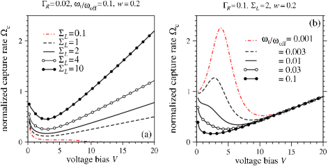
Figure 6: (a) Normalized capture rate $\Omega_{\rm c}$ as a function of bias voltage. (a) The effect of varying salt ratio $\Sigma_{L}$. (b) The effect of varying $k_{\rm on}/k_{\rm t}=\omega_{\rm on}/\omega_{\rm t}$ with fixed $\Sigma_{L}=2$.

For fixed $\Sigma_{L}>1$, increasing $V$ initially decreases $\Omega_{\rm c}$ by virtue of the prefactor $\omega_{\rm off}e^{-fqV}$. Only at larger $V$ does the term $\omega_{\rm t}V/\omega_{\rm off}$ increase the overall capture rate. For small $\Sigma_{L}$, not only is $\Phi_{+}$ slightly decreased, the $\zeta$-potential and EOF are increased, repelling the analyte away from the pore, particularly at high voltages.

Fig. 6(b) plots the capture rate as a function of voltage at various relative translocation rates. For modest $\Gamma_{R}$ and $\Sigma_{L}$, and relatively small translocation rates $\omega_{\rm t}/\omega_{\rm off}$, the initial increase in $\Omega_{\rm c}$ with $V$ arises predominantly from an increase in small $\theta$ (Fig. 5) which decreases $T_{\rm o}$ (Eq. 36) despite the decrease in $k_{\rm off}$. However, for larger $V$, the decrease in $k_{\rm off}$ is not compensated by the slower increase in $\theta$ (Fig. 5). Only at large voltages does the $k_{\rm t}=\omega_{\rm t}V$ term come into play to increase $\Omega_{\rm c}$ linearly. For larger translocation rates $\omega_{\rm t}$, the pore is cleared faster by annihilation of the analyte into the opposing reservoir, preventing the initial increase in $\theta$ with $V$, as well as the initial decrease in $T_{\rm o}$ that would increase the overall capture rate.

IV Summary and Conclusions

We have modeled the underlying electrokinetics to quantitatively describe capture of charged analytes by nanopores in the presence of salt gradients. Our analytic analysis shows that the electrostatic potential near the pore mouth, often neglected, can be sufficient to be an important determinant in the capture of charged particles. We also showed that imposed salt gradients locally change solution conductivity locally, altering the potential distributions. In particular, higher salt (higher conductivity) in the non-analyte chamber decreases the voltage drop in that reservoir and across the nanopore, increasing the analyte blocking probability. As a function of salt ratio, our analysis at small analyte concentrations predicts that both the blocking probability $\theta$ and the capture rate $\Omega_{\rm c}$ always increases as $\Sigma_{L}$ increases. The basic mechanism provides a physically consistent and testable explanation for recently observed increases in capture rate with salt ratio $\Sigma_{L}>1$ MELLERABS .

Electroosmotic flow also affects analyte capture. By itself, hydrodynamic flow (e.g., from electroosmosis) into the analyte reservoir sweeps particles away from the pore, dramatically lowering the blocking probability. However, when the non-analyte chamber contains a higher salt concentration such that $\Sigma_{L}>1$, the same repelling fluid flow can also change the local conductivity structure such that the potential $\Phi_{+}$ felt by the charged analyte at the pore mouth initially increases with flow rate. For small pore charge/permeability $\Gamma_{R}$, we find that repelling EOF actually increases the overall attraction of charged analytes, particularly when $\Sigma_{L}$ and the effective analyte charge $q$ are large. Finally, our analysis shows that the capture rate is sensitive to the translocation rate $\omega_{\rm t}$. When $\omega_{\rm t}\gg\omega_{\rm off}$, and nearly all captured particles are annihilated via translocation into the receiving reservoir, the capture rate increases with bias voltage $V$, except at very low $V$.

We considered only outer solutions, accurate in regions where $Q({\bf r})\approx 0$ outside the charged boundary layer at the solution-membrane interface. However, since we focus on the capture of analyte from the bulk reservoir, the main factor is the voltage drop across the pore with other electrostatic details within the pore relatively unimportant. Although our outer solutions do not hold inside pores with small radii $a<\kappa_{R}^{-1}$, the ionic current flow across such pores still induces a slowly decaying electrostatic potential $\Phi_{r}(r)$ in the bulk analyte chamber, albeit with a small amplitude determined by an effective, small pore aspect ratio $w$. The correspondingly smaller potential $\Phi_{r}(r)$ in the right chamber would give a smaller capture rate at the same analyte density. We expect the analyte capture rate by smaller pores to have the same functional dependences as in our mathematical model, but with a smaller effective $w$. Note that the EOF velocity $U$ is proportional to $w^{2}$ (through $\Gamma(U,\Sigma_{L})$ in Eq. 26), while $\Phi_{+}$ scales as $w$. Therefore, we also expect EOF to become less important than direct electrostatic effects for sufficiently small pores.

In addition to the charge-neutral approximation, our analysis relies on a number of other assumptions, including an effective analyte charge $q$ and pore surface charge $\sigma$ that are independent of the local ionic strength $\Sigma({\bf r})$. Moreover, we have assumed right-cylindrical pores, that the occupation and bulk analyte density can be approximated using a mean field assumption, and that the molecular details of the capture and translocation can be described using simple kinetic rates. Although some of these assumptions can be lifted in more detailed models and numerical analyses (for example, in a model of conical pores CONICAL ), our simple model embodies the essential physics of the problem and we expect our results to be qualitatively predictive.

Acknowledgments This work was supported by the NSF through grant DMS-0349195, and by the NIH through grant K25AI41935.

References

- (1) Maglia G, Restrepo, MR, Mikhailova E, and Bayley H (2008) Enhanced translocation of single DNA molecules through -hemolysin nanopores by manipulation of internal charge. Proc. Natl Acad. Sci. USA 105:19720-19725.
- (2) Gershow M and Golovchenko JA (2007) Recapturing and trapping single molecules with a solid-state nanopore. Nature Nanotechnology 2:775-779.
- (3) Tabard-Cossa V, Trivedi D, Wiggin M, Jetha NN, and Marziali A (2007) Noise analysis and reduction in solid-state nanopores. Nanotechnology 18:1-6.
- (4) Strom AJ et al. (2005) Fast DNA Translocation through a Solid-State Nanopore. Nano Lett. 5:1193-1197.
- (5) Meller A (2008) Sensing biomolecules translocation dynamics with solid state nanopores. PHYS 178, The 236th ACS National Meeting, Philadelphia, PA, August 17-21, 2008
- (6) Wanunu M, Cohen-Karni D, Sutin J and Meller A (2008) Nanopore Analysis of Biopolymers under Physiological Ionic Strengths. Biophys. J. 94:51 (Meeting Abstract)
- (7) Flomenbom O and Klafter J (2003) Single stranded DNA translocation through a nanopore: A master equation approach. Phys. Rev. E 68:041910.
- (8) Aksimentiev A, Heng JB, Timp G, and Schulten K (2004) Microscopic Kinetics of DNA Translocation through Synthetic Nanopores. Biophys. J. 87:2086-2097.
- (9) Park PJ and Sung W (1998) Polymer translocation induced by adsorption J. Chem. Phys. 108:3013-3018.
- (10) Singer A, Gillespie D, Norbury J, and Eisenberg RS (2008) Singular perturbation analysis of the steady state Poisson-Nernst-Planck system: applications to ion channels. Eur. J. Appl. Math. 9:541-560.
- (11) Chen, D, Lear J, and Eisenberg RS (1997) Permeation through an Open channel. Poisson-Nernst-Planck Theory of a Synthetic Ionic Channel. Biophys. J. 72:97-116.
- (12) Wong CTA and Muthukumar M (2007) Polymer capture by electro-osmotic flow of oppositely charged nanopores. J. Chem. Phys. 126:164903.
- (13) Chen DP, Barcilon V, and Eisenberg RS (1992) Constant fields and constant gradients in open ionic channels. Biophys. J. 61:1372-1393.
- (14) Dagan Z, Weinbaum S, and Pfeffer R (1982) An infinite-series solution for the creeping motion through an orifice of finite length. J. Fluid Mech. 115:505-523.
- (15) Parmet IL and Saibel E (1965) Axisymmetric creeping flow from an orifice in a plane wall. Comm. Pure & Appl. Math. XVIII:17-23.
- (16) Kelman RB (1965) Steady-state diffusion through a finite pore into an infinite reservoir: An exact solution. Bull. Mathematical Biophys. 27:57-65.
- (17) Rice CL and Whitehead R (1965) Electrokinetic Flow in a Narrow Cylindrical Capillary. J. Phys. Chem. 69:4017-4024.
- (18) Ji F, Zuo C, Zhang P, Zhou D (2005) Analysis of Electroosmotic Flow with Linear Variable Zeta Potential Proc. 2005 Int. Conf. on MEMS,NANO, and Smart Systems (ICMENS’05).
- (19) Anderson JL, Idol WK (1985) Electroosmosis through pores with nonuniformly charged walls Chem. Eng. Commun. 38:93-106.
- (20) Herr AE, Molho JI, Santiago JG, Mungal MG, Kenny TW, Garguilo MG (2000) Electroosmotic Capillary Flow with Nonuniform Zeta Potential Anal. Chem. 72:1053-1057.
- (21) Whitman PK and Feke DL (1988) Comparison of the Surface Charge Behavior of Commercial Silicon Nitride and Silicon Carbide Powders. J. Am. Ceram. Soc. 71:1086-1093.
- (22) Chou T and D’Orsogna MR (2007) Multistage adsorption of diffusing macromolecules and viruses. J. Chem. Phys. 127:105101
- (23) Diamant H, Ariel G, and Andelman D (2001) Kinetics of surfactant adsorption: the free energy approach. Colloids Surf. A 183-185:259
- (24) Smith SB and Bendich AJ (1990) Electrophoretic charge density and persistence length of DNA as measured by fluorescence microscopy. Biopolymers 29:1167-1173.
- (25) Lakatos G, Chou T, Bergersen B, and Patey GN (2005) First passage times of driven DNA hairpin unzipping. Physical Biology 2:166-174.
- (26) Grosberg AY, Nechaev S, Tamm M, and Vasilyev O (2006) How Long Does It Take to Pull an Ideal Polymer into a Small Hole? Phys. Rev. Lett. 96:228105
- (27) Heng JB, et al. (2005) Beyond the Gene Chip Bell labs Technical Journal 10:5-22.
- (28) Cervera J, Schiedt B, and Ramirez P (2005) A poisson/Nernst-Planck model for ionic transport through synthetic conical nanopores. Europhys. Lett. 71:35-41.