Macroscopic Quantum Tunneling Effect of $Z_{2}$ Topological Order

Abstract

In this paper, macroscopic quantum tunneling (MQT) effect of $Z_{2}$ topological order in the Wen-Plaquette model is studied. This kind of MQT is characterized by quantum tunneling processes of different virtual quasi-particles moving around a torus. By a high-order degenerate perturbation approach, the effective pseudo-spin models of the degenerate ground states are obtained. From these models, we get the energy splitting of the ground states, of which the results are consistent with those from exact diagonalization method.

I Introduction

In quantum mechanics, quantum tunneling effect is a process by which quantum particles penetrate barriers, which are forbidden in classical processes Razag . It is Gamov who pointed out that a single $\alpha$ particle can tunnel through a barrier which introduced ”macroscopic quantum tunneling” (MQT) into physics firstly. Macroscopic quantum tunneling effects have been widely applied to different research fields, such as quantum oscillations between two degenerate wells of NH₃, quantum coherence in one dimension charge density waves, macroscopic quantum tunneling effect in ferromagnetic single domain magnets and quantum tunneling phenomena in biased Josephson junctions. In general, to find MQT in a system, there must exist two or more separated ”classical” states with macroscopically distinct. As shown in Fig.1, a quantum particle may take a short cut from one well to the other without climbing the barrier.

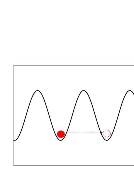
Figure 1: The scheme of a typical macroscopic quantum tunneling process.

In this paper we will study a new class of MQT - the MQT in $Z_{2}$ topological order. At the beginning we give a brief introduction to $Z_{2}$ topological order. Topological order is a new type of quantum orders beyond Landau’s symmetry breaking paradigmwen ; wen1 ; wen3 ; wen4 ; wen5 , of which there are four universal properties : 1) All excitations have mass gap; 2) The quantum degeneracy of the ground states depends on the genius of the manifold of the background; 3) There are (closed) string net condensations; 4) Quasi-particles have exotic statistics. All these properties are robust against perturbations. $Z_{2}$ topological order is the simplest topological ordered state with three types of quasiparticles: $Z_{2}$ charge, $Z_{2}$ vortex, and fermionswen4 . $Z_{2}$ charge and $Z_{2}$ vortex are all bosons with mutual $\pi$ statistics between them. The fermions can be regarded as bound states of a $Z_{2}$ charge and a $Z_{2}$ vortex. In last ten years, several exactly solvable spin models with $Z_{2}$ topological orders were found, such as the Kitaev toric-code model k1 , the Wen-plaquette modelwen4 ; wen5 and the Kitaev model on honeycomb latticek2 .

A decade ago, Kitaev pointed out that the degenerate ground states of a $Z_{2}$ topological order make up a protected code subspace (the so-called toric-code) free from errork1 ; k2 . In Ref.ioffe , topological qubit based on the degenerate ground states of a $Z_{2}$ topological order has been designed. Then one can manipulate the degenerate ground states by braiding anyons, which has becomes a hot issue recently pa ; sarma ; du1 ; zoller ; vid ; vids ; zhang ; zhang1 ; gao ; kou1 ; kou1' ; vid1 ; vid2 . Recently, an alternative approach to design TQC is proposed by manipulating the protected code subspacekou1 ; kou1' . The key point to manipulate the degenerate ground states is to tune their MQT effect. Thus it becomes an interesting issue to study the MQT in $Z_{2}$ topological order.

In this paper, by using a high-order degenerate perturbative approach, we study the MQT of the degenerate ground states of $Z_{2}$ topological order, taking the Wen-plaquette Model as an example. The remainder of the paper is organized as follows. In Sec. II, the degenerate ground states of the Wen-plaquette model is classified by the topological closed string operators. In Sec.III, the dynamics of quasi-particles are studied. In Sec. IV, the MQT of the degenerate ground states of the $Z_{2}$ topological order are formalized on a torus of different lattices. The numerical results are given to compare with the theoretical results. Finally, the conclusions are given in Sec. V.

II The degenerate ground states and its representation of string operators

In this section, we study the degenerate ground states of the Wen-plaquette model. The Hamiltonian of the Wen-plaquette model is given by

$$\hat{H}=-g\sum_{i}\hat{F}_{i},$$ (1)

with

$$\hat{F}_{i}=\sigma_{i}^{x}\sigma_{i+\hat{e}_{x}}^{y}\sigma_{i+\hat{e}_{x}+\hat{e}_{y}}^{x}\sigma_{i+\hat{e}_{y}}^{y}$$ (2)

and $g>0.$ $\sigma_{i}^{x},$ $\sigma_{i}^{y}$ are Pauli matrices on site $i.$ The ground states of the Wen-plaquette model denoted by ${F_{i}\equiv+1}$ at each site are known to be an example of $Z_{2}$ topological state. The ground state energy becomes $E_{0}=-gN$ where $N$ is the total lattice numberwen ; wen4 ; wen5 ; kou2 .

In the topological order of the Wen-plaquette model, there exist three types of open string operators $W_{c}(C)$, $W_{v}(C)$, $W_{f}(C)$ corresponding to three types of quasi-particles: $Z_{2}$ charge, $Z_{2}$ vortex, and fermion, respectivelywen1 . Here $C$ is a (closed or open) loop. To create a $Z_{2}$ vortex (charge) excitation, one may draw a string state that connects nearest neighboring even (odd) plaquettes $W_{v}(C)$ (or $W_{c}(C)$). Such a string state is created by the following string operator $\prod_{C}\sigma_{i}^{a_{i}}$ where the product $\prod_{C}$ is over all the sites on the string along a loop $C$ connecting even-plaquettes (or odd-plaquettes), $a_{i}=y$ if $i$ is even and $a_{i}=x$ if $i$ is odd. For a fermionic excitation, the string operator has a form as $W_{f}(C)=\prod_{n}\sigma_{i_{n}}^{l_{n}}$ with a string $C$ connecting the mid-points of the neighboring links, and $i_{n}$ are sites on the string. $l_{m}=z$ if the string does not turn at site $i_{m}$. $l_{m}=x$ or $y$ if the string makes a turn at site $i_{m}$. $l_{m}=y$ if the turn forms a upper-right or lower-left corner. $l_{m}=x$ if the turn forms a lower-right or upper-left corner. It is obvious that the fermionic string can be regarded as a bound state of strings of the $Z_{2}$ charges and the $Z_{2}$ vortices, that is $W_{f}(C)=W_{c}(C)W_{v}(C)$. If $C$ are closed loops, we get condensed closed-string operators of the ground states $|\Psi_{0}\rangle$ as

$$\langle\Psi_{0}|W_{c}(C)|\Psi_{0}\rangle = 1,\text{ }\langle\Psi_{0}|W_{v}(C)|\Psi_{0}\rangle=1,$$ (3)

$$\langle\Psi_{0}|W_{f}(C)|\Psi_{0}\rangle = 1.$$

One can see the detailed definition of the string operators in Ref.wen1 .

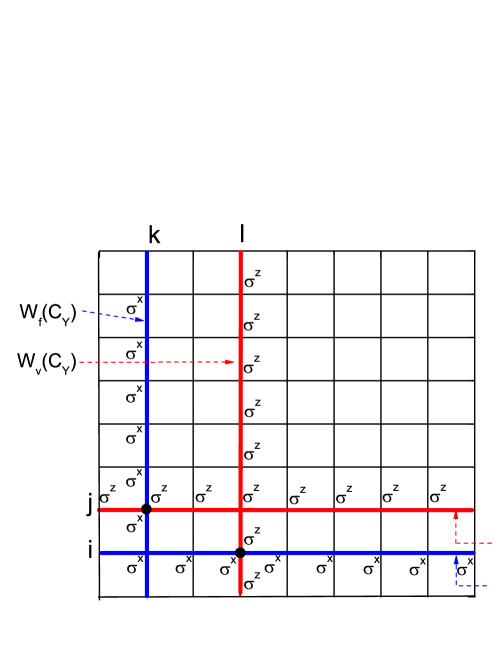
Figure 2: The topological closed string operators on a torus. The dots denote the crosses of different types of strings.

To classify the degeneracy of the ground states, we define three types of topological closed-string operators $W_{c}(\mathcal{C}),$ $W_{v}(\mathcal{C})$ and $W_{f}(\mathcal{C})=W_{c}(\mathcal{C})W_{v}(\mathcal{C})$, with $\mathcal{C}$ denoting topological closed loops. The word ^′topological^′ means that the ^′big^′ loops $\mathcal{C}$ surround the torus globally (See Fig.2). One can easily check the commutation relations between the topological closed string operators and the Hamiltonian

$$\left[H,\text{ }W_{c}(\mathcal{C})\right]=\left[H,\text{ }W_{v}(\mathcal{C})\right]=\left[H,\text{ }W_{f}(\mathcal{C})\right]=0.$$ (4)

For the ground states on a torus of an even-by-even ($e\ast e$) lattice, we can define four types of elementary topological closed string operators, $W_{v}(\mathcal{C}_{X}),$ $W_{v}(\mathcal{C}_{Y}),$ $W_{f}(\mathcal{C}_{X})$ and $W_{f}(\mathcal{C}_{Y}).$ Here $\mathcal{C}_{X}$ denotes a closed-loop around the torus along $e_{x}$-direction and $\mathcal{C}_{Y}$ denotes a closed loop around the torus along $e_{y}$-direction. Due to the commutation (or anti-commutation) relations between them

$$\left[W_{v}(\mathcal{C}_{X}),W_{f}(\mathcal{C}_{X})\right] = 0,\text{ }\left[W_{v}(\mathcal{C}_{Y}),W_{f}(\mathcal{C}_{Y})\right]=0,$$ (5)

$$\left[W_{v}(\mathcal{C}_{X}),W_{v}(\mathcal{C}_{Y})\right] = 0,\text{ }\left[W_{f}(\mathcal{C}_{X}),W_{f}(\mathcal{C}_{Y})\right]=0,$$

$$\left\{W_{v}(\mathcal{C}_{X}),W_{f}(\mathcal{C}_{Y})\right\} = 0,\text{ }\left\{W_{v}(\mathcal{C}_{Y}),W_{f}(\mathcal{C}_{X})\right\}=0,$$

we may identify $W_{v}(\mathcal{C}_{X}),$ $W_{v}(\mathcal{C}_{Y}),$ $W_{f}(\mathcal{C}_{X})$ and $W_{f}(\mathcal{C}_{Y})$ by pseudo-spin operators $\tau_{1}^{x},$ $\tau_{2}^{x}$ $\tau_{2}^{z},$ and $\tau_{1}^{z}$ as

$$W_{v}(\mathcal{C}_{X}) = \tau_{1}^{x}\otimes\mathbf{1},\text{ }W_{v}(\mathcal{C}_{Y})\rightarrow\mathbf{1}\otimes\tau_{2}^{x},$$ (6)

$$W_{f}(\mathcal{C}_{X}) \rightarrow \mathbf{1}\otimes\tau_{2}^{z},\text{ }W_{f}(\mathcal{C}_{Y})\rightarrow\tau_{1}^{z}\otimes\mathbf{1}.$$

Thus other five topological closed string operators $W_{c}(\mathcal{C}_{X}),$ $W_{c}(\mathcal{C}_{Y}),$ $W_{c}(\mathcal{C}_{XY}),$ $W_{v}(\mathcal{C}_{XY})$ and $W_{f}(\mathcal{C}_{XY})$ are denoted by $\tau_{1}^{x}\otimes\tau_{2}^{z},$ $\tau_{1}^{z}\otimes\tau_{2}^{x},$ $\tau_{1}^{y}\otimes\tau_{2}^{y},$ $\tau_{1}^{x}\otimes\tau_{2}^{x}$ and $\tau_{1}^{z}\otimes\tau_{2}^{z}$, respectively,

$$W_{c}(\mathcal{C}_{X}) \rightarrow \tau_{1}^{x}\otimes\tau_{2}^{z},\text{ }W_{c}(\mathcal{C}_{Y})\rightarrow\tau_{1}^{z}\otimes\tau_{2}^{x},$$ (7)

$$W_{c}(\mathcal{C}_{XY}) \rightarrow \tau_{1}^{y}\otimes\tau_{2}^{y},\text{ }W_{v}(\mathcal{C}_{XY})\rightarrow\tau_{1}^{x}\otimes\tau_{2}^{x},$$

$$W_{f}(\mathcal{C}_{XY}) \rightarrow \tau_{1}^{z}\otimes\tau_{2}^{z}.$$

Here $\mathcal{C}_{XY}$ is a closed loop around the torus along diagonal directions. In the table.(I), the pseudo-spin representation of the topological closed string operators are illustrated.

Pesudo-spin operators	$\mathcal{C}_{X}$	$\mathcal{C}_{Y}$	$\mathcal{C}_{XY}$
$Z_{2}$-vortex	$\tau_{1}^{x}\otimes\mathbf{1}$	$\mathbf{1}\otimes\tau_{2}^{x}$	$\tau_{1}^{x}\otimes\tau_{2}^{x}$
$Z_{2}$-charge	$\tau_{1}^{x}\otimes\tau_{2}^{z}$	$\tau_{1}^{z}\otimes\tau_{2}^{x}$	$\tau_{1}^{y}\otimes\tau_{2}^{y}$
$Fermion$	$\mathbf{1}\otimes\tau_{2}^{z}$	$\tau_{1}^{z}\otimes\mathbf{1}$	$\tau_{1}^{z}\otimes\tau_{2}^{z}$

Table 1: Pseudo-spin representation of the topological closed string operators on an even-by-even lattice.

Then as the eigenstates of $\tau_{l}^{z}$ ($l=1,2$), the four degenerate ground states are denoted by $\mid m_{1},m_{2}\rangle=\mid m_{1}\rangle\otimes\mid m_{2}\rangle$. For $m_{l}=0,$ we have

$$\tau_{l}^{z}\mid m_{l}\rangle=\mid m_{l}\rangle,$$ (8)

and for $m_{l}=1$ we have

$$\tau_{l}^{z}\mid m_{l}\rangle=-\mid m_{l}\rangle.$$ (9)

Physically, the topological degeneracy arises from presence or the absence of $\pi$ flux of fermion through the hole. The values of $m_{l}$ reflect the presence ($m_{l}=1$) or the absence ($m_{l}=0$) of the $\pi$ flux in the hole.

For the degenerate ground states on an even-by-odd ($e\ast o$) lattice, the situation changes. Because a $Z_{2}$ vortex or $Z_{2}$ charge has to move even steps to go back to the same plaquette around a torus, we cannot well define a topological closed string operator of $Z_{2}$ vortex or $Z_{2}$ charge along $e_{y}$-direction, of which the loop consists of odd number plaquettes. So we can only define topological closed string operator of $Z_{2}$ vortex and $Z_{2}$ charge along $e_{x}$-direction $W(\mathcal{C}_{X})$ ($W(\mathcal{C}_{X})=W_{v}(\mathcal{C}_{X})=W_{c}(\mathcal{C}_{X})$) and the corresponding fermionic string operator along $e_{y}$-direction $W_{f}(\mathcal{C}_{Y}).$ Due to the anti-commutation relations between $W(\mathcal{C}_{X})$ and $W_{f}(\mathcal{C}_{Y})$,

$$\left\{W(\mathcal{C}_{X}),\text{ }W_{f}(\mathcal{C}_{Y})\right\}=0,$$ (10)

we may represent $W(\mathcal{C}_{X})$ and $W_{f}(\mathcal{C}_{Y})$ by pseudo-spin operators $\tau_{1}^{x}$ and $\tau_{1}^{z}$, respectively

$$W(\mathcal{C}_{X})\rightarrow\tau_{1}^{x},\text{ }W_{f}(\mathcal{C}_{Y})\rightarrow\tau_{1}^{z}.$$ (11)

Therefore there are two degenerate ground states $\mid m_{1}\rangle$ that are the eigenstates of $\tau_{1}^{z}$. In the table.(II), the pseudo-spin representation of the topological closed string operators on $e\ast o$ lattice are shown.

Pesudo-spin operators	$\mathcal{C}_{X}$	$\mathcal{C}_{Y}$	$\mathcal{C}_{XY}$
$Z_{2}$-vortex	$\tau_{1}^{x}$	$-$	$\tau_{1}^{x}$
$Z_{2}$-charge	$\tau_{1}^{x}$	$-$	$\tau_{1}^{x}$
$Fermion$	$1$	$\tau_{1}^{z}$	$\tau_{1}^{z}$

Table 2: Pseudo-spin representation of the topological closed string operators on an even-by-odd lattice.

Similarly, for the degenerate ground states on an odd-by-even ($o\ast e$) lattice there are also two types of closed string operators, $W(\mathcal{C}_{Y})$ ($W(\mathcal{C}_{Y})=W_{v}(\mathcal{C}_{Y})=W_{c}(\mathcal{C}_{Y})$) and $W_{f}(\mathcal{C}_{X})$, which can be described by pseudo-spin operators $\tau_{2}^{x}$ and $\tau_{2}^{z}.$ Therefore, the two degenerate ground states on an $o\ast e$ lattice are denoted by $\mid m_{2}\rangle$ which are the eigenstates of $\tau_{2}^{z}.$

For the degenerate ground states on an odd-by-odd ($o\ast o$) lattice, since the total lattice number is odd, we cannot well define $Z_{2}$ vortex or $Z_{2}$ charge globally any more. Instead, we can only define a mixed topological closed-string operator, $W(\mathcal{C}_{XY})=\prod_{\mathcal{C}}\sigma_{i}^{a_{i}}$ where the product $\prod_{\mathcal{C}}$ is over all the sites on the string along a diagonal loop $\mathcal{C}$ connecting plaquettes. The index $a_{i}=x$ or $y$ is determined by the position of the plaquettes. Because $W(\mathcal{C}_{XY})$ anti-commutes with $W_{f}(\mathcal{C}_{X})$ and $W_{f}(\mathcal{C}_{Y})$,

$$\left\{W(\mathcal{C}_{XY}),\text{ }W_{f}(\mathcal{C}_{X})\right\}=0,\text{ }\left\{W(\mathcal{C}_{XY}),\text{ }W_{f}(\mathcal{C}_{Y})\right\}=0,$$ (12)

we may represent $W(\mathcal{C}_{XY})$ and $W_{f}(\mathcal{C}_{X})$ (or $W_{f}(\mathcal{C}_{Y})$) by pseudo-spin operators $\tau^{x}$ and $\tau^{z}$, respectively

$$W(\mathcal{C}_{XY}) \rightarrow \tau^{x},$$

$$W_{f}(\mathcal{C}_{X}) = W_{f}(\mathcal{C}_{Y})\rightarrow\tau^{z}.$$

It is noted that

$$W_{f}(\mathcal{C}_{XY})=W_{f}(\mathcal{C}_{X})W_{f}(\mathcal{C}_{Y})=1.$$ (13)

Thus the two degenerate ground states on an $o\ast o$ lattice $\mid m\rangle$ are the eigenstates of $\tau^{z}$. In the table.(III), the pseudo-spin representation of the topological closed string operators on $o\ast o$ lattice are shown.

Pesudo-spin operators	$\mathcal{C}_{X}$	$\mathcal{C}_{Y}$	$\mathcal{C}_{XY}$
$Z_{2}$-vortex ($Z_{2}$-charge)	$-$	$-$	$\tau^{x}$
$Fermion$	$\tau^{z}$	$\tau^{z}$	$1$

Table 3: Pseudo-spin representation of the topological closed string operators on an odd-by-odd lattice.

As a result, the degeneracy $\mathcal{Q}$ of the ground states of the Wen-plaquette model on lattices with periodic boundary condition (on a torus) is dependent on the lattice numbers : $\mathcal{Q}=4$ on $e\ast e$ lattice, $\mathcal{Q}=2$ on other cases ($e\ast o$, $o\ast e$ and $o\ast o$ lattices)wen ; wen4 ; wen5 ; kou1 ; kou1' ; kou2 .

III Properties of quasi-particles of the Wen-plaquette model

In this section we study the properties of the quasi-particles of the Wen-plaquette model. In this model, $Z_{2}$ vortex is defined as ${F_{i}=-1}$ at even sub-plaquette and $Z_{2}$ charge is ${F_{i}=-1}$ at odd sub-plaquette. The energy gap of $Z_{2}$ charge and $Z_{2}$ vortex is $2g$. The fermions that are the bound states of a $Z_{2}$ charge and a $Z_{2}$ vortex on two neighbor plaquettes have an energy gap of $4g$. All quasi-particles in such an exactly solvable model have flat bands. The energy spectrums are $E_{v}=E_{c}=2g$ for $Z_{2}$ vortex and $Z_{2}$ charge, $E_{f}=4g$ for fermions, respectively. In other words, the quasi-particles cannot move at all. In particular, there exist two types of fermions : the fermions on the vertical links and the fermions on the parallel links.

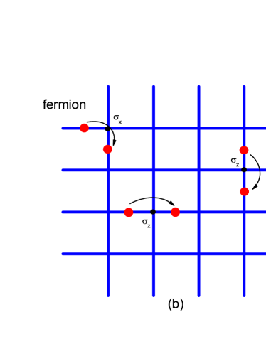
Figure 3: The hoppings of $Z_{2}$ vortex, $Z2$ charge and fermions. The shadow plaquettes, the striped plaquettes and the dots on the links represent $Z_{2}$ vortices, $Z_{2}$ charges and fermions, respectively.

Under the perturbation

$$H_{I}=h^{x}\sum\limits_{i}\sigma_{i}^{x}+h^{z}\sum\limits_{i}\sigma_{i}^{z},$$ (14)

the quasi-particles ($Z_{2}$ vortex, $Z_{2}$ charge and fermion) begin to hopzoller ; vid ; vids ; vid1 ; vid2 ; kou1 ; kou1' ; kou0 . The term $h^{x}\sum\limits_{i}\sigma_{i}^{x}$ drives the $Z_{2}$ vortex, $Z_{2}$ charge and fermion hopping along diagonal direction $\hat{e}_{x}-\hat{e}_{y}$ (See Fig.3(a)). For example, for a $Z_{2}$ vortex living at $i$ plaquette ${F_{i}=-1,}$ when $\sigma_{i}^{x}$ acts on $i+\hat{e}_{x}$ site, it hops to $i+\hat{e}_{x}-\hat{e}_{y}$ plaquette denoted by ${F_{i+\hat{e}_{x}-\hat{e}_{y}}=-1,}$

$${F_{i}}{=-1\rightarrow F_{i}=+1,}\text{ }{F_{i+\hat{e}_{x}-\hat{e}_{y}}}{=+1\rightarrow F_{i+\hat{e}_{x}-\hat{e}_{y}}=-1}\text{.}$$ (15)

A pair of $Z_{2}$ vortices at $i$ and $i+\hat{e}_{x}-\hat{e}_{y}$ plaquettes can be created or annihilated by the operation of $\sigma_{i}^{x}$,

$${F_{i}}{=+1\rightarrow F_{i}=-1,}\text{ }F{{}_{i+\hat{e}_{x}-\hat{e}_{y}}}{=+1\rightarrow F_{i+\hat{e}_{x}-\hat{e}_{y}}=-1.}$$ (16)

The term $h^{z}\sum\limits_{i}\sigma_{i}^{z}$ drive fermion hopping along $\hat{e}_{x}$ and $\hat{e}_{y}$ directions without affecting $Z_{2}$ vortex and $Z_{2}$ charge : the fermions on the vertical links move along vertical directions and the fermions on the parallel links move along parallel directions. With the help of the term $h^{x}\sum\limits_{i}\sigma_{i}^{x},$ the two types of fermions are mixed and the fermions may turn round from vertical links to parallel links (See Fig.3(b)).

A fact is that the topological closed string operators can be considered as quantum tunneling processes of virtual quasi-particle moving along the same loops. Let us take the quantum tunneling process of $Z_{2}$ vortex as an example : at first a pair of $Z_{2}$ vortices are created. One $Z_{2}$ vortex propagates around the torus driven by operators $\sigma_{i}^{x}$ and annihilates with the other $Z_{2}$ vortex. Then a string of $\sigma_{i}^{x}$ is left on the tunneling path, which is just the topological closed string operator $W_{v}(\mathcal{C})$. Such a process effectively adds a unit of a $\pi$-flux to one hole of the torus and changes $m_{l}$ by $1$.

IV Macroscopic quantum tunneling effects of the degenerate ground states

It is known that the degenerate ground states of $Z_{2}$ topological orders have the same energy in the thermodynamic limit. The different ground states can not mix into each other through any local fluctuations. However, in a finite system,  the degeneracy of the ground states can be (partially) removed due to quantum tunneling processes, of which virtual quasi-particles move around the torusk1 ; wen ; ioffe ; kou1 ; kou1' . In general cases, one will get large energy gaps for all quasi-particles and very tiny energy splitting of the degenerate ground states $\Delta E$. Based on such condition, we may ignore high energy excited states and consider only the degenerate ground states. Thus in the following parts we only focus on the ground states that are a four-level (or two-level) system.

IV.1 The high-order degenerate perturbation theory

To solve quantum tunneling problems, people have developed many approaches including the well known WKB (Wentzel, Kramers and Brillouin) method and the instanton approach lately. However, based on semi-classical approximation both above approaches are not available to the MQT of $Z_{2}$ topological order. Instead, in this part, we develop a high-order degenerate perturbative approach to calculate the MQT.

The Hamiltonian of the Wen-plaquette model under the external field has a form as

$$\hat{H}=\hat{H_{0}}+\hat{H}_{I}$$ (17)

in which $\hat{H_{0}}=-g\sum_{i}\sigma_{i}^{x}\sigma_{i+\hat{e}_{x}}^{y}\sigma_{i+\hat{e}_{x}+\hat{e}_{y}}^{x}\sigma_{i+\hat{e}_{y}}^{y}$ is the unperturbation term, and $\hat{H}_{I}=h^{x}\sum\limits_{i}\sigma_{i}^{x}+h^{z}\sum\limits_{i}\sigma_{i}^{z}$ is the small perturbation one. For simplicity, we consider the quantum tunneling process between two degenerate ground states $\mid m\rangle$ and $\mid n\rangle,$

$$\mid m\rangle\Leftrightarrow\mid n\rangle.$$ (18)

According to the Gell-Mann-Low theory, we define a transformation operator $\hat{U_{I}}(0,-\infty)$ as

$$\hat{U_{I}}(0,-\infty)=\mathrm{T}\exp(-i\int_{-\infty}^{0}\hat{H}_{I}^{\prime}(t^{\prime})dt^{\prime})$$ (19)

where

$$\hat{H}_{I}^{\prime}(t)=e^{i\hat{H_{0}}t}\hat{H}_{I}e^{-i\hat{H_{0}}t}.$$ (20)

Here $\mathrm{T}$ denotes a time order and $\hslash=1$. Then the transformation operator $\hat{U_{I}}(0,-\infty)$ in Eq.(19) can be written as

$$\hat{U_{I}}(0,-\infty)\left|m\right\rangle=\sum\limits_{j=0}^{\infty}\hat{U}_{I}^{(j)}(0,-\infty)\left|m\right\rangle,$$ (21)

where

$$\hat{U}_{I}^{(0)}(0,-\infty)\left|m\right\rangle = \left|m\right\rangle,$$

$$\hat{U}_{I}^{(1)}(0,-\infty)\left|m\right\rangle = -i\int_{-\infty}^{0}\hat{H}_{I}^{\prime}(t)dt\left|m\right\rangle$$

$$= \frac{1}{E_{0}-\hat{H_{0}}}\hat{H}_{I}\left|m\right\rangle,$$

$$\hat{U}_{I}^{(2)}(0,-\infty)\left|m\right\rangle = -i\int_{-\infty}^{0}\hat{H}_{I}^{\prime}(t)\hat{U}_{I}^{(1)}(0,-\infty)dt\left|m\right\rangle$$

$$= \frac{1}{E_{0}-\hat{H_{0}}}\hat{H}_{I}\frac{1}{E_{0}-\hat{H_{0}}}\hat{H}_{I}\left|m\right\rangle,$$

$$\hat{U}_{I}^{(j\neq 0)}(0,-\infty)\left|m\right\rangle = (\frac{1}{E_{0}-\hat{H}_{0}}\hat{H_{I}})^{j}\left|m\right\rangle.$$ (22)

The element of the transformation matrix from the state $\left|m\right\rangle$ to $\left|n\right\rangle$ becomes

$$\left\langle n\right|\hat{U_{I}}(0,-\infty)\left|m\right\rangle$$

and the corresponding energy is obtained as

$$E=\left\langle n\right|\hat{H}\hat{U_{I}}(0,-\infty)\left|m\right\rangle=E_{0}+\delta E$$ (23)

where $E_{0}$ is the eigenvalue of the Hamiltonian $\hat{H}_{0}$ of $\left|m\right\rangle.$

For the tunneling process from $\mid m\rangle$ to $\mid n\rangle,$ a quasi-particle will move around the torus that leads to topological closed string operator behind. So in the sum of $j,$ the dominated term is labeled by $j=L-1.$ $L$ is the length of the loop of a topological string operator $W_{\upsilon}(\mathcal{C}_{\Lambda})$ where $\upsilon=v,$ $c$ or $f$ and $\Lambda=X,$ $Y$ or $XY$. Then considering the tunneling process corresponding to $W_{\upsilon}(\mathcal{C}_{\Lambda})$, we obtain the perturbative energy as

$$\delta E = \langle n\mid\hat{H_{I}}\hat{U_{I}}(0,-\infty)\mid m\rangle$$

$$= \langle n\mid\hat{H_{I}}\sum\limits_{j=0}^{\infty}\hat{U}_{I}^{(j)}(0,-\infty)\left|m\right\rangle$$

$$= \langle n\mid\hat{H_{I}}\hat{U}_{I}^{(L-1)}(0,-\infty)\left|m\right\rangle$$

Now it is noted that the operator $\hat{H_{I}}\hat{U}_{I}^{(L-1)}(0,-\infty)$ is proportion to a topological string operator $W_{\upsilon}(\mathcal{C}_{\Lambda}).$

Considering all tunneling processes, we may denote the ground state energies as a four-by-four matrix (for the four degenerate ground states on $e\ast e$ lattice) or two-by-two matrix (for the two degenerate ground states on $e\ast o$, $o\ast e$ and $o\ast o$ lattices),

$$\delta E=\sum_{m,n}\langle n\mid\hat{H_{I}}\hat{U}_{I}^{(L-1)}(0,-\infty)\left|m\right\rangle.$$ (25)

Finally we can diagonalize the four-by-four or two-by-two matrices and obtain the energy splitting.

IV.2 Macroscopic quantum tunneling effect of the degenerate ground states on $o\ast o$ lattice

Firstly, we study the MQT of the two degenerate ground states on an $L_{x}\times L_{y}$ ($L_{x}$ and $L_{y}$ are odd numbers and $L_{x}\geq L_{y}$) lattice. For simplicity, we use $\mid\uparrow\rangle$ and $\mid\downarrow\rangle$ to describe the two degenerate ground states $\mid m=0\rangle$ and $\mid m=1\rangle,$ respectively, of which the two ground states can be mapped onto quantum states of pseudo-spin $\mathbf{\hat{\tau}}.$ Under the perturbation, $\hat{H}_{I}=h^{x}\sum\limits_{i}\sigma_{i}^{x}+h^{z}\sum\limits_{i}\sigma_{i}^{z}$, two types of quantum tunneling processes dominate - the one that $Z_{2}$ vortex (or $Z_{2}$ charge) propagates around the torus along diagonal direction and the other that fermion propagates around the torus along $e_{y}$-direction.

For the first tunneling process, a virtual $Z_{2}$ vortex (or $Z_{2}$ charge) will run around the torus as long as a path with length $L_{0}$ that is equal to $\frac{L_{x}L_{y}}{\xi}.$ Here $\xi$ is the maximum common divisor for $L_{x}$ and $L_{y}$. For example, on a $3\times 3$ lattice, we get $L_{0}=\frac{3\times 3}{3}=3;$ on a $3\times 5$ lattice, we get $L_{0}=\frac{5\times 3}{1}=15.$

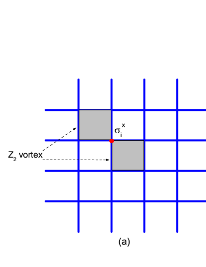
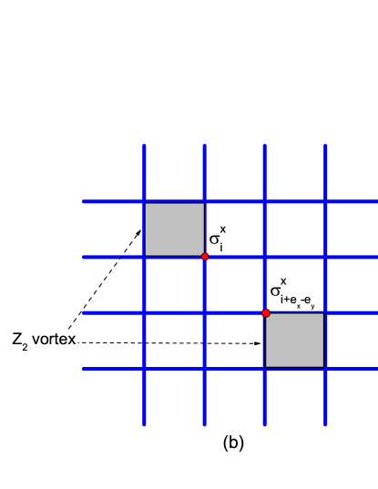
Figure 4: Generation and Hopping of $Z_{2}$ vortex. The shadow plaquettes represent $Z_{2}$ vortices.

From Eq.(25), one may obtain the energy splitting $\Delta E$ of the two ground states as

$$\delta E=U_{I}^{(L)}=\langle\uparrow\mid\hat{H_{I}}(\frac{1}{E_{0}-\hat{H}_{0}}\hat{H_{I}})^{L_{0}-1}\left|\downarrow\right\rangle.$$ (26)

Due to the translation invariance, to calculate $(\frac{1}{E_{0}-\hat{H}_{0}}\hat{H_{I}})\left|\downarrow\right\rangle=(\frac{h^{x}}{E_{0}-\hat{H}_{0}}\sum\limits_{i}\sigma_{i}^{x})\left|\downarrow\right\rangle,$ we can choose site $i$ as the starting point of the tunneling process and get

$$(\frac{1}{E_{0}-\hat{H}_{0}}\hat{H_{I}})\left|\downarrow\right\rangle \rightarrow L_{x}L_{y}(\frac{h^{x}}{E_{0}-\hat{H}_{0}}\sigma_{i}^{x})\left|\downarrow\right\rangle$$

$$= L_{x}L_{y}(\frac{h^{x}}{E_{0}-\hat{H}_{0}})\left|\Psi_{i}\right\rangle$$

where $\left|\Psi_{i}\right\rangle$ is the excited state of two $Z_{2}$ vortices (or $Z_{2}$ charges) at plaquettes $i-e_{y}$ and $i-e_{x}$ with an energy $E_{0}+4g$ (See Fig.4(a)). From $\hat{H}_{0}\left|\Psi_{i}\right\rangle=(E_{0}+4g)\left|\Psi_{i}\right\rangle,$ we have

$$(\frac{1}{E_{0}-\hat{H}_{0}}\hat{H_{I}})\left|\downarrow\right\rangle=L_{x}L_{y}(\frac{h^{x}}{-4g})\left|\Psi_{i}\right\rangle.$$

In next step, one $Z_{2}$ vortex (or $Z_{2}$ charge) moves one step, we get

$$(\frac{h^{x}}{E_{0}-\hat{H}_{0}}\sum\limits_{i}\sigma_{i}^{x})^{2}\left|\downarrow\right\rangle$$ (28)

$$= (\frac{h^{x}}{E_{0}-\hat{H}_{0}}\sum\limits_{i}\sigma_{i}^{x})L_{x}L_{y}(\frac{h^{x}}{-4g})\left|\Psi_{i}\right\rangle$$

$$= L_{x}L_{y}(\frac{h^{x}}{-4g})(\frac{h^{x}}{E_{0}-\hat{H}_{0}}\sum\limits_{i}\sigma_{i}^{x})\left|\Psi_{i}\right\rangle$$

$$= L_{x}L_{y}(\frac{h^{x}}{-4g})(\frac{h^{x}}{E_{0}-\hat{H}_{0}}\sigma_{i+e_{x}-e_{y}}^{x})\left|\Psi_{i}\right\rangle$$

$$= L_{x}L_{y}(\frac{h^{x}}{-4g})(\frac{h^{x}}{-4g})\left|\Psi_{i}^{\prime}\right\rangle.$$

where $\left|\Psi_{i}^{\prime}\right\rangle$ is the excited state of two $Z_{2}$ vortices (or $Z_{2}$ charges) at plaquettes $i+e_{x}-2e_{y}$ and $i-e_{x}$. See Fig.4(b). Then step by step, one $Z_{2}$ vortex (or $Z_{2}$ charge) moves around the torus. When the $Z_{2}$ vortex (or $Z_{2}$ charge) goes back to its starting point and annihilates with the other, the original quantum state $\left|\downarrow\right\rangle$ changes into $\mid\uparrow\rangle$. Finally we get the energy splitting

$$\Delta = 2\delta E=2U_{I}^{(L)}=2\langle\uparrow\mid\hat{H_{I}}(\frac{1}{E_{0}-\hat{H}_{0}}\hat{H_{I}})^{L_{0}-1}\left|\downarrow\right\rangle$$ (29)

$$= 2\times L_{x}L_{y}\frac{(h^{x})^{L_{0}}}{(-4g)^{L_{0}-1}}=8L_{x}L_{y}g(\frac{h^{x}}{4g})^{L_{0}}.$$

It is noted that $L_{0}-1$ is an even number.

Because the quantum tunneling process of $Z_{2}$ vortex (or $Z_{2}$ charge) plays a role of $\tau^{x}$ on the quantum states $\left(\begin{array}[]{c}\mid\uparrow\rangle\\ \mid\downarrow\rangle\end{array}\right)$ as

$$\left(\begin{array}[]{c}\mid\downarrow\rangle\\ \mid\uparrow\rangle\end{array}\right)=\tau^{x}\left(\begin{array}[]{c}\mid\uparrow\rangle\\ \mid\downarrow\rangle\end{array}\right),$$ (30)

we obtain the effective pseudo-spin Hamiltonian due to the contribution of $Z_{2}$ vortex (or $Z_{2}$ charges) as

$$\mathcal{\hat{H}}_{\mathrm{eff}}=\frac{\Delta}{2}(\mid\uparrow\rangle\langle\downarrow\mid+\mid\downarrow\rangle\langle\uparrow\mid)=J_{x}\tau^{x}$$ (31)

where $J_{x}=\Delta/2$ kou1 ; kou1' .

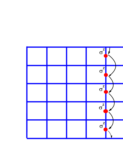
Figure 5: Tunneling path of virtual fermion along $\hat{e}_{y}$-direction on an $5\times 5$ lattice (The dots on the links denote the fermions).

For the second tunneling process, a virtual fermion will move around the torus along direction $\hat{e}_{y}$ with length $L_{y}$ (It is noted that due to $L_{x}\geq L_{y},$ the length of tunneling path along $\hat{e}_{x}$ direction is longer). See Fig.5. Such a tunneling process changes the quantum states $\left(\begin{array}[]{c}\mid\uparrow\rangle\\ \mid\downarrow\rangle\end{array}\right)$ turn into $\left(\begin{array}[]{c}\mid\uparrow\rangle\\ -\mid\downarrow\rangle\end{array}\right)=\tau^{z}\left(\begin{array}[]{c}\mid\uparrow\rangle\\ \mid\downarrow\rangle\end{array}\right)$. The extra sign of the state $\mid\downarrow\rangle$ comes from the presence of $\pi$ flux of fermionic quasi-particles through the holes of the torus. From Eq.25, we can get the energy shift of the state $\mid\downarrow\rangle$ as

$$\delta E=\sum\limits_{j=0}^{\infty}\langle\downarrow\mid\hat{H}_{I}(\frac{1}{E_{0}-\hat{H}_{0}}\hat{H}_{I})^{j}\mid\downarrow\rangle=L_{x}L_{y}\frac{(h^{z})^{L_{y}}}{(8g)^{L_{y}-1}}$$ (32)

with an even number $L_{y}-1$. Through the same approach, we get the energy shift $\Delta E$ of $\mid\downarrow\rangle$ is equal to $-L_{x}L_{y}\frac{(h^{z})^{L_{y}}}{(8g)^{L_{y}-1}}.$ Then an energy difference $\varepsilon$ of the two ground states is obtained as

$$\varepsilon=2\delta E=16L_{x}L_{y}g(\frac{h^{z}}{8g})^{L_{y}}.$$ (33)

Finally the two-level quantum system of the two degenerate ground states on an $o\ast o$ lattice can be described by a simple effective pseudo-spin Hamiltonian

$$\mathcal{\hat{H}}_{\mathrm{eff}} = \frac{\Delta}{2}(\mid\uparrow\rangle\langle\downarrow\mid+\mid\downarrow\rangle\langle\uparrow\mid)+\frac{\varepsilon}{2}(\mid\uparrow\rangle\langle\uparrow\mid-\mid\downarrow\rangle\langle\downarrow\mid)$$

$$= J_{x}\tau^{x}+J_{z}\tau^{z}$$

where $J_{x}=\Delta/2$ and $J_{z}=\varepsilon/2$. By diagonalizing the effective Hamiltonian matrix, we can get the eigenvalues of the two ground states

$$E_{\pm}=\pm\sqrt{(\frac{\Delta}{2})^{2}+(\frac{\varepsilon}{2})^{2}}.$$ (35)

The total energy splitting becomes

$$\Delta E=E_{+}-E_{-}=2\sqrt{(\frac{\Delta}{2})^{2}+(\frac{\varepsilon}{2})^{2}}.$$ (36)

For the Wen-plaquette model under external field along $x$-direction, the total energy splitting $\Delta E$ is reduced into $\Delta=8L_{x}L_{y}g(\frac{h^{x}}{4g})^{L_{0}}.$ On the other hand, for the Wen-plaquette model under external field along $z$-direction, the total energy splitting $\Delta E$ is $\varepsilon=16L_{x}L_{y}g(\frac{h^{z}}{8g})^{L_{y}}.$

IV.3 Macroscopic quantum tunneling effect of the degenerate ground states on $e\ast o$ lattice

Secondly, we study the MQT of the two degenerate ground states on an $L_{x}\times L_{y}$ ($L_{x}$ is an even number and $L_{y}$ is an odd number) lattice oe . Now we map the two-fold degenerate ground states $\mid m_{1}=0\rangle$ and $\mid m_{1}=1\rangle$ onto quantum states of the pseudo-spin $\mathbf{\hat{\tau}}_{1}$ as $\mid\uparrow\rangle_{1}$ and $\left|\downarrow\right\rangle_{1}$, respectively. Under the perturbation, $\hat{H}_{I}=h^{x}\sum\limits_{i}\sigma_{i}^{x}+h^{z}\sum\limits_{i}\sigma_{i}^{z}$, there are two types of quantum tunneling processes - virtual $Z_{2}$-vortex (or $Z_{2}$ charge) propagating along $\hat{e}_{x}-\hat{e}_{y}$ directions around the torus and virtual fermion propagating along $\hat{e}_{y}$ direction around the torus.

For the virtual $Z_{2}$-vortex (or $Z_{2}$ charge) propagating along $\hat{e}_{x}-\hat{e}_{y}$ directions around the torus, the energy splitting $\Delta$ can be obtained by the high-order degenerate-state perturbation theory as

$$\Delta = 2\langle\uparrow\mid_{1}\hat{H_{I}}(\frac{1}{E_{0}-\hat{H}_{0}}\hat{H_{I}})^{L_{0}-1}\left|\downarrow\right\rangle_{1}$$

$$= 2L_{x}L_{y}\frac{(h^{x})^{L_{0}}}{(-4g)^{L_{0}-1}}.$$

Because the quantum tunneling process of $Z_{2}$ vortex (or $Z_{2}$ charge) plays a role of $\tau_{1}^{x}$ on the quantum states $\left(\begin{array}[]{c}\mid\uparrow\rangle_{1}\\ \mid\downarrow\rangle_{1}\end{array}\right)$ as $\left(\begin{array}[]{c}\mid\downarrow\rangle_{1}\\ \mid\uparrow\rangle_{1}\end{array}\right)=\tau_{1}^{x}\left(\begin{array}[]{c}\mid\uparrow\rangle_{1}\\ \mid\downarrow\rangle_{1}\end{array}\right),$ we obtain the effective pseudo-spin Hamiltonian due to the contribution of $Z_{2}$ vortex (or $Z_{2}$ charge) as

$$\mathcal{\hat{H}}_{\mathrm{eff}}=\frac{\Delta}{2}(\mid\uparrow\rangle_{1}\langle\downarrow\mid_{1}+\mid\downarrow\rangle_{1}\langle\uparrow\mid_{1})=J_{x}\tau_{1}^{x}$$ (38)

where $J_{x}=\Delta/2$.

For the tunneling process of fermion propagating around the torus along direction $\hat{e}_{y}$, we obtain the energy difference $\varepsilon$ of the two ground states as

$$\varepsilon=2\Delta E=16L_{x}L_{y}g(\frac{h^{z}}{8g})^{L_{y}}.$$ (39)

The length of the tunneling path is $L_{y}$ which is an odd number. Such tunneling process plays a role of $\tau_{1}^{z}$.

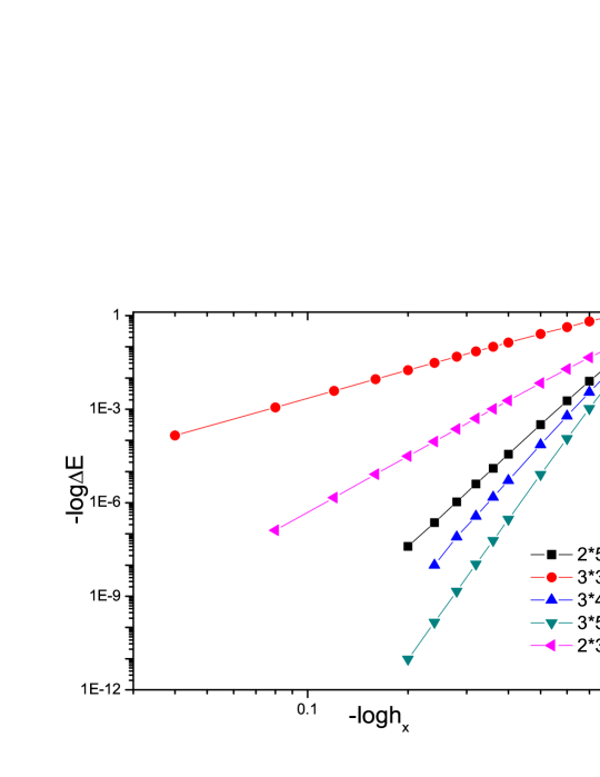
Figure 6: The energy splitting between the two degenerate ground states of the Wen-plaquette model in an external field along $x$-direction ($g=1$). Here $N\ast M$ denotes a $N\times M$ lattice.

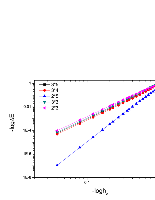
Figure 7: The energy splitting between the two degenerate ground states of the Wen-plaquette model in an external field along $z$-direction ($g=1$). Here $N*M$ denotes a $N\times M$ lattice.

Finally the two-level quantum system of the two degenerate ground states on an $e\ast o$ lattice can be described by

$$\mathcal{\hat{H}}_{\mathrm{eff}}=J_{x}\tau_{1}^{x}+J_{z}\tau_{1}^{z}$$ (40)

where $J_{x}=\Delta/2$ and $J_{z}=\varepsilon/2$. The total energy splitting now becomes

$$\Delta E=E_{+}-E_{-}=2\sqrt{(\frac{\Delta}{2})^{2}+(\frac{\varepsilon}{2})^{2}}.$$ (41)

In Fig.6 and Fig.7, we plot the numerical results from the exact diagonalization technique of the Wen-plaquette model on different $o\ast o$ and $e\ast o$ lattices. Table.(IV) shows the tunneling lengths $L_{0}$ from the numerical results (the numbers in the brackets are the theoretical predictions), which indicate that our theoretical results are consistent with the numerical results from exact diagonalization approach.

$L_{0}$	$3\ast 3$	$2\ast 5$	$3\ast 4$	$3\ast 5$
$h_{x}$	2.98312 (3)	9.84653 (10)	12.10754 (12)	15.01707 (15)
$h_{z}$	3.06994 (3)	4.83737 (5)	3.03164 (3)	3.01557 (3)

Table 4: The tunneling lengths $L_{0}$ from the numerical results (the numbers in the brackets are the theoretical predictions). $h_{x}$ means the external field along $x$-direction and $h_{z}$ means the external field along $z$-direction. Here $N*M$ denotes a $N\times M$ lattice.

IV.4 Macroscopic quantum tunneling effect of the degenerate ground states on $e\ast e$ lattice

Thirdly, we study the MQT of the four degenerate ground states on an $L_{x}\times L_{y}$ ($L_{x}$ and $L_{y}$ are even numbers with $L_{x}\geq L_{y}$) lattice. We denote the four degenerate ground states $\mid m_{1},m_{2}\rangle=$ $|0,0\rangle,$ $|1,0\rangle,$ $|0,1\rangle,$ $|1,1\rangle$ by the quantum states of pseudo-spin $\mathbf{\hat{\tau}}_{1\text{ }}$and $\mathbf{\hat{\tau}}_{2}$. Under the perturbation, $\hat{H}_{I}=h^{x}\sum\limits_{i}\sigma_{i}^{x}+h^{z}\sum\limits_{i}\sigma_{i}^{z}$, there are five types of quantum tunneling processes - virtual $Z_{2}$-vortex propagating along $\hat{e}_{x}-\hat{e}_{y}$ direction around the torus, $Z_{2}$ charge propagating along $\hat{e}_{x}-\hat{e}_{y}$ direction around the torus, and virtual fermion propagating along $\hat{e}_{x},$ $\hat{e}_{y},$ $\hat{e}_{x}-\hat{e}_{y}$ direction around the torus, respectively. We will calculate the ground state energy splitting from the degenerate perturbation approach one by one.

In the first step we study the quantum tunneling process of $Z_{2}$-vortex propagating along $\hat{e}_{x}-\hat{e}_{y}$ direction around the torus. After such tunneling process, the quantum states $\left(\begin{array}[]{c}\mid 0,0\rangle\\ \mid 1,0\rangle\\ \mid 0,1\rangle\\ \mid 1,1\rangle\end{array}\right)$ turn into

$$\left(\begin{array}[]{c}\mid 0,0\rangle\\ \mid 1,0\rangle\\ \mid 0,1\rangle\\ \mid 1,1\rangle\end{array}\right)\rightarrow\left(\begin{array}[]{c}\mid 1,1\rangle\\ \mid 0,1\rangle\\ \mid 1,0\rangle\\ \mid 0,0\rangle\end{array}\right)=\tau_{1}^{x}\mathbf{\otimes}\tau_{2}^{x}\left(\begin{array}[]{c}\mid 0,0\rangle\\ \mid 1,0\rangle\\ \mid 0,1\rangle\\ \mid 1,1\rangle\end{array}\right).$$ (42)

Thus we may use the pseudo-spin operator $\tau_{1}^{x}\mathbf{\otimes}\tau_{2}^{x}$ to denote the tunneling process. The effective pseudo-spin Hamiltonian due to the contribution of $Z_{2}$ vortex is obtained as

$$\mathcal{\hat{H}}_{\mathrm{eff}}=J_{xx}\tau_{1}^{x}\mathbf{\otimes}\tau_{2}^{x}$$ (43)

where $J_{xx}=L_{x}L_{y}\frac{(h^{x})^{L_{0}}}{(-4g)^{L_{0}-1}}.$ Similar to the results in above section, the length $L_{0}$ of the tunneling path is equal to $\frac{L_{x}L_{y}}{\xi}$ where $\xi$ is the maximum common divisor for $L_{x}$ and $L_{y}$.

In the second step we study the quantum tunneling process of $Z_{2}$-charge propagating along $\hat{e}_{x}-\hat{e}_{y}$ directions around the torus. We may use the pseudo-spin operator $\tau_{1}^{y}\mathbf{\otimes}\tau_{2}^{y}$ to denote this tunneling process, of which the effective pseudo-spin Hamiltonian is obtained as

$$\mathcal{\hat{H}}_{\mathrm{eff}}=J_{yy}\tau_{1}^{y}\mathbf{\otimes}\tau_{2}^{y}$$ (44)

where $J_{yy}=L_{x}L_{y}\frac{(h^{x})^{L_{0}}}{(-4g)^{L_{0}-1}}$ and $L_{0}=\frac{L_{x}L_{y}}{\xi}.$

In the third step we study the quantum tunneling process of fermion propagating along $\hat{e}_{x}$ and $\hat{e}_{y}$ directions around the torus, of which the pseudo-spin operators correspond to $\mathbf{1}\otimes\tau_{2}^{z}$ and $\tau_{1}^{z}\otimes\mathbf{1}$, respectively. Then the effective pseudo-spin Hamiltonian due to the contribution of the two quantum tunneling processes is obtained as

$$\mathcal{\hat{H}}_{\mathrm{eff}}=\tilde{h}_{1}^{z}\left(\tau_{1}^{z}\mathbf{\otimes 1}\right)+\tilde{h}_{2}^{z}\left(\mathbf{1\otimes}\tau_{2}^{z}\right)$$ (45)

where $\tilde{h}_{1}^{z}=-8L_{x}L_{y}g(\frac{h^{z}}{8g})^{L_{x}}\$and $\tilde{h}_{2}^{z}=-8L_{x}L_{y}g(\frac{h^{z}}{8g})^{L_{y}}$.

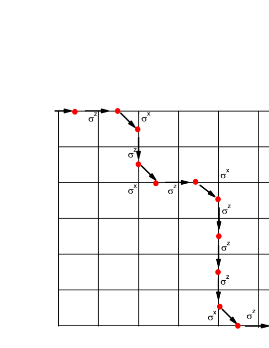
Figure 8: Tunneling path of virtual fermions on an $6\times 6$ lattice with 4 corners (The dots on the links denotes fermions).

In the last step we study the quantum tunneling process of fermion propagating along $\hat{e}_{x}-\hat{e}_{y}$ direction around the torus, of which the pseudo-spin operator corresponds to $\tau_{1}^{z}\mathbf{\otimes}\tau_{2}^{z}$, respectively. Now there are a lot of tunneling pathes with same length $2L_{0}$. Different tunneling pathes can be labeled by the positions of corners, at which the fermions make a turn round from vertical links to parallel links (or parallel links to vertical links). For a path with $2k$ corners ($k$ is an positive integer number), the topological closed string operator can be written as

$$W_{f}(\mathcal{C}_{XY})=\sigma_{i}^{z}\sigma_{i+1}^{z}...\sigma_{j-1}^{z}\sigma_{j}^{x}\sigma_{j+1}^{z}...\sigma_{2L_{0}-2}^{x}\sigma_{2L_{0}-1}^{z}\sigma_{2L_{0}}^{z}$$ (46)

with the site $i=(i_{x},i_{y})$ and a neighboring site $i+1$. See Fig.8. Along the closed loops, each operator $\sigma_{j}^{x}$ corresponds to a corner. Therefore, the number of pathes with $2k$ corners that is equal to the power of $h^{x}$ in $\Delta E$ is obtained as

$$C_{L_{0}-1}^{k}=\frac{\left(L_{0}-1\right)!}{k!(L_{0}-k-1)!}.$$ (47)

It is noted that for any path, there are at least two corners. Then after considering the tunneling processes of all possible pathes, the matrix element of $\tau_{1}^{z}\mathbf{\otimes}\tau_{2}^{z}$ is obtained as

$$J_{zz} = \varepsilon=L_{x}L_{y}C_{L_{0}-1}^{1}\frac{(2h^{x})^{2}(h^{z})^{2L_{0}-2}}{(-8g)^{2L_{0}-1}}$$

$$+L_{x}L_{y}C_{L_{0}-1}^{2}\frac{(2h^{x})^{4}(h^{z})^{2L_{0}-4}}{(-8g)^{2L_{0}-1}}+...$$

$$+L_{x}L_{y}C_{L_{0}-1}^{k}\frac{(2h^{x})^{2k}(h^{z})^{2L_{0}-2k}}{(-8g)^{2L_{0}-1}}$$

$$+...+L_{x}L_{y}\frac{(2h^{x})^{2L_{0}}}{(-8g)^{2L_{0}-1}}$$

$$= -L_{x}L_{y}\frac{[(2h^{x})^{2}+(h^{z})^{2}]^{L_{0}}-(h^{z})^{2L_{0}}}{(8g)^{2L_{0}-1}}.$$

Finally we derive an effective pseudo-spin Hamiltonian of the four ground states as

$$\mathcal{\hat{H}}_{\mathrm{eff}}\simeq J_{xx}\left(\tau_{1}^{x}\mathbf{\otimes}\tau_{2}^{x}\right)+J_{yy}\left(\tau_{1}^{y}\mathbf{\otimes}\tau_{2}^{y}\right)+J_{zz}\left(\tau_{1}^{z}\mathbf{\otimes}\tau_{2}^{z}\right)+\tilde{h}_{1}^{z}\left(\tau_{1}^{z}\mathbf{\otimes 1}\right)+\tilde{h}_{2}^{z}\left(\mathbf{1\otimes}\tau_{2}^{z}\right)$$

which is equal to

$$\mathcal{\hat{H}}_{\mathrm{eff}}=\left(\begin{array}[]{cccc}J_{zz}+\widetilde{h_{1}^{z}}+\widetilde{h_{2}^{z}}&0&0&J_{xx}-J_{yy}\\ 0&-J_{zz}+\widetilde{h_{1}^{z}}-\widetilde{h_{2}^{z}}&J_{xx}+J_{yy}&0\\ 0&J_{xx}+J_{yy}&-J_{zz}-\widetilde{h_{1}^{z}}+\widetilde{h_{2}^{z}}&0\\ J_{xx}-J_{yy}&0&0&J_{zz}-\widetilde{h_{1}^{z}}-\widetilde{h_{2}^{z}}\end{array}\right).$$ (49)

The coefficients of $\mathcal{\hat{H}}_{\mathrm{eff}}$ are given by

$$J_{xx} = J_{yy}=L_{x}L_{y}\frac{(h^{x})^{L_{0}}}{(-4g)^{L_{0}-1}},$$ (50)

$$J_{zz} = -L_{x}L_{y}\frac{[(2h^{x})^{2}+(h^{z})^{2}]^{L_{0}}-(h^{z})^{2L_{0}}}{(8g)^{2L_{0}-1}},$$

$$\tilde{h}_{1}^{z} = -8L_{x}L_{y}g(\frac{h^{z}}{8g})^{L_{x}},\text{ }\tilde{h}_{2}^{z}=-8L_{x}L_{y}g(\frac{h^{z}}{8g})^{L_{y}}.$$

By diagonalizing the effective Hamiltonian, we get the energies of the ground states as

$$E_{1} = J_{zz}-\sqrt{(\tilde{h}_{1}^{z}-\tilde{h}_{2}^{z})^{2}+4J_{xx}^{2}},$$ (51)

$$E_{2} = J_{zz}+\sqrt{(\tilde{h}_{1}^{z}-\tilde{h}_{2}^{z})^{2}+4J_{xx}^{2}},$$

$$E_{3} = J_{zz}+\tilde{h}_{1}^{z}+\tilde{h}_{2}^{z},$$

$$E_{4} = J_{zz}-\tilde{h}_{1}^{z}-\tilde{h}_{2}^{z}.$$

Because the parameter $J_{zz}$ is always much smaller than others as $\left|J_{zz}\right|\ll\left|J_{xx}\right|,$ $\left|J_{yy}\right|,$ $\left|\tilde{h}_{1}^{z}\right|,$ $\left|\tilde{h}_{2}^{z}\right|$, we may simplify $\mathcal{\hat{H}}_{\mathrm{eff}}$ askou1

$$\mathcal{\hat{H}}_{\mathrm{eff}}\simeq J_{xx}\left(\tau_{1}^{x}\mathbf{\otimes}\tau_{2}^{x}\right)+J_{yy}\left(\tau_{1}^{y}\mathbf{\otimes}\tau_{2}^{y}\right)+\tilde{h}_{1}^{z}\left(\tau_{1}^{z}\mathbf{\otimes 1}\right)+\tilde{h}_{2}^{z}\left(\mathbf{1\otimes}\tau_{2}^{z}\right)$$ (52)

and obtain the energies as

$$E_{1} \simeq -\sqrt{(\tilde{h}_{1}^{z}-\tilde{h}_{2}^{z})^{2}+4J_{xx}^{2}},$$ (53)

$$E_{2} \simeq \sqrt{(\tilde{h}_{1}^{z}-\tilde{h}_{2}^{z})^{2}+4J_{xx}^{2}},$$

$$E_{3} \simeq \tilde{h}_{1}^{z}+\tilde{h}_{2}^{z},$$

$$E_{4} \simeq -\tilde{h}_{1}^{z}-\tilde{h}_{2}^{z}.$$

Then when the external field increases ($h^{x}\neq 0$ and $h^{z}\neq 0$), the single energy level of the initial four degenerate ground states split into four energy levels.

If we apply the external field along $z$-direction, the four energy levels are

$$E_{1} \simeq -\tilde{h}_{1}^{z}+\tilde{h}_{2}^{z},\text{ }E_{2}\simeq\tilde{h}_{1}^{z}-\tilde{h}_{2}^{z},$$ (54)

$$E_{3} \simeq \tilde{h}_{1}^{z}+\tilde{h}_{2}^{z},\text{ }E_{4}\simeq-\tilde{h}_{1}^{z}-\tilde{h}_{2}^{z},$$

where $\tilde{h}_{1}^{z}=-8L_{x}L_{y}g(\frac{h^{z}}{8g})^{L_{x}}$ and $\tilde{h}_{2}^{z}=-8L_{x}L_{y}g(\frac{h^{z}}{8g})^{L_{y}}.$ In the anisotropic limit, $L_{x}\gg L_{y}$, we have $\left|\tilde{h}_{1}^{z}\right|\ll\left|\tilde{h}_{2}^{z}\right|$. In this case, the initial four degenerate ground states split into two groups, $E_{1}\simeq\tilde{h}_{2}^{z},$ $E_{2}\simeq-\tilde{h}_{2}^{z},$ $E_{3}\simeq\tilde{h}_{2}^{z}$ and $E_{4}\simeq-\tilde{h}_{2}^{z}.$ In each group, there are two energy levels, of which the energy splitting $E_{1}-E_{3}=2\tilde{h}_{1}^{z}$ is very tiny. In contrast, the energy ”gap” between the two groups $E_{1}-E_{2}=-2\tilde{h}_{2}^{z}$ is larger. One can see the energy levels of the Wen-plaquette model in external field along $z$-direction on $2\times 6$ lattice ($g=1$) in Fig.9. In the isotropic case, $L_{x}=L_{y}$, we have $\tilde{h}_{1}^{z}=\tilde{h}_{2}^{z}$. In this case, the initial four degenerate ground states split into $E_{1}=E_{2}=0$, $E_{3}=2\tilde{h}_{1}^{z}$ and $E_{4}=-2\tilde{h}_{1}^{z}.$ One can see the energy levels of the Wen-plaquette model in external field along $z$-direction on $4\times 4$ lattice ($g=1$) in Fig.10.

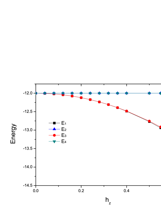
Figure 9: The ground state energies of the Wen-plaquette model in an external field along $z$-direction on $2\times 6$ lattice ($g=1$).

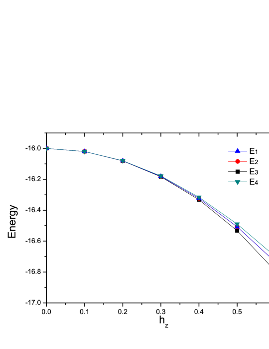
Figure 10: The ground state energies of the Wen-plaquette model in an external field along $z$-direction on $4\times 4$ lattice ($g=1$).

On the other hand, if we apply the external field along $x$-direction, the four energy levels become

$$E_{1} \simeq -2J_{xx},\text{ }E_{2}\simeq 2J_{xx},$$ (55)

$$E_{3} = E_{4}=J_{zz}\simeq 0,$$

where $J_{xx}=L_{x}L_{y}\frac{(h^{x})^{L_{0}}}{(-4g)^{L_{0}-1}}$ and $J_{zz}=-8L_{x}L_{y}g(\frac{h^{x}}{8g})^{2L_{0}}$. Now the initial four degenerate ground states split into three energy levels. One can see the energy levels of the Wen-plaquette model in an external field along $x$-direction on $4\times 4$ lattice ($g=1$) in Fig.11.

Figure 11: The ground state energies of the Wen-plaquette model in an external field along $x$-direction on $4\times 4$ lattice ($g=1$).

In addition, one may consider the MQT under a more general perturbation

$$\hat{H}_{I}=h^{x}\sum\limits_{i}\sigma_{i}^{x}+h^{y}\sum\limits_{i}\sigma_{i}^{y}+h^{z}\sum\limits_{i}\sigma_{i}^{z}.$$ (56)

For an external field of $h^{x}\neq 0,$ $h^{y}\neq 0$ and $h^{z}\neq 0,$ all quasi-particles ($Z_{2}$ vortex, $Z_{2}$ charge and fermion) can move along $\hat{e}_{x},$ $\hat{e}_{y},$ $\hat{e}_{x}\pm\hat{e}_{y}$ directions freely. Therefore, to calculate the MQT of the degenerate ground states on an $e\ast e$ lattice, all nine types of quantum tunneling processes should be considered. The corresponding effective pseudo-spin Hamiltonian of the four ground states turns into

$$\mathcal{H}_{\mathrm{eff}} = J_{xx}\left(\tau_{1}^{x}\mathbf{\otimes}\tau_{2}^{x}\right)+J_{yy}\left(\tau_{1}^{y}\mathbf{\otimes}\tau_{2}^{y}\right)+J_{zz}\left(\tau_{1}^{z}\mathbf{\otimes}\tau_{2}^{z}\right)$$ (57)

$$+J_{zx}\left(\tau_{1}^{z}\mathbf{\otimes}\tau_{2}^{x}\right)+J_{xz}\left(\tau_{1}^{x}\mathbf{\otimes}\tau_{2}^{z}\right)+\tilde{h}_{1}^{x}\left(\tau_{1}^{x}\mathbf{\otimes 1}\right)$$

$$+\tilde{h}_{2}^{x}\left(\mathbf{1\otimes}\tau_{2}^{x}\right)+\tilde{h}_{1}^{z}\left(\tau_{1}^{z}\mathbf{\otimes 1}\right)+\tilde{h}_{2}^{z}\left(\mathbf{1\otimes}\tau_{2}^{z}\right)$$

where $J_{xx},$ $J_{yy}$, $J_{zz},$ $J_{zx}$, $J_{xz},$ $\tilde{h}_{1}^{x},$ $\tilde{h}_{2}^{x}$, $\tilde{h}_{1}^{z},$ $\tilde{h}_{2}^{z}$ are determined by the energy splitting of the degenerate ground states from the nine tunneling processes kou1 ; kou1' . This issue (the MQT of Eq. (56)) will be studied elsewhere.

V Conclusion

In this paper, we study macroscopic quantum tunneling (MQT) effect of $Z_{2}$ topological order in the Wen-Plaquette model that is characterized by the quantum tunneling processes of different virtual quasi-particles moving around the torus. By focusing on the degenerate ground states, we get their effective pseudo-spin models. The coefficients of these effective pseudo-spin models are obtained by a high-order degenerate perturbation approach. With the help of the effective pseudo-spin models, the energies of the ground states are calculated and the results are consistent with those from exact diagnalization numerical technique.

In the future, the approach will be applied onto the MQTs of $Z_{2}$ topological order in other models, such as the Kitaev toric-code mode and the Kitaev model on honeycomb lattice. After learning the nature of the MQT of $Z_{2}$ topological orders in different models, one may know how to manipulate the degenerate ground states by controlling the external field and then do topological quantum computation within the degenerate ground states kou1 ; kou1' .

- (1) Mohsen Razavy, Quantum Theory of Tunneling, (World Scientific, 2003).
- (2) X. G. Wen, Quantum Field Theory of Many-Body Systems, (Oxford Univ. Press, Oxford, 2004).
- (3) X. G. Wen, Int. J. Mod. Phys. B 4, 239 (1990).
- (4) X. G. Wen, Phys. Rev. B 65, 165113 (2002).
- (5) X. G. Wen, Phys. Rev. D 68, 065003 (2003).
- (6) X. G. Wen, Phys. Rev. Lett. 90 (2), 016803 (2003).
- (7) A. Kitaev, Ann. Phys. 303, 2(2003).
- (8) A. Kitaev, Ann. Phys. 321, 2(2006).
- (9) L. B. Ioffe, et al., Nature 415, 503 (2002).
- (10) S. P. Kou, Phys. Rev. Lett. 102, 120402 (2009).
- (11) S. P. Kou, arXiv:quant-ph/0904.4165.
- (12) J. K. Pachos, Ann. Phys, 322, 1254 (2007).
- (13) C. W. Zhang, S. Tewari, and S. Das Sarma, Phys. Rev. Lett. 99, 220502 (2007). S. Tewari, et al., Phys. Rev. Lett. 98, 010506 (2007).
- (14) Y.-J. Han, R. Raussendorf, and L.-M. Duan, Phys. Rev. Lett. 98, 150404 (2007).
- (15) L. Jiang, et al., Nature Phys., doi:10.1038/nphys943 (2008) doi:10.1038/nphys943.
- (16) K.P. Schmidt, S. Dusuel, and J. Vidal, Phys. Rev. Lett. 100, 057208 (2008).
- (17) S. Dusuel, K.P. Schmidt, and J. Vidal, Phys. Rev. Lett. 100, 177204 (2008).
- (18) Chuanwei Zhang, et al., Proc. Natl. Acad. Sci. U.S.A. 104, 18415 (2007).
- (19) Chuanwei Zhang, S. L. Rolston, and S. Das Sarma, Phys. Rev. A 74, 042316 (2006). Chuanwei Zhang, V. W. Scarola, and S. Das Sarma, Phys. Rev. A 76, 023605 (2007).
- (20) C. Y. Lu, et al., Phys. Rev. Lett. 102, 030502 (2009).
- (21) J. Vidal, S. Dusuel, and K.P. Schmidt, Phys. Rev. B 79, 033109 (2009).
- (22) J. Vidal, R. Thomale, K.P. Schmidt, and S. Dusuel, arXiv:0902.3547 (2009).
- (23) S. P. Kou, M. Levin, and X. G. Wen, Phys. Rev. B 78, 155134 (2008).
- (24) J. Yu, S. P. Kou and X. G. Wen, Eur. Puys. Letts, 84 17004, (2008).
- (25) The MQT on lattice is identical to that on lattice, except that the two degenerate states are denoted by rather than .