$F$-wave pairing of cold atoms in optical lattices

Abstract

The tremendous development of cold atom physics has opened up a whole new opportunity to study novel states of matter which are not easily accessible in solid state systems. Here we propose to realize the $f$-wave pairing superfluidity of spinless fermions in the $p_{x,y}$-orbital bands of the two dimensional honeycomb optical lattices. The non-trivial orbital band structure rather than strong correlation effects gives rise to the unconventional pairing with the nodal lines of the $f$-wave symmetry. With a confining harmonic trap, zero energy Andreev bound states appear around the circular boundary with a six-fold symmetry. The experimental realization and detection of this novel pairing state are feasible.

I Introduction

The study of unconventional Cooper pairing states has been a major subject in condensed matter physics for decades. In addition to the isotropic $s$-wave pairing, many unconventional pairing states have been identified sigrist1991 . For example, different types of $p$-wave pairing states were found in the superfluid ³He systems leggett1975 ; osheroff1997 including the anisotropic chiral $A$-phase and the isotropic $B$-phase. Evidence of the $p$-wave paring was also found in the ruthenate compound of Sr₂RuO₄ nelson2004 ; kidwingira2006 . The $d$-wave pairing states are most convincingly proved in the high-$T_{c}$ cuprates with phase sensitive measurements including Josephson tunneling junction harlingen1995 ; tsuei2000 and zero energy Andreev bound states hu1994 ; deutscher2005 . Many heavy fermion compounds exhibit evidence of unconventional Cooper pairing such as UPt₃, UBe₁₃, and CeCoIn₅ with nodal points or lines joynt2002 ; maclaughlin1984 ; izawa2001 ; strand2009 . However, conclusive experimental evidence to determine pairing symmetries is still lacking. These unconventional pairing states are driven by strong correlation effects, which brings significant difficulties for theoretical analysis and prediction. It would be great to find novel unconventional pairing mechanisms easier to handle.

On the other hand, cold atom physics has recently become an emerging frontier for condensed matter physics dalfovo1999 ; leggett2004 ; bloch2008 ; giorgini2008 . In particular, the $s$-wave pairing superfluidity of fermions through the Feshbach resonances has become a major research focus. The Bose-Einstein condensation (BEC) and Bardeen-Cooper-Schrieffer (BCS) crossover has been extensively investigated chin2008 ; chin2004 ; regal2004 ; zwierlein2004 ; partridge2005 . Naturally, searching for unconventional Cooper pairing states in cold atom systems is expected to stimulate more exciting physics. For example, the $p$-wave pairing states have been proposed by using the $p$-wave Feshbach resonances ho2005 ; gurarie2007 ; cheng2005 , which, however, suffer from a drawback of heavy particle loss. The unconventional Cooper pairing states with cold atoms have not been realized yet zhang2004 ; gaebler2007 ; fuchs2008 ; inada2008 .

In this article, we propose a novel $f$-wave pairing state of spinless fermions in the cold atom optical lattices. This unconventional pairing arises from the non-trivial band structure of the $p_{x,y}$-orbital bands in the honeycomb optical lattices combined with a conventional attractive interaction. The internal orbital configurations of the Bloch wave band eigenstates vary with the crystal momenta, resulting in an $f$-wave angular form factor for the pairing order parameters. Along three high symmetry lines in the Brillouin zone whose directions differ by 120^∘ from each other, the intra-band pairing order parameters are exactly suppressed to zero. The unconventional nature of this pairing exhibits in the appearance of the zero-energy Andreev bound states at the circular boundary with imposing a confining trap. Since no strong correlation effects are involved, our analysis below is well-controllable. This is a novel state of matter, which to our knowledge has not been unambiguously identified before neither in condensed matter nor in cold atom systems, thus this result will greatly enrich the study of unconventional pairing states.

This article is organized as follows. In Section II, we explain the orbital structure of the Bloch wave eigenstate in detail. In Section III, we show that the $f$-wave Cooper pairing naturally arises from a conventional on-site Hubbard attraction. In Section IV, we discuss the zero energy Andreev bound state at the edge of the confining trap, which provides a phase sensitive evidence. In Section V, we discuss the experiment realization and detection. Conclusions are given in Section VI.

II The orbital structure of the $p$-band Bloch wave functions

The honeycomb optical lattice was experimentally constructed quite some years ago by using three coplanar blue detuned laser beams whose wavevectors $\vec{k}_{i}~{}(i=1,2,3)$ differ by 120^∘ from each other grynberg1993 . After the lowest $s$-orbital band is fulfilled, the next active ones are $p_{x,y}$-orbital bands lying in the hexagonal plane. Different from the situation in graphene whose $p_{x,y}$-orbital bands strongly hybridize with the $s$-orbital bands and are pushed away from the Fermi surface, the hybridization between the $p_{x,y}$ and $s$-orbitals in the optical honeycomb lattice is negligible. The $p_{z}$-orbital band can be pushed to higher energies and thus unoccupied by imposing strong confinement along the $z$-axis. The $p_{x,y}$-orbital bands exhibit the characteristic features of orbital physics, i.e., spatial anisotropy and orbital degeneracy. This provides a new perspective of the honeycomb lattice, and is complementary to the research focusing on the $p_{z}$-band system of graphene which is not orbitally active. The novel physics which does not appear in graphene includes the flat band structurewu2007 , the consequential non-perturbative strong correlation effects (e.g. Wigner crystal wu2007a and ferromagnetismzhang2008 ), frustrations in orbital exchangewu2008 , and the quantum anomalous Hall effectwu2008a .

We employ the $p_{x,y}$-orbital band Hamiltonian studied in Ref. wu2007 ; wu2007a ; wu2008 ; wu2008a as

$$H_{0}=t_{\parallel}\sum_{\vec{r}\in A,i=1,2,3}\{p^{\dagger}_{\vec{r},i}p_{\vec{r}+a\vec{e}_{i},i}+{\rm h.c.}\}-\mu\sum_{\vec{r}\in A\oplus B}n_{\vec{r}},$$ (1)

where $\hat{e}_{1,2,3}$ are unit vectors from one site in sublattice $A$ to its three neighboring sites in sublattice $B$ defined as $\hat{e}_{1,2}=\pm\frac{\sqrt{3}}{2}\hat{e}_{x}+\frac{1}{2}\hat{e}_{y},\hat{e}_{3}=-\hat{e}_{y}$; $p_{i}\equiv(p_{x}\hat{e}_{x}+p_{y}\hat{e}_{y})\cdot\vec{e}_{i}$ is the $p$-orbital projected onto the bond along the direction of $\hat{e}_{i}$ and only two of them are linearly independent; $n_{\vec{r}}=n_{\vec{r},x}+n_{\vec{r},y}$ is the particle number at site $\vec{r}$; the $\sigma$-bonding $t_{\parallel}$ describes the hopping between $p$-orbitals on neighboring sites parallel to the bond direction and is rescaled to 1 below; $a$ is the nearest neighbor distance. $t_{\parallel}$ is positive due to the odd parity of $p$-orbitals. Eq. 1 neglects the $\pi$-bonding $t_{\perp}$ describing the hopping between $p$-orbitals perpendicular to the bond direction. Due to the high spatial anisotropy of the $p$-orbitals, $t_{\perp}/t_{\parallel}\ll 1$. To confirm this, we have fitted $t_{\perp}$ and $t_{\parallel}$ from a realistic band structure calculation for the sinusoidal optical potential

$$V(\vec{r})=V_{0}\sum_{1\leq i<j\leq 3}\cos\{(\vec{k}_{i}-\vec{k}_{j})\cdot\vec{r}\}.$$ (2)

With a moderate potential depth of $V_{0}/E_{R}=12$, $t_{\perp}/t_{\parallel}$ is already driven to $1\%$ with $t_{\parallel}\approx 0.375E_{R}$ where $E_{R}=\frac{\hbar^{2}k^{2}}{2M}$ is the recoil energy and $M$ is the atom mass. Further increasing $V_{0}/E_{R}$ decreases $t_{\perp}/t_{\parallel}$ even more.

Eq. 1 has a chiral symmetry, i.e., under the transformation of $p_{\vec{r},x(y)}\rightarrow-p_{\vec{r},x(y)}$ only for sites in sublattice A but not for sites in sublattice B, $H_{0}\rightarrow-H_{0}$. Thus its four bands have a symmetric spectra respect to the zero energy as

$$E_{1,4}=\mp\frac{3}{2}t_{\parallel},\,\,\,E_{2,3}=\mp\frac{t_{\parallel}}{2}\sqrt{3+2\sum_{i<j}\cos\vec{k}\cdot(\hat{e}_{i}-\hat{e}_{j})}.$$

The Brillouin zone (BZ) is a regular hexagon with the edge length $\frac{4\pi}{3\sqrt{3}a}$. Two middle dispersive bands $2$ and $3$ have two non-equivalent Dirac points $K(K^{\prime})=(\pm\frac{4\pi}{3\sqrt{3}a},0)$ with a band width of $\frac{3}{2}t_{\parallel}$. The bottom and top bands are flat. We define the four component annihilation operators in momentum space as $\hat{\phi}(\vec{k})=[\hat{p}_{A,x}(\vec{k}),\hat{p}_{A,y}(\vec{k}),\hat{p}_{B,x}(\vec{k}),\hat{p}_{B,y}(\vec{k})]^{T}$. In this basis, the eigen-operator $\hat{\psi}_{m}(\vec{k})$ for band $m$ can be diagonalized as $\hat{\psi}_{m}(\vec{k})=\hat{\phi}_{n}(\vec{k})U_{nm}(\vec{k})$ where $U(\vec{k})$ is a $4\times 4$ unitary matrix. The phase convention for band eigenvectors, i.e., each column of $U(\vec{k})$, is conveniently chosen as $R_{\frac{\pi}{3}}\hat{\psi}_{m}(\vec{k})R^{-1}_{\frac{\pi}{3}}=\,\mathrm{sgn}(m)\hat{\psi}_{m}(\vec{k}^{\prime})$ with $\,\mathrm{sgn}(m)=-$ for $m=1,2$ and $\,\mathrm{sgn}(m)=+$ for $m=3,4$, where the symmetry operation $R_{\frac{\pi}{3}}$ is the $60^{\circ}$ rotation around a center of the hexagonal plaquette and $\vec{k}^{\prime}=R_{\frac{\pi}{3}}\vec{k}$. The analytical form of $U_{nm}(\vec{k})$ is given in Appendix A.

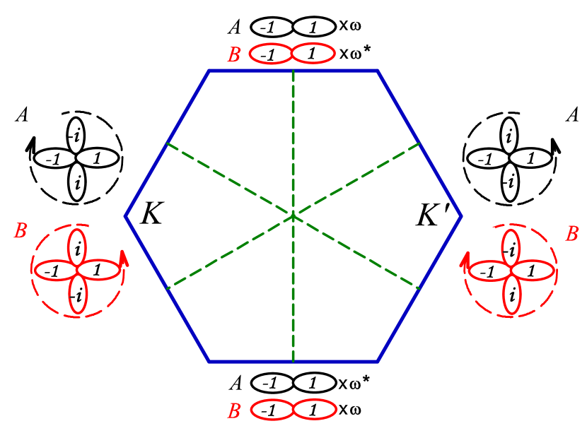
Figure 1: (Color online) Orbital configurations of the lower dispersive band 2 at high symmetry points and lines in the BZ. The time-reversal partners $\psi_{2}(\pm\vec{k})$ only involve the same polar orbital if $\vec{k}$ is along the three middle lines, and take the complex orthogonal orbitals of $p_{x}\pm ip_{y}$ with opposite chiralities at $\vec{K}$ and $\vec{K}^{\prime}$. $\omega=e^{i\frac{\pi}{6}}$.

The orbital configurations of the band eigenvectors have interesting patterns as depicted in Fig. 1, which arise from the lattice $D_{6h}$ symmetry. Only the lowest dispersive band ($m=2$) is plotted as an example. The lowest flat band ($m=1$) has the same symmetry structure except having different orbital polarization directions. The remaining two can be obtained by performing the operation of the chiral symmetry. Six lines in the BZ possess reflection symmetry, i.e., three passing the middle points of the opposite edges and three passing the opposite vertices of $\vec{K}$ and $\vec{K}^{\prime}$. The eigenvectors of each band along these lines should be either even or odd with respect to the corresponding reflection. For example, for the reflection respect to the $y$-axis, the orbitals transform as

$$\hat{p}_{A(B),x}\rightarrow-\hat{p}_{A(B),x},\ \ \ \hat{p}_{A(B),y}\rightarrow\hat{p}_{A(B),y},$$ (4)

thus the eigen-operators $\hat{\psi}_{m}(\vec{k})$ with $\vec{k}\parallel\hat{y}$ must be either purely $\hat{p}_{y}$ (even) or $\hat{p}_{x}$ (odd). For the other two middle lines, the corresponding eigenvectors are obtained by performing the $\pm 120^{\circ}$ rotation. For the time-reversal partners $\hat{\psi}_{m}(\vec{k})$ and $\hat{\psi}_{m}(-\vec{k})$ along these lines, they only take the same real polar orbitals. On the other hand, the reflection respect to the $x$-axis gives rise to the transformation

$$\hat{p}_{A(B),x}\rightarrow\hat{p}_{B(A),x},\ \ \,\hat{p}_{A(B),y}\rightarrow-\hat{p}_{B(A),y}.$$ (5)

Furthermore, $\vec{K}$ and $\vec{K}^{\prime}$ have three-fold rotational symmetry. Combining two facts together, $\hat{\psi}_{m}(\vec{K})$ should be of $p_{x}+ip_{y}$ for sites in one of the sublattices and $p_{x}-ip_{y}$ for sites in the other sublattice. Its time-reversal partner $\hat{\psi}_{m}(\vec{K}^{\prime})$ has the opposite chiralities in both sublattices respect to those at $\vec{K}$. In other words, the orbital configurations of $\hat{\psi}_{m}(\vec{k})$ are linear-polarized at the middle points of the BZ edge, changes to circularly-polarized at the vertices, and elliptically polarized in between.

III F-wave Cooper pairing

Next we introduce the on-site attractive interaction term between spinless fermions as

$$H_{int}=-U\sum_{\vec{r}}n_{\vec{r},x}n_{\vec{r},y},$$ (6)

where $U$ is positive. We perform the mean-field decomposition for $H_{int}$ in the pairing channel as

$$H^{pairing}_{int} = -\sum_{\vec{r}_{A,B}}\big{\{}\Delta^{*}_{A}p_{\vec{r}_{A},y}p_{\vec{r}_{A},x}+\Delta^{*}_{B}p_{\vec{r}_{B},y}p_{\vec{r}_{B},x}+h.c\big{\}},$$ (7)

$$= \sum^{\prime}_{\vec{k}}\sum_{m,n=1}^{4}\,\Delta^{*}_{nm}(\vec{k})\psi_{n}(\vec{k})\psi_{m}(-\vec{k})+h.c,$$

where the pairing order parameters in the $A$ and $B$-sublattices are self-consistently defined as $\Delta^{*}_{A(B)}=U\langle G|p^{\dagger}_{r_{A(B),x}}p^{\dagger}_{r_{A(B),y}}|G\rangle$; $\langle G|..|G\rangle$ means the average over the pairing ground state; the summation of $\vec{k}$ only covers half of the BZ; the multi-band pairing order parameters in momentum space has a $4\times 4$ matrix structure as

$$\Delta_{nm}(\vec{k})=U\langle G|\psi_{n}(\vec{k})\psi_{m}(-\vec{k})|G\rangle.$$ (8)

Under the rotation of $R_{\frac{\pi}{3}}$, it transforms as $R_{\frac{\pi}{3}}\Delta_{nm}(\vec{k})R_{\frac{\pi}{3}}^{-1}=\,\mathrm{sgn}(n)\,\mathrm{sgn}(m)\Delta_{nm}(\vec{k}^{\prime})$.

In addition, we also introduce the mean-field decomposition for $H_{int}$ in the charge-density-wave (CDW) channel as:

$$H^{CDW}_{int}=\sum_{\vec{r}_{A,B},\tau=x,y} (-U\,n-\frac{N}{2}) p^{\dagger}_{\vec{r}_{A},\tau}p_{\vec{r}_{A},\tau}$$

$$+ (-U\,n+\frac{N}{2}) p^{\dagger}_{\vec{r}_{B},\tau}p_{\vec{r}_{B},\tau},$$ (9)

where

$$n=\langle G|(n_{\vec{r}_{A},x}+n_{\vec{r}_{A},y}+n_{\vec{r}_{B},x}+n_{\vec{r}_{B},y})/2|G\rangle$$ (10)

is the total particle filling, and

$$N=U\langle G|(n_{\vec{r}_{A},x}+n_{\vec{r}_{A},y}-n_{\vec{r}_{B},x}-n_{\vec{r}_{B},y})|G\rangle$$ (11)

is the CDW order parameter. Generally speaking, the CDW becomes important in large $U$ or close to half-filling ($n=1$) as will be discussed below.

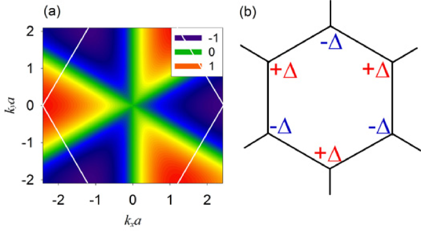
Figure 2: (Color online) A) The $f$-wave pairing form factor $F(\vec{k})$ for the intra-band pairing in momentum space. B) The $f$-wave pairing pattern in real space with $\Delta_{A}=-\Delta_{B}=\Delta$.

The intra-band gap functions $\Delta_{nn}$ can be calculated analytically as $\Delta_{nn}(\vec{k})=i(-)^{n}\frac{1}{2}(\Delta_{A}-\Delta_{B})F(\vec{k})$ with the $f$-wave form factor of

$$F(\vec{k})=\frac{16}{\sqrt{3}N_{0}(\vec{k})}\sin\frac{\sqrt{3}}{2}k_{x}\left[\cos\frac{\sqrt{3}}{2}k_{x}-\cos\frac{3}{2}k_{y}\right],$$ (12)

where $N_{0}$ satisfies

$$N_{0}(\vec{k})=\frac{8}{3}\big{\{}3-\sum_{1\leq i<j\leq 3}\cos\vec{k}\cdot(\hat{e}_{i}-\hat{e}_{j})\big{\}}.$$ (13)

$\Delta_{A}$ can be fixed positive, and $\Delta_{B}=|\Delta_{B}|e^{i\Delta\theta}$ with a relative phase $\Delta\theta$. The optimal $\Delta\theta$ takes the value of $\pi$, i.e., $\Delta_{A}=-\Delta_{B}$, to maximize the intra-band pairings. We have confirmed this in the explicit self-consistent mean-field solution for Eq. 1 and Eq. 7. Furthermore, the non-vanishing $\pi$-bonding $t_{\perp}$ term can further stabilize this solution as a result of the odd parity of $\pi$-orbitals.

Now we discuss the pairing symmetry of this system. Since the fermions are spinless, the pairing wave function is expected to have odd parity due to the antisymmetry requirement of the fermionic many body wavefunctions, and $p$-wave symmetry with the lowest angular momentum seems to be the leading candidate. Nevertheless, we find that the configuration of $\Delta_{A}=-\Delta_{B}=\Delta$ exhibits the $f$-wave symmetry, i.e., the rotation of $R_{\frac{\pi}{3}}$ is equivalent to flipping the sign of $\Delta$ as depicted in Fig. 2 A. In particular, the diagonal terms satisfy

$$R_{\frac{\pi}{3}}\Delta_{nn}(\vec{k})R^{-1}_{\frac{\pi}{3}}=-\Delta_{nn}(\vec{k})$$ (14)

as exhibit in $F(\vec{k})$ with three nodal lines of $k_{x}=0,k_{y}=\pm k_{x}/\sqrt{3}$. These are the same middle lines marked in Fig. 1 along which the time reversal partners $\psi_{n}(\pm\vec{k})$ have the same polar orbital configurations. The pairing amplitude vanishes along these lines because interaction only exists between two orthogonal orbitals. On the other hand, maximal pairings occur between $\vec{K}$ and $\vec{K}^{\prime}$ with opposite signs whose orbital configurations are orthogonal to each other. In order words, the property of the reflection symmetry of the $p_{x,y}$ orbitals leads to vanishing of the intra-band pairing interaction along three nodal lines. As a result, the pairing state favors the $f$-wave over the $p$-wave symmetries in order to match the nodal lines of the pairing interactions. It is emphasized that unlike other examples of unconventional pairing in condensed matter systems, this $f$-wave pairing structure mainly arises from the non-trivial orbital configuration of band structures but with conventional interactions.

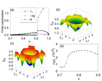
Figure 3: (Color online) Gap and superfluid density for the $f$-wave state at $U/t_{\parallel}=2.2$ and $0.7<n<1.0$. A) The pairing amplitude $\Delta_{A}=-\Delta_{B}=\Delta$ until $n\approx 0.9$. For $n>0.9$, the CDW order starts to coexist with the $f$-wave pairing superfluid, resulting in $f$-wave supersolid state.; B) and C) the lowest energy branch of Bogoliubov excitations at $n=0.89$ and $n=0.78$. For a better visual effect, only the negative eigenvalues are shown. D) The superfluid density $\rho_{s}$ v.s. $n$.

We next study the pairing strength $\Delta_{A}=-\Delta_{B}=\Delta$ in the weak coupling regime with $U/t_{\parallel}=2.2$ in which the validity of the self-consistent mean-field theory is justified. The lattice chiral symmetry ensures that these results are symmetric respect to the filling $n=1$ so that we only present the results for $n\leq 1$. The case of $0<n<0.5$ corresponds to filling in the bottom flat band in which each band eigenstate can be constructed as localized within a single hexagon plaquette presented (see Ref. wu2007 ; wu2008 ). The attractive interaction drives all the plaquette states to touch each other leading to phase separation until the flat band is filled, which will be discussed in a later publication. In Fig. 3 A, we plot $\Delta$ for $0.7<n<1.0$ which corresponds to filling in the dispersive bands. If can be seen that the pairing state remains pure $f$-wave until $n\approx 0.9$. For $n>0.9$, the CDW order parameter $N$ becomes non-zero due to the strong nesting near half-filling, and it contributes to a $s$-wave component to the inter-band pairing, resulting in $\Delta_{A}\neq-\Delta_{B}$ observed in Fig. 3 A. Since the CDW order coexists with the pairing superfluid with dominant $f$-wave component, the phase in the region of $0.9<n<1.0$ is the $f$-wave supersolid state, which is also a novel phase not seen in other systems.

Due to the multi-band structure, this $f$-wave pairing state remains fully gapped for general values of $U/t_{\parallel}$ and $n$. We plot the branch of the lowest energy Bogoliubov excitations for $U/t_{\parallel}=2.2$ and the filling $0.7<n<1$ where the Fermi energy lies in band 2. For $n$ close to 1 in Fig. 3 B ($n=0.89$), the Fermi surfaces form two disconnected pockets around the $\vec{K}$ and $\vec{K}^{\prime}$ away from the nodal lines of $\Delta_{22}(\vec{k})$, thus the spectra are gapped. As $n$ is lowered in Fig. 3 C ($n=0.78$), the Fermi surface becomes connected and intersects with the nodal lines of $\Delta_{22}$. At these intersections, the system in general remains gapped because of the non-zero inter-band pairing $\Delta_{12}(\vec{k})$.

The superfluid density $\rho_{s}$ is plotted in Fig. 3 D for $0.7<n<1.0$ and $U/t_{\parallel}=2.2$, which is defined as

$$\rho_{s}\equiv\frac{\hbar^{2}}{2m^{*}}n_{s}=\lim_{\delta\theta\rightarrow 0}\frac{1}{2}\frac{\partial^{2}E_{MF}}{\partial\delta\theta^{2}}$$ (15)

where $\delta\theta$ is the phase twist across the system boundaries. The behavior of $\rho_{s}$ is very different from that of the pairing gap, which is mostly determined by the states in the dispersive band. $\rho_{s}$ reaches the maximal value of about $0.03t_{\parallel}$ around $n=0.82$ because the filling is close to the van Hove singularity of the density of states, and then drops as we approach the Dirac points at $n=1$. In two dimensional systems, the superfluidity develops below the Kosterlitz-Thouless (K-T) transition temperature $T_{KT}\approx\frac{\pi}{2}\rho_{s}$.

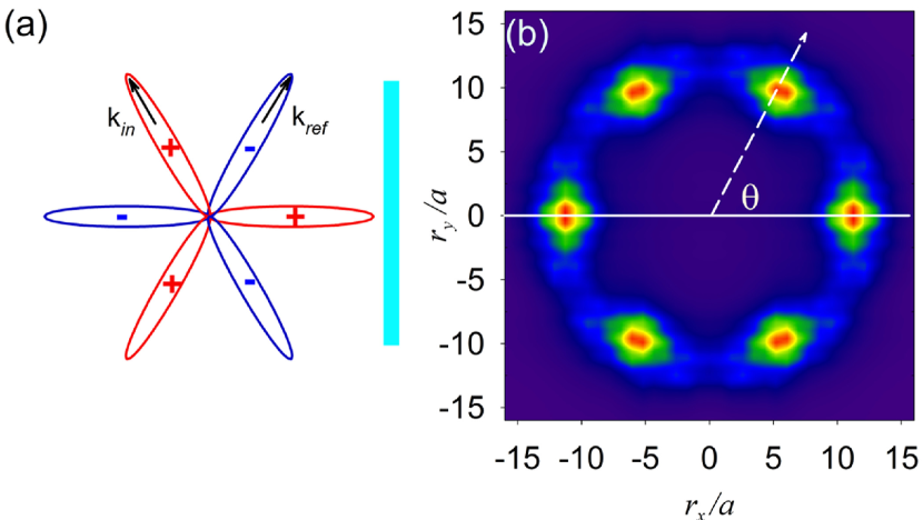
Figure 4: (Color online) (a)The zero energy Andreev bound states appear on the boundary perpendicular to the anti-nodal directions. (b) The zero energy LDOS in real space with the maximal values at $\theta=n\pi/3$ is a signature of the $f$-wave pairing symmetry.

The above mechanism for the $f$-wave pairing works in the weak coupling systems where the non-trivial orbital band structure in momentum space is essential. On the other hand, in the strong coupling limit, i.e., $U$ is much larger than the band width, the Cooper pairing occurs in real space. Two fermions on the same site form a Cooper pair which can tunnel to neighboring sites. As explained in Ref. [hung2009, ], due to the odd parity of the $p$-orbitals, the Josephson coupling amplitude is positive, which favors a phase difference of $\pi$ between two neighbors. Furthermore, its amplitude is much smaller than the CDW coupling because the $\pi$-bonding $t_{\perp}$ is much smaller than $t_{\parallel}$. As a result, the superfluid density is very small in the strong coupling limit although the pairing gap is in the order of $U$.

IV Zero energy Andreev Bound States

One of the most convincing proofs of the unconventional pairing is the existence of the zero energy Andreev bound states at boundaries because of their phase sensitivity hu1994 . Fig. 4 A depicts the situation of the boundary perpendicular to the antinodal lines of the intra-band pairing. The scattering of the Bogoliubov quasi-particles changes momentum from ${\vec{k}}_{in}$ to $\vec{k}_{ref}$ along which the pairing parameters switch the sign as $\Delta_{nn}(\vec{k}_{in})=-\Delta_{nn}(\vec{k}_{ref})$, which gives rise to zero energy Andreev bound states. On the other hand, if the boundary is perpendicular to the nodal lines, no phase changes occur and thus Andreev bound states vanish.

Naturally in the experimental systems with an overall confining trap, the circular edge boundary samples all the orientations. We performed a real space Bogoliubov-de-Gennes calculation degennes as

$$\left(\begin{array}[]{cc}\hat{H}&\hat{\Delta}\\ \hat{\Delta}^{*}&-\hat{H}\\ \end{array}\right)\left(\begin{array}[]{c}u_{n}(i)\\ v_{n}(i)\\ \end{array}\right)=E_{n}\left(\begin{array}[]{c}u_{n}(i)\\ v_{n}(i)\\ \end{array}\right),$$ (22)

where $i$ is the site index in the real space, $H=H_{0}+V_{ex}$, $V_{ex}=\frac{m}{2}\Omega^{2}r_{i}^{2}$ is the harmonic confining potential with parameters $m\Omega^{2}a^{2}=0.001t_{\parallel}$, and $r_{i}$ is the distance from the center of the confining potential to the site $i$. In order to simulate better the realistic experimental situation, we also add the $\pi$-bonding termwu2007a , the hopping with direction perpendicular to the bond direction, into $H_{0}$, and the hopping integral is estimated to be $t_{\perp}/t_{\parallel}=-0.1$. The local density of states (LDOS) at energy $E$ is defined as

$$LD(\vec{r},E) = \frac{1}{N}\sum_{n}|u_{n}(\vec{r})|^{2}\delta(E-E_{n})$$ (23)

$$+ |v_{n}(\vec{r})|^{2}\delta(E+E_{n}),$$

where $N$ is the total number of lattice sites. The numerical result of the zero energy $LD(\vec{r},0)$ is depicted in real space in Fig. 4 B with the parameter values of $U/t_{\parallel}=2.5$ and $\mu=-1.58$ which corresponds to the filling in the center of the trap $n_{c}=0.88$. Fig. 4 B shows that the $LD(\vec{r},0)$ is non-zero only at sites near the boundary, signaling the existence of the zero energy Andreev bound states with six-fold symmetry. The LDOS maxima occur at angles $\theta=n\frac{\pi}{3}~{}(n=1\sim 6)$ which are perpendicular to the antinodal directions shown in Fig. 4 A, and the minima are located at $\theta=(n+\frac{1}{2})\frac{\pi}{3}$. As $U$ increases, the CDW order starts to coexist with the $f$-wave pairing, and it introduces $s$-wave inter-band pairings into the system. Consequently, the scattering process of Bogoliubov quasiparticles described in Fig. 4(a) no longer has a complete sign change in the pairing parameters as discussed above. In this case, we still find the Andreev bound states with six-fold symmetry up to $U/t_{\parallel}=3$, except having finite energy below the excitation gap instead of zero energy.

The zero energy Andreev bound states of this $f$-wave pairing systems have the similar topological origin as those in the superconductors of the $p_{x}+ip_{y}$ symmetry. However, there are important differences. The $f$-wave pairing symmetry presented here is real and anisotropic, which maintains time-reversal symmetry. The edge responses are also anisotropic: the spectra of the zero energy Andreev state are strongest along the boundaries perpendicular to the anti-nodal direction. On the other hand, the $p_{x}+ip_{y}$ pairing symmetry is complex. A spatial rotation operation on the $p_{x}+ip_{y}$ state is equivalent to the change of a global pairing phase, thus its responses to all the boundaries with different directions are all the same. Edge states appear regardless the directions of boundaries. Furthermore, due to its breaking time-reversal symmetry, the edge states in the $p_{x}+ip_{y}$ states carry currents.

V Experimental realization and detection

The experimental realization of this novel $f$-wave state is feasible. To enhance the attractive interaction between spinless fermions, we propose to use atoms with large magnetic moments, such as ¹⁶⁷Er with $m=7\mu_{B}$ on which laser cooling has been performed mcclelland2006 . Compared to another possibility to use the $p$-wave Feshbach resonance, this method has the advantage to maintain the system stability. The interaction between two fermions in $p_{x,y}$-orbitals reads

$$-U = \int d^{3}\vec{r}_{1}d^{3}\vec{r}_{2}V(\vec{r}_{1}-\vec{r}_{2})\Big{\{}[\psi_{p_{x}}(\vec{r}_{1})\psi_{p_{y}}(\vec{r}_{2})]^{2}$$ (24)

$$- \psi^{*}_{p_{x}}(\vec{r}_{1})\psi^{*}_{p_{y}}(\vec{r}_{2})\psi_{p_{x}}(\vec{r}_{2})\psi_{p_{y}}(\vec{r}_{1})\Big{\}},$$

where $\psi_{p_{x},p_{y}}$ are Wannier wavefunctions. The overall dipole interaction can be made attractive by polarizing the magnetic moments parallel to the hexagonal plane, which gives rise to $V(\vec{r}_{1}-\vec{r}_{2})=m^{2}(1-3\cos^{2}\theta)/r^{3}$ where $r=|\vec{r}_{1}-\vec{r}_{2}|$ and $\theta$ is the angle between $\vec{m}$ and $\vec{r}_{1}-\vec{r}_{2}$. We take the laser wavelength $\lambda\approx 600nm$, and then the recoil energy $E_{R}=157nK$. As shown in the Supplementary Information, by choosing $V_{0}/E_{R}=30$, the estimation shows that $U\approx 96nK$ and $t_{\parallel}\approx 0.2E_{R}=31nK$, and thus $U/t_{\parallel}\approx 3$ as chosen above. As shown in Fig. 3 D, the maximal $T_{KT}\approx\frac{\pi}{2}(0.02t_{\parallel})\approx 1\sim 2nK$, which is within the experimentally accessible regime.

A successful detection of the zero energy Andreev bound states will be a convincing proof to the $f$-wave pairing state. The radio-frequency (rf) spectroscopy has been an established tool to determine the pairing gap in cold atom systems chin2004 ; he2005 . It also has a good spatial resolution schirotzek2008 , which makes the direct imaging of the spatial distribution of the zero energy Andreev bound states feasible. The unique symmetry pattern of the zero energy Andreev bound states localized at the trap boundary can be revealed by identifying the locations of the zero energy spectrum determined from the spatially resolved rf spectroscopy. Even for the case in which the Andreev bound states are not at zero energy due to the CDW order, since they are the lowest energy states and below the excitation gap, one can still find that the lowest energy spectra appear near the six locations shown in Fig. 4(b).

VI Conclusion and discussion

In summary, we have proposed the realization of a novel $f$-wave pairing state with spinless fermions which has not been identified in solid state and cold atom systems before. The key reason is the non-trivial $p$-orbital band structure of the honeycomb lattice rather than the strong correlation physics, which renders the above analysis controllable. The $T_{KT}$ is estimated to reach the order of $1nK$ within experimental accessibility. The rf spectroscopy detection of the six-fold symmetry pattern of the zero energy Andreev bound states along the circular boundary will provide a phase sensitive test of the $f$-wave symmetry.

Appendix A Eigenvectors of the band Hamiltonian and the pairing matrix

In this section, we present the spectra of the band Hamiltonian Eq. 1 and the pairing matrix $\Delta_{mn}$. With the four-component spinor operator defined as

$$\hat{\phi}(\vec{k})=(p_{Ax}(\vec{k}),p_{Ay}(\vec{k}),p_{Bx}(\vec{k}),p_{By}(\vec{k}))^{T},$$ (25)

Eq. 1 becomes

$$H_{0} = t_{\parallel}\sum_{k}\hat{\phi}^{\dagger}_{m}(\vec{k})H_{0,mn}(\vec{k})\hat{\phi}_{n}(\vec{k}),$$ (26)

where the matrix kernel $H_{0,mn}(\vec{k})$ takes the structure as

$$\left(\begin{array}[]{cccc}0&0&\frac{3}{4}(e^{i\vec{k}\cdot\vec{e}_{1}}+e^{i\vec{k}\cdot\vec{e}_{2}})&\frac{\sqrt{3}}{4}(e^{i\vec{k}\cdot\vec{e}_{1}}-e^{i\vec{k}\cdot\vec{e}_{2}})\\ 0&0&\frac{\sqrt{3}}{4}(e^{i\vec{k}\cdot\vec{e}_{1}}-e^{i\vec{k}\cdot\vec{e}_{2}})&\frac{1}{4}(e^{i\vec{k}\cdot\vec{e}_{1}}+e^{i\vec{k}\cdot\vec{e}_{2}})+e^{i\vec{k}\cdot\vec{e}_{3}}\\ h.c.&&0&0\\ &&0&0\end{array}\right).$$ (31)

For each momentum $\vec{k}$, $H_{0}(\vec{k})$ is diagonalized as

$$H_{0,lm}(\vec{k})U_{mn}=E_{l}U_{ln}.$$ (32)

The band eigen-operators are expressed as

$$\hat{\psi}_{m}(\vec{k})=\hat{\phi}_{n}(\vec{k})U_{nm}(\vec{k}).$$ (33)

The unitary matrix $U(\vec{k})$ reads

$$U(\vec{k})=\left(\begin{array}[]{c c c c}a^{*}(\vec{k})&e^{-i\frac{\theta_{k}}{2}}b(\vec{k})&e^{-i\frac{\theta_{k}}{2}}b(\vec{k})&a^{*}(\vec{k})\\ -b^{*}(\vec{k})&e^{-i\frac{\theta_{k}}{2}}a(\vec{k})&e^{-i\frac{\theta_{k}}{2}}a(\vec{k})&-b^{*}(\vec{k})\\ a(\vec{k})&e^{i\frac{\theta_{k}}{2}}b^{*}(\vec{k})&-e^{i\frac{\theta_{k}}{2}}b^{*}(\vec{k})&-a(\vec{k})\\ -b(\vec{k})&e^{i\frac{\theta_{k}}{2}}a^{*}(\vec{k})&-e^{i\frac{\theta_{k}}{2}}a^{*}(\vec{k})&b(\vec{k})\end{array}\right),$$ (38)

where

$$a(\vec{k}) = \frac{f_{23}(\vec{k})-f_{31}(\vec{k})}{\sqrt{3N_{0}(\vec{k})}};\ \ \ b(\vec{k})=\frac{f_{12}(\vec{k})}{\sqrt{N_{0}(\vec{k}})};$$

$$\theta_{k} = {\rm arg}\left(\sum_{i}e^{i\vec{k}\cdot\hat{e}_{i}}\right)\in[-\pi,\pi);$$

$$f_{ij}(\vec{k}) = e^{i\vec{k}\cdot\hat{e}_{i}}-e^{i\vec{k}\cdot\hat{e}_{j}};$$

$$N_{0}(\vec{k}) = \frac{8}{3}\Big{[}3-\sum_{1\leq i<j\leq 3}\cos\vec{k}\cdot(\hat{e}_{i}-\hat{e}_{j})\Big{]}.$$ (40)

Using the eigenvector matrix $U(\vec{k})$, the pairing matrix $\Delta_{mn}$ can be spelled out straightforwardly as:

$$\Delta_{mn}(\vec{k}) = \Delta_{A}\left[\hat{U}_{2m}(-\vec{k})\hat{U}_{1n}(\vec{k})-\hat{U}_{1m}(-\vec{k})\hat{U}_{2n}(\vec{k})\right]$$

$$+ \Delta_{B}\left[\hat{U}_{4m}(-\vec{k})\hat{U}_{3n}(\vec{k})-\hat{U}_{3m}(-\vec{k})\hat{U}_{4n}(\vec{k})\right].$$

For the solution of $\Delta_{A}=-\Delta_{B}=\Delta$, we have the pairing matrix as

$$\Delta(\vec{k})=\left(\begin{array}[]{c c c c}\Delta_{1}(\vec{k})&\Delta_{2}(\vec{k})&\Delta_{3}(\vec{k})&0\\ \Delta_{2}(\vec{k})&-\Delta_{1}(\vec{k})&0&-\Delta_{3}(\vec{k})\\ -\Delta_{3}(\vec{k})&0&-\Delta_{1}(\vec{k})&\Delta_{2}(\vec{k})\\ 0&\Delta_{3}(\vec{k})&\Delta_{2}(\vec{k})&\Delta_{1}(\vec{k})\\ \end{array}\right),$$ (46)

where the matrix elements read

$$\Delta_{1}(\vec{k}) = i\frac{16\Delta}{\sqrt{3}N_{0}(\vec{k})}\sin\frac{\sqrt{3}}{2}k_{x}\left[\cos\frac{\sqrt{3}}{2}k_{x}-\cos\frac{3}{2}k_{y}\right],$$

$$\Delta_{2}(\vec{k}) = i\frac{16\Delta}{3N_{0}(\vec{k})}\left[K_{1}(\vec{k})\sin\frac{\theta_{k}}{2}+K_{2}(\vec{k})\cos\frac{\theta_{k}}{2}\right],$$

$$\Delta_{3}(\vec{k}) = \frac{16\Delta}{3N_{0}(\vec{k})}\left[K_{1}(\vec{k})\cos\frac{\theta_{k}}{2}-K_{2}(\vec{k})\sin\frac{\theta_{k}}{2}\right],$$

and

$$K_{1}(\vec{k}) = 4\cos^{4}\frac{k_{y}}{2}+(4\cos^{2}\frac{\sqrt{3}}{2}k_{x}-7)\cos^{2}\frac{k_{y}}{2}$$

$$- \cos\frac{k_{y}}{2}\cos\frac{\sqrt{3}}{2}k_{x}+2\sin^{2}\frac{\sqrt{3}}{2}k_{x},$$

$$K_{2}(\vec{k}) = \sin\frac{k_{y}}{2}(\cos\frac{\sqrt{3}}{2}k_{x}-\cos\frac{k_{y}}{2})$$ (48)

$$\times [(2\cos\frac{k_{y}}{2}+\cos\frac{\sqrt{3}}{2}k_{x})^{2}+\sin^{2}\frac{\sqrt{3}}{2}k_{x}].\ \ \$$

Both the band Hamiltonian Eq. 1 and the interaction Eq. 6 are invariant under the rotation $R_{\frac{\pi}{3}}$. Applying $R_{\frac{\pi}{3}}$ to the band Hamiltonian matrix in momentum space $H_{0}(\vec{k})$, it transforms as

$$H_{0}[\vec{k}^{\prime}=R_{\frac{\pi}{3}}(\vec{k})]=R_{\frac{\pi}{3}}H_{0}(\vec{k})R^{-1}_{\frac{\pi}{3}}$$ (49)

where $R_{\frac{\pi}{3}}$ is defined as

$$R_{\frac{\pi}{3}}=\left(\begin{array}[]{cc}0&r_{\frac{\pi}{3}}\\ r_{\frac{\pi}{3}}&0\\ \end{array}\right),$$ (50)

and

$$r_{\frac{\pi}{3}}=\left(\begin{array}[]{cc}\cos\frac{\pi}{3}&-\sin\frac{\pi}{3}\\ \sin\frac{\pi}{3}&\cos\frac{\pi}{3}\\ \end{array}\right).$$ (51)

Correspondingly, it can be shown directly that

$$R_{\frac{\pi}{3}}\hat{\psi}_{m}(\vec{k})=\,\mathrm{sgn}(m)\hat{\psi}_{m}(\vec{k}^{\prime})$$ (52)

with $\,\mathrm{sgn}(m)=-1$ for $m=1,2$ and $+1$ for $m=3,4$, and $R_{\frac{\pi}{3}}\Delta_{mn}(\vec{k})R_{\frac{\pi}{3}}^{-1}=\,\mathrm{sgn}(n)\,\mathrm{sgn}(m)\Delta_{mn}(\vec{k}^{\prime})$.

Appendix B Calculation of the on-site Hubbard interaction with magnetic dipolar interaction

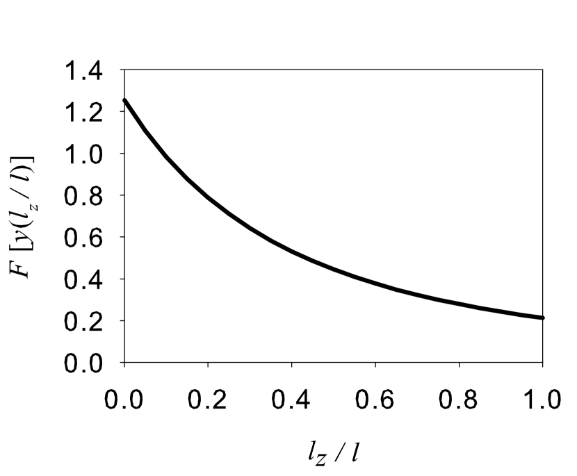
Figure 5: $F[y(l_{z}/l)]$ as a function of $l_{z}/l$.

The optical potential around the center of each optical site can be approximated as

$$V(\vec{r})=\frac{m}{2}\omega^{2}(r_{x}^{2}+r_{y}^{2})+\frac{m}{2}\omega_{z}^{2}r_{z}^{2},$$ (53)

where we assume that the confinement in the $z$-axis is stronger so that $\omega_{z}>\omega$. The wavefunctions for the $p_{x}$ and $p_{y}$ orbitals in this harmonic potential are

$$\psi_{p_{x}}(\vec{r})=C^{\frac{1}{2}}r_{x}\exp\big{\{}-\frac{r_{x}^{2}+r_{y}^{2}}{2l^{2}}-\frac{r_{z}^{2}}{2l_{z}^{2}}\big{\}},$$

$$\psi_{p_{y}}(\vec{r})=C^{\frac{1}{2}}r_{y}\exp\big{\{}-\frac{r_{x}^{2}+r_{y}^{2}}{2l^{2}}-\frac{r_{z}^{2}}{2l_{z}^{2}}\big{\}},$$ (54)

where $C=2l^{-4}l^{-1}_{z}\pi^{-3/2},l=\sqrt{\hbar/m\omega}$, $l_{z}=\sqrt{\hbar/m\omega_{z}}$, and $l_{z}<l$.

With these wavefunctions, the on-site interaction can be evaluated with the direct and exchange terms:

$$-U = \int d^{3}\vec{r}_{1}d^{3}\vec{r}_{2}V(\vec{r}_{1}-\vec{r}_{2})\Big{\{}[\psi_{p_{x}}(\vec{r}_{1})\psi_{p_{y}}(\vec{r}_{2})]^{2}$$ (55)

$$-\psi^{*}_{p_{x}}(\vec{r}_{1})\psi^{*}_{p_{y}}(\vec{r}_{2})\psi_{p_{x}}(\vec{r}_{2})\psi_{p_{y}}(\vec{r}_{1})\Big{\}}$$

$$= C^{2}\int d^{3}\vec{r}d^{3}\vec{R}~{}V(\vec{r})\left(\frac{R_{x}^{2}\,r_{y}^{2}+R_{y}^{2}\,r_{x}^{2}}{2}\right)$$

$$\times F_{1}(\vec{r})F_{2}(\vec{R}),$$

where we have introduced the relative coordinate $\vec{r}=\vec{r}_{1}-\vec{r}_{2}$ and the center of mass coordinate $\vec{R}=(\vec{r}_{1}+\vec{r}_{2})/2$, and defined

$$F_{1}(\vec{r}) = \exp\big{\{}-\frac{r_{x}^{2}+r_{y}^{2}}{2l^{2}}-\frac{r_{z}^{2}}{2l_{z}^{2}}\big{\}},$$

$$F_{2}(\vec{R}) = \exp\big{\{}-\frac{2(R_{x}^{2}+R_{y}^{2})}{l^{2}}-\frac{2R_{z}^{2}}{l_{z}^{2}}\big{\}}.$$ (56)

We propose to use fermionic atoms with large magnetic dipole moments $\vec{m}$. By polarizing the magnetic moments with an external magnetic field, the anisotropic interaction reads

$$V(\vec{r})=\frac{\mu_{0}}{4\pi}\frac{m^{2}[1-3(\hat{m}\cdot\hat{r})]^{2}}{r^{3}}$$ (57)

where $\hat{m}=\vec{m}/m$ and $\hat{r}=\vec{r}/r$, respectively. We assume the polarization angle between $\vec{m}$ and the $xy$-plane is $\theta$, and perform the Gaussian integrals in Eq. 55. The result is expressed analytically as

$$-U = \frac{\mu_{0}}{4\pi}\frac{m^{2}}{2l^{3}}(1-\frac{3}{2}\cos^{2}\theta)F(y),$$ (58)

where

$$F(y) = \sqrt{\frac{2}{\pi}}(1+y)^{3/2}[(3y+1)\tan^{-1}(\frac{1}{\sqrt{y}})$$ (59)

$$- 3\sqrt{y}],$$

and $y$ is a function of $l_{z}/l$ as $y(l_{z}/l)=l_{z}^{2}/(l^{2}-l_{z}^{2})$. $F[y(l_{z}/l)]$ is a monotonic decreasing function of $l_{z}$ as shown in Fig. 5, which reflects that the wavefunctions with a larger $l_{z}$ have smaller overlaps with each other.

The largest attractive interaction can be achieved by polarizing the magnetic moments in the $xy$-plane. If we use the fermionic atom of ¹⁶⁷Er with $m=7\mu_{B}$ and the laser beam with the wavelength $\lambda\approx 600nm$ to construct the honeycomb optical lattice, the recoil energy $E_{R}=h^{2}/2m\lambda^{2}=157nK$ and $l\approx 93(\frac{E_{R}}{V_{0}})^{1/4}$nm. Compared to the realistic band structure calculation with $V_{0}/E_{R}=30$ in Ref. wu2008 , $t_{\parallel}$ is fitted as $t_{\parallel}\approx 0.2E_{R}=31$nK and $l\approx 40$nm. With the choice of $l_{z}/l=0.2$, $U$ reaches reach $96$nK, thus $U/t_{\parallel}\approx 3$ employed in this paper is achieved. Recently, a large number of the fermionic atoms ¹⁶³Dy with $m=10\mu_{B}$ has been successfully cooled and trappedlu2010 . For this atom, the recoil energy $E_{R}=h^{2}/2m\lambda^{2}=161nK$, and $U/t_{\parallel}\approx 3$ can be achieved with the choice of $l_{z}/l=0.55$.

References

- (1) M. Sigrist and K. Ueda, Rev. Mod. Phys. 63, 239 (1991).
- (2) A. J. Leggett, Rev. Mod. Phys. 47, 331 (1975).
- (3) D. D. Osheroff, Rev. Mod. Phys. 69, 667 (1997).
- (4) K. Nelson, Z. Mao, Y. Maeno, and Y. Liu, Science 306, 1151 (2004).
- (5) F. Kidwingira, J. Strand, D. J. V. Harlingen, and Y. Maeno, Science 314, 1267 (2006).
- (6) D. J. Van Harlingen, Rev. Mod. Phys. 67, 515 (1995).
- (7) C. C. Tsuei and J. R. Kirtley, Rev. Mod. Phys. 72, 969 (2000).
- (8) C.-R. Hu, Phys. Rev. Lett. 72, 1526 (1994).
- (9) G. Deutscher, Rev. Mod. Phys. 77, 109 (2005).
- (10) R. Joynt and L. Taillefer, Rev. Mod. Phys. 74, 235 (2002).
- (11) D. E. MacLaughlin, C. Tien, W. G. Clark, M. D. Lan, Z. Fisk, J. L. Smith, and H. R. Ott, Phys. Rev. Lett. 53, 1833 (1984).
- (12) K. Izawa, H. Yamaguchi, Y. Matsuda, H. Shishido, R. Settai, and Y. Onuki, Phys. Rev. Lett. 87, 057002 (2001).
- (13) J. D. Strand, D. J. Van Harlingen, J. B. Kycia, and W. P. Halperin, Phys. Rev. Lett. 103, 197002 (2009).
- (14) F. Dalfovo, S. Giorgini, L. P. Pitaevskii, and S. tringari, Rev. Mod. Phys. 71, 463 (1999).
- (15) A. J. Leggett, Rev. Mod. Phys. 73, 307 (2001).
- (16) I. Bloch, J. Dalibard, and W. Zwerger, Reviews of Modern Physics 80, 885 (2008).
- (17) S. Giorgini, L. P. Pitaevskii, and S. Stringari, Reviews of Modern Physics 80, 1215 (2008).
- (18) C. Chin, R. Grimm, P. Julienne, and E. Tiesinga, Feshbach Resonances in Ultracold Gases, arXiv.org:0812.1496, 2008.
- (19) C. Chin, M. B. A. Altmeyer, S. Riedl, S. Jochim, J. H. Denschlag, and R. Grimm, Science 305, 1128 (2004).
- (20) C. A. Regal, M. Greiner, and D. S. Jin, Phys. Rev. Lett. 92, 40403 (2004).
- (21) M. W. Zwierlein, C. A. Stan, C. H. Schunck, S. M. F. Raupach, A. J. Kerman, and W. Ketterle, Phys. Rev. Lett. 92, 120403 (2004).
- (22) G. B. Partridge, K. E. Strecker, R. I. Kamar, M. W. Jack, and R. G. Hulet, Physical Review Letters 95, 020404 (2005).
- (23) T.-L. Ho and R. B. Diener, Phys. Rev. Lett. 94, 090402 (2005).
- (24) V. Gurarie and L. Radzihovsky, Annals of Physics 322, 2 (2007).
- (25) C.-H. Cheng and S.-K. Yip, Phys. Rev. Lett. 95, 070404 (2005).
- (26) J. Zhang, E. G. M. van Kempen, T. Bourdel, L. Khaykovich, J. Cubizolles, F. Chevy, M. Teichmann, L. Tarruell, S. J. J. M. F. Kokkelmans, and C. Salomon, Phys. Rev. A 70, 30702(R) (2004).
- (27) J. P. Gaebler, J. T. Stewart, J. L. Bohn, and D. S. Jin, Physical Review Letters 98, 200403 (2007).
- (28) J. Fuchs, C. Ticknor, P. Dyke, G. Veeravalli, E. Kuhnle, W. Rowlands, P. Hannaford, and C. J. Vale, Physical Review A (Atomic, Molecular, and Optical Physics) 77, 053616 (2008).
- (29) Y. Inada, M. Horikoshi, S. Nakajima, M. Kuwata-Gonokami, M. Ueda, and T. Mukaiyama, Physical Review Letters 101, 100401 (2008).
- (30) G. Grynberg, B. Lounis, P. Verkerk, J. Courtois, and C. Salomon, Phys. Rev. Lett. 70, 2249 (1993).
- (31) C. Wu, D. Bergman, L. Balents, and S. Das Sarma, Phys. Rev. Lett. 99, 70401 (2007).
- (32) C. Wu and S. Das Sarma, Phys. Rev. B 77, 235107 (2008).
- (33) S. Z. Zhang, H. H. Hung, and C. Wu, Proposed realization of itinerant ferromagnetism in optical lattices, arXiv.org:0805.3031, 2008.
- (34) C. Wu, Phys. Rev. Lett. 100, 200406 (2008).
- (35) C. Wu, Phys. Rev. Lett. 101, 186807 (2008).
- (36) P. G. De Gennes, Superconductivity of Metals and Alloys (Addison-Wesley Publishing Company, ADDRESS, 1989).
- (37) J. J. McClelland and J. L. Hanssen, Physical Review Letters 96, 143005 (2006).
- (38) Y. He, Q. Chen, and K. Levin, Phys. Rev. A 72, 011602 (2005).
- (39) A. Schirotzek, Y. il Shin, C. H. Schunck, and W. Ketterle, Phys. Rev. Lett. 101, 140403 (2008).
- (40) M. Lu, S. H. Youn, and B. L. Lev, Phys. Rev. Lett. 104, 063001 (2010).
- (41) H. h. Hung, W. C. Lee, C. Wu, arxiv:0910.0507.