Observational Limits on Type 1 AGN Accretion Rate in COSMOS

Abstract

We present black hole masses and accretion rates for 182 Type 1 AGN in COSMOS. We estimate masses using the scaling relations for the broad H$\beta$, Mgii, and Civ emission lines in the redshift ranges $0.16<z<0.88$, $1<z<2.4$, and $2.7<z<4.9$. We estimate the accretion rate using an Eddington ratio $L_{I}/L_{Edd}$ estimated from optical and X-ray data. We find that very few Type 1 AGN accrete below $L_{I}/L_{Edd}\sim 0.01$, despite simulations of synthetic spectra which show that the survey is sensitive to such Type 1 AGN. At lower accretion rates the BLR may become obscured, diluted or nonexistent. We find evidence that Type 1 AGN at higher accretion rates have higher optical luminosities, as more of their emission comes from the cool (optical) accretion disk with respect to shorter wavelengths. We measure a larger range in accretion rate than previous works, suggesting that COSMOS is more efficient at finding low accretion rate Type 1 AGN. However the measured range in accretion rate is still comparable to the intrinsic scatter from the scaling relations, suggesting that Type 1 AGN accrete at a narrow range of Eddington ratio, with $L_{I}/L_{Edd}\sim 0.1$.

1. Introduction

Supermassive black holes (SMBHs) reside in almost all local galaxies (Kormendy & Richstone, 1995; Richstone et al., 1998). The mass of the SMBH is observed to be tightly correlated with the mass, luminosity, and velocity dispersion of the host galaxy bulge (e.g., Magorrian et al., 1998; Gebhardt et al., 2000; Ferrarese & Merritt, 2000). SMBHs grow by accretion as active galactic nuclei (AGN), and all massive galaxies have one or more of these active phases (Soltan, 1982; Magorrian et al., 1998; Marconi et al., 2004). More luminous AGN are observed to peak at higher redshift (Ueda et al., 2003; Brandt & Hasinger, 2005; Bongiorno et al., 2007), exhibiting “downsizing” by analogy to the preference of luminous and massive galaxies to form at high redshifts. Both downsizing and the correlations between SMBH and the host bulge suggest that the growth of AGN and the formation of galaxies are directly connected through feedback (Silk & Rees, 1998; Di Matteo, Springel, & Hernquist, 2005).

Understanding the role of AGN in galaxy evolution requires measurements of SMBH mass and accretion over the cosmic time. The SMBH mass can be directly estimated by modeling the dynamics of nearby gas or stars, but this requires high spatial resolution and is limited to HST observations of nearby galaxies. Reverberation mapping of Type 1 AGN (with broad emission lines) uses the time lag between variability in the continuum and the broad line region (BLR) to estimate the radius of the broad line region, $R_{BLR}=ct_{lag}$ (for a review, see Peterson & Bentz, 2006). Then, if the broad line region virially orbits the source of the continuum emission, the SMBH mass is $M_{BH}=fR_{BLR}v_{fwhm}^{2}$, where $f$ represents the unknown BLR geometry and $v_{fwhm}$ is the velocity width of the broad emission line. This technique has many potential systematic errors (Krolik, 2001; Marconi et al., 2008), but its mass estimates agree with those from dynamical estimators (Davies et al., 2006; Onken et al., 2007) and those from the $M_{BH}$-$\sigma*$ correlation (Onken et al., 2004; Greene & Ho, 2006). In principle, reverberation mapping can be applied to AGN at any redshift, but in practice, the need for many periodic observations has limited reverberation mapping mass estimates to only $\sim$35 local AGN.

Instead, the vast majority of AGN mass estimates have come from a set of scaling relations. Reverberation mapping data led to the discovery that $R_{BLR}$ correlates with the continuum luminosity (Kaspi et al., 2000), with $R_{BLR}\sim L^{\alpha}$, where $\alpha\sim 0.5$ (Bentz et al., 2006; Kaspi et al., 2007). This allows for estimates of $M_{BH}$ from single epoch spectra with scaling relations:

$$\log\left(\frac{M_{BH}}{M_{\odot}}\right)=A+B\log(\lambda L_{\lambda})+2\log(v_{FWHM})$$ (1)

Some authors replace the continuum luminosity with the recombination line luminosity (Wu et al., 2004) or the FWHM with the second moment $\sigma$ (Collin et al., 2006), yielding minor systematic differences in estimated $M_{BH}$ (Shen et al., 2008). While these scaling relations are based upon reverberation mapping of only local AGN, the method is based upon the ability of the central engine to ionize the broad line region (Kaspi et al., 2000), and there is no physical reason to suggest that the ionization of AGN should evolve with redshift (Dietrich & Hamann, 2004; Vestergaard, 2004). Thus the scaling relations can be used to study the distribution and evolution of Type 1 AGN masses. Kollmeier et al. (2006) showed that Type 1 AGN tend to accrete at a narrow range of Eddington ratio, typically $0.01L_{Edd}<L<L_{Edd}$. Kollmeier et al. (2006) suggest a minimum accretion rate for Type 1 AGN, with AGN of lower accretion rate observed as “naked” Type 2 AGN without a broad line region (Hopkins et al., 2008). Gavignaud et al. (2008) additionally suggest that lower luminosity Type 1 AGN accrete less efficiently than brighter quasars.

In this work we report black hole masses and study the demographics of 182 Type 1 AGN in the Cosmic Evolution Survey (COSMOS, Scoville et al., 2007). We introduce the data and outline our spectral fitting in §2, and discuss the black hole masses, their associated errors, and our completeness in §3. We close with discussion of Type 1 AGN accretion rates in §4. All luminosities are calculated using $h=0.70$, $\Omega_{M}=0.3$, $\Omega_{\Lambda}=0.7$.

2. Observational Data

2.1. Sample

The Cosmic Evolution Survey (COSMOS, Scoville et al., 2007) is a 2 deg² HST/ACS survey (Koekemoer et al., 2007) with ancillary deep multiwavelength observations. The depth of COSMOS over such a large area is particularly suited to the study of low-density, rare targets like active galactic nuclei (AGN). The most efficient way to select AGN is by their X-ray emission, and XMM-Newton observations of COSMOS (Cappelluti et al., 2008) reach fluxes of $1\times 10^{-15}$ cgs and $6\times 10^{-15}$ cgs in the 0.5-2 keV and 2-10 keV bands, respectively. The matching of X-ray point sources to optical counterparts is described by Brusa et al. (2007) and Brusa et al. (2009). Trump et al. (2009) performed a spectroscopic survey of XMM-selected AGN in COSMOS, revealing 288 Type 1 AGN with X-ray emission and broad emission lines in their spectra. Here we investigate a chief physical property, the black hole mass, for the Type 1 AGN in this survey.

From the Trump et al. (2009) sample, we choose the 182 Type 1 AGN with high-confidence redshifts and with H$\beta$, Mgii, or Civ present in the observed wavelength range. That is, we select only $z_{\rm conf}\geq 3$ AGN, empirically determined by Trump et al. (2009) to be at least 90% likely to have the correct classification and redshift. All of the Type 1 AGN spectra are dominated by blue power-law continua, with no obvious (beyond the noise) absorption line signature from the host galaxy. The broad emission line requirement restricts us to the redshift ranges $0.16<z<0.88$, $1<z<2.4$, and $2.7<z<4.9$. At these redshifts the AGN spectroscopy is $>90\%$ complete to $i_{\rm AB}^{+}<22$ (see Figure 13 of Trump et al., 2009), where $i_{\rm AB}^{+}$ is the AB magnitude from the COSMOS CFHT observations. Our ability to measure a broad line width, however, is a slightly more complicated function of the spectral signal to noise. We characterize our completeness as a function of broad line width and S/N in §3.2.

The majority (133) of the 182 AGN have spectra from Magellan/IMACS (Bigelow et al., 1998), with wavelength coverage from 5600-9200Å and $\sim$10$\AA$ resolution. The remaining bright 49 quasars have publicly available spectra from the Sloan Digital Sky Survey (SDSS) quasar catalog (Schneider et al., 2007), with 3800-9200Å wavelength coverage and $\sim$3Å resolution. The resolution of both surveys is more than sufficient for measuring broad emission line widths; our narrowest broad emission line is 1300 km/s wide, compared to the resolution limits of IMACS ($\sim$600 km/s) and the SDSS ($\sim$200 km/s).

2.2. Spectral Fitting

The optical/UV spectrum of a Type 1 AGN can be roughly characterized as a power-law continuum, $f_{\nu}\propto\nu^{-\alpha}$, with additional widespread broad iron emission and broad emission lines (Vanden Berk et al., 2001). We followed Kelly et al. (2008) to model the spectra, using an optical Fe template from Veron-Cetty, Joly, & Veron (2004) and a UV Fe template from Vestergaard & Wilkes (2001). Each spectrum was simultaneously fit with a power-law continuum and an iron template using the Levenberg-Marquardt method for nonlinear $\chi^{2}$ minimization. We calculated the continuum luminosity from the power-law fit parameters. Light from the host galaxy can artificially inflate the estimated AGN continuum luminosity, as shown by Bentz et al. (2006) for the 35 AGN with reverberation mapping data. In particular, Bentz et al. (2006) find that at 5100Å, host galaxies contribute $\sim$20% of the measured flux for AGN with ${\lambda}L_{5100}>10^{44}$ erg/s, and $\sim$45% of the flux for AGN of ${\lambda}L_{5100}<10^{44}$ erg/s. We note that the expected host contamination at $L_{3000}$ or $L_{1350}$ is much smaller, since most host galaxies (excepting very active star-forming hosts) have much less flux blueward of the 4000Å break. So for the majority of our sample, the 150 AGN with masses measured from Mgii or Civ, we do not expect host contamination to be significant. However, the 15 AGN with ${\lambda}L_{3000}<10^{44}$ erg/s and H$\beta$-derived masses may have luminosity estimates overestimated by a factor of two, leading to black hole masses and Eddington ratios systematically overestimated by $\sim$0.15 dex. Future work in COSMOS will use host decompositions from HST/ACS images of $z<1$ AGN to better characterize host contamination, but in this work we make no corrections for host galaxy flux.

To fit the broad emission lines we subtracted the continuum and Fe emission fits. Narrow absorption lines and narrow emission lines near the broad line (e.g., [Oiii]$\lambda$4959 and [Oiii]$\lambda$5007 near H$\beta$) were fit by the sum of 1-2 Gaussian functions and removed. Again following Kelly et al. (2008), each remaining broad emission line profile was fit by the sum of 1-3 Gaussian functions, minimizing the Bayesian information criterion (BIC, Schwartz, 1979). Roughly, 2 Gaussians provided the best fit for $\sim$40% of line profiles, while 1 or 3 Gaussians each provided the best fit for $\sim$30% of line profiles. All fitting was interactive and inspected visually, and if the multiple-Gaussian fit revealed a narrow ($<600$ km/s) line in an H$\beta$ emission line, the component was attributed to non-BLR origins and was removed. The FWHM was calculated directly from the multiple-Gaussian fit in order to minimize the effects of noise in the original spectra. The multiple-Gaussian fit was robust to a variety of line profiles, and simulated spectra (see §3.2) revealed measured FWHM errors of only $\sigma_{FWHM}/FWHM\sim 10\%$.

Three examples of spectra with fitted continua and continuum-subtracted line profiles are shown in Figure 1. The spectra are representative of typical fits for each of the Civ, Mgii, and H$\beta$ emission lines. At left the power-law and iron emission fits are shown by the dashed blue lines. The right panel shows the multiple-Gaussian line profile fits as dashed blue lines, with the continuum-subtracted line profile shifted above by an arbitrary amount for clarity. The fit to the H$\beta$ line profile in the bottom right panel includes a narrow ($\sigma=433$ km/s) Gaussian which is not associated with the BLR and was removed. Even for noisy spectra like the middle panel, the spectral fitting provides a robust continuum and isolates the emission line.

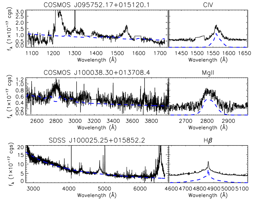
Figure 1.— Three spectra, representing fits and line profiles for Type 1 AGN with Civ (top), Mgii (middle), and H$\beta$ (bottom). In the left panels, the spectra are shown by black histograms, and the dashed blue lines are the power-law plus iron emission continuum fits. At right, the blue dashed line shows the multiple-Gaussian fit to the continuum-subtracted line profiles, which are shown in black and shifted above for clarity. The fit to the H$\beta$ line profile in the lower right panel includes a narrow ($\sigma=433$ km/s) Gaussian which was removed before calculating the broad emission line width. The top two spectra were observed with Magellan/IMACS and have $\sim$10$\AA$ resolution, while the bottom spectrum comes from the SDSS and has $\sim$3$\AA$ resolution.

3. Estimated Black Hole Masses

We estimate black hole masses using our measured broad line velocity widths and the scaling relations of Vestergaard et al. (in prep.) for Mgii and Vestergaard & Peterson (2006) for H$\beta$ and Civ. These relations all take the form of Equation 1, with ${\lambda}L_{\lambda}$ in units of $10^{44}$ erg/s and $v_{FWHM}$ in units of 1000 km/s; $A=6.91$, $B=0.50$, and $\lambda=5100$Å for H$\beta$; $A=6.86$, $B=0.50$, and $\lambda=3000$Å for Mgii; $A=6.66$, $B=0.53$, and $\lambda=1350$Å for Civ. The Mgii relation was derived from SDSS quasars with both Civ and Mgii in the spectrum, and it is designed to produce black hole masses consistent with those measured from Civ. In our sample, we measure H$\beta$ for 32 AGN, Mgii for 134 AGN, and Civ for 38 AGN (19 SDSS AGN have both Mgii and Civ, and 3 have both H$\beta$ and Mgii). AGN with estimates of $M_{BH}$ from two different emission lines are treated as two separate objects in our subsequent analyses.

Table 1 presents the catalog of black hole masses and line measurements. AGN with both Mgii and Civ or both H$\beta$ and Mgii present have two entries in Table 1, one for each emission line. The full catalog then contains 204 entries: 182 Type 1 AGN with $M_{BH}$ estimates, 22 of which have two sets of broad emission line measurements. The black hole masses are shown with continuum luminosity (calculated from the power-law fit) and redshift in Figure 2. The diagonal tracks in the figure represent Eddington ratios using a bolometric correction of 5 for ${\lambda}L_{3000}$ (Richards et al., 2006). We also show a comparison sample of brighter SDSS quasars (Kelly et al., 2008) in order to highlight the lower black hole masses probed by COSMOS.

Table 1COSMOS Type 1 AGN Black Hole Mass Catalog

Object	Redshift	S/N	$\log({\lambda}L_{3000\AA})$	$\log(L_{0.5-2\rm keV})$	Line	FWHM	$\log(M_{BH})$
(J2000)		(per pixel)	[erg/s]	[erg/s]		(km/s)	$[M_{\odot}]$
SDSS J095728.34+022542.2	1.54	7.0	45.00	44.47	MgII	4491	8.665
SDSS J095728.34+022542.2	1.54	7.0	45.00	44.47	CIV	2776	8.135
COSMOS J095740.78+020207.9	1.48	17.9	43.46	44.41	MgII	6701	8.244
SDSS J095743.33+024823.8	1.36	3.4	44.60	43.50	MgII	3472	8.243
COSMOS J095752.17+015120.1	4.17	7.3	45.19	44.36	CIV	4603	8.656
COSMOS J095753.49+024736.1	3.61	4.8	44.14	44.53	CIV	2629	7.997
SDSS J095754.11+025508.4	1.57	6.1	45.07	44.45	MgII	4500	8.701
SDSS J095754.70+023832.9	1.60	8.0	45.17	43.69	MgII	3361	8.498
SDSS J095754.70+023832.9	1.60	8.0	45.17	43.69	CIV	6384	8.946
SDSS J095755.08+024806.6	1.11	8.7	44.92	44.08	MgII	3574	8.426
COSMOS J095755.34+022510.9	2.74	3.2	44.38	-1.00	CIV	3879	8.074
COSMOS J095755.48+022401.1	3.10	19.9	45.28	45.00	CIV	3527	8.436

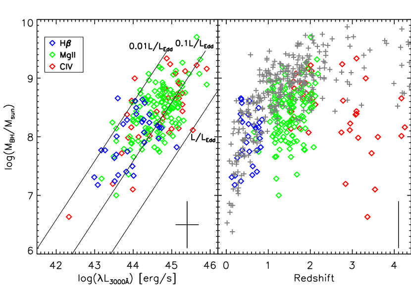
Figure 2.— Black hole mass versus optical luminosity and redshift for 182 Type 1 AGN in COSMOS. The black hole masses are derived from the broad line velocity widths of H$\beta$ (blue diamonds), Mgii (green diamonds), and Civ (red diamonds) depending on the redshift (Vestergaard & Peterson, 2006; Vestergaard et al., in prep.). The black hole masses have uncertainties of $\sim$0.4 dex from the scaling relations (Krolik, 2001; Shen et al., 2008), as shown by the typical error bars are shown in the lower right of each panel (the redshift error is $\lesssim 1\%$). The diagonal tracks at left represent Eddington ratios, assuming a bolometric correction of $L_{bol}=5({\lambda}L_{3000})$ (Richards et al., 2006). At right the gray crosses show scaling relation masses of SDSS quasars (Kelly et al., 2008). The depth of COSMOS allows us to probe low mass and weakly accreting SMBHs, revealing that $L/L_{Edd}\lesssim 0.01$ Type 1 AGN do not exist.

3.1. Error

The scaling relations have uncertainties of $\sim$0.4 dex, although there may be larger systematic uncertainties (Krolik, 2001; Collin et al., 2006; Fine et al., 2008; Marconi et al., 2008). Measurement errors in the luminosity and emission line FWHM also contribute, but the uncertainty from the scaling relations dominates. We test the luminosity error in the left panel of Figure 3, which compares the luminosity estimates from this work to duplicate estimates from Merloni et al. (in prep.). The luminosity estimates of Merloni et al. (in prep.) use independent redshifts from VLT/VIMOS spectra and are calculated from a fit to the IR to X-ray multiwavelength spectral energy distribution, instead of from the optical spectrum itself (as in this work). The scatter between the two luminosity estimates is $\sigma=0.25$ dex. The Type 1 AGN in COSMOS have an average variability of $\sim$0.15 dex (Salvato et al., 2009), the remaining luminosity scatter can be attributed to the different methods of estimates. Since $M_{BH}\sim L^{0.5}$, our luminosity error contributes very little to the overall $M_{BH}$ uncertainty.

Line measurements of synthetic spectra (described in §3.2 below) show that our FWHM error is only $\sigma_{FWHM}/FWHM\sim 10\%$ at $i_{\rm AB}^{+}\sim 22$. The right panel of Figure 3 compares the duplicate estimates of $M_{BH}$ for spectra with two broad emission lines. Red diamonds indicate spectra with both Mgii and H$\beta$, while blue crosses indicate both Mgii and Civ. The scatter between the different estimates is only $\sigma=0.36$ dex, nearly the same as the expected intrinsic scatter for $M_{BH}$. This suggests that the statistical error in the mass estimators is not correlated to the choice of emission line (see also Kelly & Bechtold, 2007). If there were systematic offsets in the mass estimators, they would cause a constant shift in the mass estimate for each line, and therefore would not contribute to the scatter between two lines. The statistical intrinsic scatter, however, would not “cancel” in such a way. Because the scatter between lines is comparable to the expected intrinsic scatter, our estimates of $M_{BH}$ probably do not have significant systematic errors.

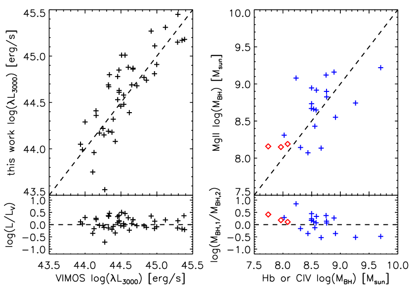
Figure 3.— At left, the luminosity estimates for 48 AGN in this work are compared to estimates of the same objects from Merloni et al. (in prep.), which have independent redshifts from VLT/VIMOS spectra and are calculated from a fit to the multiwavelength SED. The scatter between the two luminosity estimates is $\sigma=0.25$ dex, which contributes very little to the overall scatter in $M_{BH}$. At right, $M_{BH}$ estimates are compared for the 22 spectra with two emission lines (either Mgii and H$\beta$, red diamonds, or Mgii and Civ, blue crosses). The scatter between separate $M_{BH}$ estimates is only $\sigma=0.36$ dex, indicative that the intrinsic scatter of $\sim$0.4 dex dominates the $M_{BH}$ error.

3.2. Completeness

Previous work (Trump et al., 2009) tested the completeness of the Type 1 AGN sample, with simulated spectra showing that Type 1 AGN are correctly identified (with high confidence redshifts) at 90% completeness to S/N$\gtrsim$2.87. But even for correctly identified Type 1 AGN, our measurements of $M_{BH}$ are roughly limited by spectral S/N and FWHM, since we cannot identify or measure broad emission lines for spectra that have lines so broad that they become confused with noise or the Fe emission. To test these limits, we create 100 synthetic spectra of Type 1 AGN with Mgii in the observed wavelength range. We choose Mgii because it is the most common line used for our $M_{BH}$ calculations and also because it is the broad emission line most contaminated by widespread iron emission. These synthetic spectra are formed by making a composite of all $1<z<2.4$ observed spectra, then removing the rest-frame $2700\AA<\lambda<2900\AA$ Mgii region. To each of the 100 spectra we then re-add a Mgii region with random FWHMs and line areas, and then each spectrum has random noise added. We choose the line areas and noise to be normally distributed in the ranges of measured line area and S/N in the original spectra, while the FWHMs are chosen to probe our sensitivity to the broadest line widths, FWHM$\gtrsim 10000$ km/s.

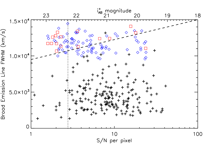
Figure 4.— The broad emission line FWHM and S/N for our 182 Type 1 AGN are shown as black crosses. The upper axis shows the $i_{\rm AB}^{+}$ magnitude scale which roughly corresponds to the S/N (from Figure 11 of Trump et al., 2009). Also shown are the measured FWHM and S/N for 100 simulated Type 1 AGN spectra: blue diamonds represent spectra we can correctly identify and measure, while red squares represent synthetic spectra that we incorrectly identify or cannot properly measure FWHM. The dashed line shows the limit to which we correctly identify and measure $>95\%$ of synthetic spectra. The dotted vertical line shows the 90% completeness to identifying and assigning high-confidence redshifts to Type 1 AGN, from additional simulations (Trump et al., 2009). The lack of high-FWHM AGN identified in COSMOS is not from selection effects, since we can correctly identify and measure synthetic Type 1 AGN with much broader lines at S/N$>3$.

We show the FWHM and S/N of both the observed and simulated spectra in Figure 4. The blue diamonds and red squares represent the simulated spectra that we successfully measure and those we miss, respectively. The vertical dotted line shows the sample’s 90% completeness limit for correctly identifying high-confidence Type 1 AGN. The dashed line shows the limit to where we can measure broad emission lines, corresponding to $>95\%$ completeness since only one “missed” synthetic spectrum lies below the line. The observed Type 1 AGN tail off well before the dashed line. Translating FWHM and magnitude into black hole mass, as an example, a Type 1 AGN with $i_{\rm AB}^{+}\sim 22$ at $z\sim 1.7$ with a Mgii profile of FWHM$=10000$ km/s would have $\log(M_{BH}/M_{\odot})\sim 10.6$ and $L/L_{Edd}\sim 0.0002$. We do not detect such objects in our sample, yet our simulations show that they do not lie beyond our detection limits.

4. Discussion

In Figure 2 all Type 1 AGN lie within the region of $0.01\lesssim L/L_{Edd}\lesssim 1$, a result supported by Kollmeier et al. (2006). This implies that the broad emission line region of Type 1 AGN might become undetectable as the accretion drops below $L\sim 0.01L_{Edd}$. Such objects might be observed as unobscured Type 2 AGN, the possible remnants of “dead” Type 1 AGN whose accretion disk geometries changed as their accretion rates fell (e.g., Hopkins et al., 2008). Or these low accretion rate AGN may be diluted, with their emission falling below the light of their host galaxy. The AGN emission may also be unable to blow out local obscuring material, causing their BLR to lie undetected behind obscuration.

The Eddington ratio (accretion rate) with black hole mass, luminosity, and redshift for our Type 1 AGN. Eddington ratio was calculated using an intrinsic luminosity $L_{I}$ estimated from ${\lambda}L_{3000}$ and $L_{\rm 0.5-2keV}$ using the relations of Marconi et al. (2004). Diamonds represent individual objects with masses estimated from H$\beta$ (blue), Mgii (green), and Civ (red). The large crosses in the top plots show the mean accretion rate in each bin of $M_{BH}$ or redshift, while the gray lines at the bottom show the standard deviation (the square root of the second moment) in each bin. The dispersion deviation is also shown by the vertical error bar in the top plots. Bins were chosen to each have the same number of objects. Selection effects cause the apparent trends of $L_{I}/L_{Edd}$ decreasing with $M_{BH}$ and increasing with redshift, but the increase of $L_{I}/L_{Edd}$ with ${\lambda}L_{3000}$ is a physical effect caused by changes in the accretion disk. The dispersion is generally $\sim$0.4 dex, higher than that of previous, less sensitive surveys.

To study the accretion rates of our AGN, we calculate the intrinsic luminosity from our measured ${\lambda}L_{3000}$ and $L_{\rm 0.5-2keV}$, using the relations of Marconi et al. (2004):

$$\log[L_{I}/({\lambda}L_{3000})]=0.65-0.067\mathcal{L}+0.017\mathcal{L}^{2}-0.0023\mathcal{L}^{3}$$ (2)

$$\log(L_{I}/L_{0.5-2})=1.65+0.22\mathcal{L}+0.012\mathcal{L}^{2}-0.0015\mathcal{L}^{3}$$ (3)

Here $\mathcal{L}=\log(L_{I})-45.58$ and all luminosities are in units of erg/s. The intrinsic luminosity $L_{I}$ is designed to be a bolometric luminosity which excludes reprocessed (IR) emission, so that the Eddington ratio $L_{I}/L_{Edd}$ represents a robust measure of the accretion onto the black hole. We use the Newton method to solve each equation for $L_{I}$ from ${\lambda}L_{3000}$ and $L_{0.5-2}$. We then average the two values of $L_{I}$ for our final value (excepting 7 AGN where we estimate $L_{I}$ from ${\lambda}L_{3000}$ only because they lack soft X-ray detections).

We show the Eddington ratios of our Type 1 AGN with $M_{BH}$, ${\lambda}L_{3000}$, and redshift in Figure 4. The diamonds show individual objects, while the solid lines show the means and scatter in equal-sized bins. The scatter (the standard deviation of the mean) is calculated as the square root of the second moment of the data in each bin. Our mean Eddington ratio for all Type 1 AGN is $L_{I}/L_{Edd}\sim 0.1$, lower than the value of $L_{I}/L_{Edd}\sim 0.3$ found in previous surveys (Kollmeier et al., 2006; Gavignaud et al., 2008). This is partly explained by the depth of COSMOS: Kollmeier et al. (2006) noted that their $R\leq 21.5$ AGES sample was only complete to $L_{I}/L_{Edd}\sim 0.1$, while our simulations in §3.2 show that COSMOS can reach much weaker accretors. In addition, the center panel of Figure 4 shows that accretion rate may increase with optical/UV luminosity, suggesting an additional reason for our lower mean Eddington ratio: most of the Kollmeier et al. (2006) and Gavignaud et al. (2008) AGN have ${\lambda}L_{3000}>10^{45}$ erg/s, where our AGN have $L_{I}/L_{Edd}\sim 0.2$. The majority of our AGN have ${\lambda}L_{3000}<10^{45}$ erg/s and so we find a lower mean accretion rate.

The apparent decrease in accretion rate with black hole mass and the apparent increase in accretion rate with redshift can be explained by selection effects: low accretion rate AGN are more difficult to detect if they are also low mass or at higher redshift. The increase in accretion rate with optical luminosity, however, is also observed by Gavignaud et al. (2008) and is probably a physical effect. We performed a linear regression analysis of the correlation between accretion rate and optical luminosity using the publicly available IDL program linmix_err.pro (Kelly, 2007). Using errors of 0.25 dex in $\log({\lambda}L_{3000})$ and 0.4 dex in $\log(L_{I}/L_{Edd})$, linear regression indicates that $\log(L_{I}/L_{Edd})\sim(0.28\pm 0.06)\log({\lambda}L_{3000})$. In other words, accretion rate is correlated with opticaly luminosity at the 4.8$\sigma$ level. As a Type 1 AGN increases in accretion rate, its optical emission becomes a larger fraction of its total bolometric output because its cool accretion disk emits more brightly. This is consistent with the results of Kelly et al. (2008), which show that $\alpha_{OX}$ (the ratio between optical/UV and X-ray flux) becomes more X-ray quiet with accretion rate. Thus a more rapidly accreting Type 1 AGN has more of its emission in its cool (optical) disk than in its hot (X-ray) corona, possibly because the disk grows larger or thicker as the accretion rate approaches the Eddington limit.

The scatter (square root of the second moment) in $L_{I}/L_{Edd}$, shown in the bottom panels of Figure 4, is typically only $\sim$0.4 dex in each bin. This is greater than previously measured dispersions (Kollmeier et al., 2006; Gavignaud et al., 2008; Fine et al., 2008), and indicates that COSMOS is more sensitive to low accretion rate Type 1 AGN than previous studies. Yet it is remarkable that the dispersion is not larger than the scatter from the scaling relations: the intrinsic dispersion in Eddington ratio might then be $\sim$0, with nearly all Type 1 AGN of a given mass, luminosity, and/or redshift accreting at a very narrow range of of accretion rates. Fine et al. (2008) note that at such low measured dispersions, if the intrinsic dispersion in accretion rate is much greater than 0, then the BLR cannot be in a simple virial orbit. Accurate scaling relations would then require a luminosity-dependent ionization parameter (Marconi et al., 2008) or a more complex BLR geometry (Fine et al., 2008). We note, however, that the myriad uncertainties involved in estimating $L_{I}/L_{Edd}$ make concrete conlusions difficult. And although we find significant evidence that $L_{I}/L_{Edd}<0.01$ Type 1 AGN do not exist (or are very rare), the spectroscopic flux limit may still miss some $L_{I}/L_{Edd}\sim 0.01$ AGN at lower luminosities.

5. Summary

The black hole masses of Type 1 AGN in COSMOS indicate that Type 1 AGN accrete at a narrow range of high efficiencies, $L_{I}/L_{Edd}\sim 0.1$. When the accretion rate of an AGN lowers, less of its luminosity is emitted optically. When a Type 1 AGN accretion rate drops below $L_{I}/L_{Edd}\sim 0.01$ the BLR becomes invisible, due to obscuration, dilution, or an altered accretion disk geometry. We additionally measure higher dispersions in accretion rate than previous, less sensitive surveys, although the dispersion is still no larger than the intrinsic uncertainty in the scaling relations. Kelly et al. (2008) find that the bolometric correction depends on black hole mass, and Vasudevan & Fabian (2009) find that it correlates with Eddington ratio. This makes characterizing the distributions of $L_{I}/L_{Edd}$ and its scatter rather difficult. We partially mitigate the systematic uncertainties by using both ${\lambda}L_{3000}$ and $L_{0.5-2}$ to estimate $L_{I}$. Future work in COSMOS will use more accurate bolometric luminosities calculated from the full multiwavelength dataset.

References

- Bentz et al. (2006) Bentz, M. C., Peterson, B. M., Pogge, R. W., Vestergaard, M., & Onken, 2006, C. A. ApJ, 644, 133
- Bentz et al. (2006) Bentz, M. C., Peterson, B. M., Pogge, R. W., & Vestergaard, M. 2008, ApJ, 694, 166
- Bigelow et al. (1998) Bigelow, B. C., Dressler, A. M., Shectman, S. A., & Epps, H. W. 1998, in Proc. SPIE Vol. 3355, 225, Optical Astronomical Instrumentation, Sandro D’Odorico; Ed.
- Bongiorno et al. (2007) Bongiorno, A. et al. 2007, A&A, 472, 443.
- Brandt & Hasinger (2005) Brandt, W. N., & Hasinger, G. 2005, ARA&A, 43, 827.
- Brusa et al. (2007) Brusa, M. et al. 2007, ApJS, 172, 353
- Brusa et al. (2009) Brusa, M. et al. 2009, ApJ, in preparation
- Cappelluti et al. (2008) Cappelluti, N. et al. 2008, A&A submitted
- Collin et al. (2006) Collin, S., Kawaguchi, T., Peterson, B. M. & Vestergaard, M. 2006, A&A, 456, 75
- Davies et al. (2006) Davies, R. I. et al. 2006, ApJ, 646, 754
- Di Matteo, Springel, & Hernquist (2005) Di Matteo, T., Springel, V., & Hernquist, L. 2005, Nature, 433, 604
- Dietrich & Hamann (2004) Dietrich, M. & Hamann, F. 2004, ApJ, 611, 761
- Ferrarese & Merritt (2000) Ferrarese, L. & Merritt, D. 2000, ApJ, 593, 9
- Fine et al. (2008) Fine, S. et al. 2008, MNRAS, 390, 1413
- Gavignaud et al. (2008) Gavignaud, I. et al. 2008, A&A, 492, 637
- Gebhardt et al. (2000) Gebhardt, K. et al. 2000, ApJ, 539, 13
- Greene & Ho (2006) Greene, J. E., & Ho, L. C. 2006, ApJ, 641, 21
- Hopkins et al. (2006) Hopkins, P. F., Hernquist, L., Cox, T. J., Di Matteo, T., Robertson, B., & Springel, V. 2006, ApJS, 163, 1
- Hopkins & Hernquist (2006) Hopkins, P. F., & Hernquist, L. 2006, ApJS, 166, 1
- Hopkins et al. (2008) Hopkins, P. F., Hickox, R., Quataert, E., & Hernquist, L. 2008, MNRAS submitted (arXiv/0901.2936)
- Kaspi et al. (2000) Kaspi, S., Smith, P. S., Netzer, H., Maoz, D., Jannuzi, B. T. & Giveon, U. 2000, ApJ, 533, 631
- Kaspi et al. (2007) Kaspi, S., Brandt, W. N., Maoz, D., Netzer, H., Schneider, D. P. & Shemmer, O. 2007, ApJ, 659, 997
- Kelly (2007) Kelly, B.C. 2007, ApJ, 665, 1489
- Kelly & Bechtold (2007) Kelly, B. C. & Bechtold, J. 2007, ApJS, 168, 1
- Kelly et al. (2008) Kelly, B. C., Bechtold, J., Trump, J. R., Vestergaard, M., & Siemiginowdka, A. 2008, ApJS, 176, 3557
- Koekemoer et al. (2007) Koekemoer, A. M. et al. 2007, ApJS, 172, 196
- Kollmeier et al. (2006) Kollmeier, J. A. et al. 2006, ApJ, 648, 128
- Kormendy & Richstone (1995) Kormendy, J. & Richstone, D. 1995, ARA&A, 33, 581
- Krolik (2001) Krolik, J. H. 2001, ApJ, 551, 72
- Magorrian et al. (1998) Magorrian, J. et al. 1998, AJ, 115, 2285
- Marconi et al. (2004) Marconi, A., Risaliti, G., Gilli, R., Hunt, L. K., Maiolino, R. & Salvati, M. 2004, MNRAS, 351, 169
- Marconi et al. (2008) Marconi, A. et al. 2008, ApJ, 678, 693
- Mclure & Jarvis (2002) McLure, R. J., & Jarvis, M. J. 2002, MNRAS, 337, 109
- Merloni et al. (in prep.) Merloni, A., Bongiorno, A., Trump, J. R. et al. in prep.
- Onken et al. (2004) Onken, C. A., Ferrarese, L., Merritt, D., Peterson, B. M., Pogge, R. W., Vestergaard, M., & Wandel, A. 2004, ApJ, 615, 645
- Onken et al. (2007) Onken, C. A. et al. 2007, ApJ, 670, 105
- Peterson & Bentz (2006) Peterson, B. M. & Bentz, M. C. 2006, NewAR, 50, 796
- Richstone et al. (1998) Richstone, D. et al. 1998, Nature, 395, 14
- Richards et al. (2006) Richards, G. T. et al. 2006, ApJ, 166, 470
- Salvato et al. (2009) Salvato, M. et al.2009, ApJ, 690, 1250
- Schneider et al. (2007) Schneider, D. P. et al. 2007, AJ, 130, 367
- Schwartz (1979) Schwartz, G. 1979, Ann. Statist., 6, 461
- Scoville et al. (2007) Scoville, N. et al. 2007, ApJS, 172, 38
- Shen et al. (2008) Shen, Y., Greene, J. E., Strauss, M. A., Richards, G. T., & Schneider, D. P. 2008, ApJ, 680, 169
- Silk & Rees (1998) Silk, J. & Rees, M. J. 1998, A&A, 331, 1
- Soltan (1982) Soltan, A. 1982, MNRAS, 200, 115
- Trump et al. (2009) Trump, J. R. et al. 2009, ApJ, 696, 1195
- Ueda et al. (2003) Ueda, Y. et al. 2003, ApJ, 598, 886
- Vanden Berk et al. (2001) Vanden Berk, D. E. et al. 2001, AJ, 122, 549
- Vasudevan & Fabian (2009) Vasudevan, R. V. & Fabian, A. C. 2009, MNRAS, 392, 1124
- Veron-Cetty, Joly, & Veron (2004) Veron-Cetty, M.-P., Joly, M., & Veron, P. 2004, A&A, 417, 515
- Vestergaard & Wilkes (2001) Vestergaard, M. & Wilkes, B. J. 2001, ApJS, 134, 1
- Vestergaard (2004) Vestergaard, M. 2004, ApJ, 601, 676
- Vestergaard & Peterson (2006) Vestergaard, M. & Peterson, B. M. 2006, ApJ, 641, 689
- Vestergaard et al. (in prep.) Vestergaard, M. et al. in prep.
- Wu et al. (2004) Wu, X.-B., Wang, R., Kong, M. Z., Liu, F. K., & Han, J. L. 2004, A&A, 424, 793
- York et al. (2000) York, D. G. et al. 2000, AJ, 120, 1579