Consequences of lattice imperfections and interchain couplings for the critical properties of spin- chain compounds
Abstract
To allow for a comparison of theoretical predictions for spin chains with experimental data, it is often important to take impurity effects as well as interchain couplings into account. Here we present the field theory for finite spin chains at finite temperature and calculate experimentally measurable quantities like susceptibilities and nuclear magnetic resonance spectra. For the interchain couplings we concentrate on geometries relevant for cuprate spin chains like Sr2CuO3 and SrCuO2. The field theoretical results are compared to experimental as well as numerical data obtained by the density matrix renormalization group.
Key words: Spin chains, impurities, thermodynamics, bosonization, density-matrix renormalization group
PACS: 75.10.Pq, 75.10.Jm, 11.10.Wx, 02.30.Ik
1 Introduction
A large number of materials are known which, over a certain temperature range, are well described by simple spin chain or ladder models [1, 2, 3, 4, 5, 6, 7, 8, 9, 10, 11]. In all these Mott insulators the superexchange constants are spatially very anisotropic so that a three-dimensional crystal effectively shows one-dimensional magnetic properties. In one of the best known spin- chain compounds Sr2CuO3, for example, the superexchange constant along the chain direction K whereas the magnetic couplings along the other directions are at least three orders of magnitude smaller [1, 8]. In such a system one can therefore experimentally explore the physical properties of a spin chain over a very wide temperature range . From a theoretical perspective this is very exciting because it allows to study experimentally many aspects of one-dimensional field theories [12, 13, 14]. In addition, the ideal Heisenberg spin- chain is integrable so that compounds well described by this model make it possible to experimentally address the question how physical properties, in particular, transport, are affected by a nearby integrable point [3, 2, 4]. Here the infinite set of constants of motion making the model integrable is expected to slow down the decay of current correlations - or even prevent them from decaying completely - leading to anomalous transport properties [15].
In real materials, however, we are always confronted with impurities and lattice imperfections which weaken or even completely destroy a superexchange bond between two spins. Because a weakening of a bond is a relevant perturbation in the renormalization group (RG) sense, we have to deal - at least at low temperatures - with finite chains with open boundary conditions (OBCs). Measurements on such systems then correspond to taking averages over ensembles of finite chain segments with lengths determined by a distribution function [16, 17]. Furthermore, the description by a one dimensional model will break down for temperatures where usually a three-dimensional magnetic order sets in. However, even for temperatures above this ordering temperature interchain couplings can have a significant effect which has to be taken into account.
In the following, we will study the anisotropic spin- Heisenberg chain (XXZ model) with sites and OBCs
| (1.1) |
Here is the exchange constant and the applied magnetic field. Although exchange anisotropies due to spin-orbit coupling are usually rather small so that experimentally only the isotropic case is relevant, the additional parameter is useful for the field theoretical calculations in section 3. There are two important consequences of the OBCs. First, expectation values of local operators become position dependent because translational invariance is broken. In the following we will in particular study the local susceptibility defined as
| (1.2) |
where . Second, there are well defined boundary contributions to all thermodynamic quantities. For the total free energy is, for example, given by
| (1.3) |
where is the boundary free energy. Similarly, one can define a boundary susceptibility [18, 19, 20, 21, 22]. These boundary or surface terms will be studied here as well. The local susceptibility defined in Eq. (1.2) can be related to the boundary susceptibility by
| (1.4) |
where is the bulk susceptibility defined analogously to the bulk free energy in Eq. (1.3).
For the interchain couplings we will consider two different cases relevant for many materials. One is a simple ladder-like antiferromagnetic coupling between neighboring chains as, for example, in Sr2CuO3 but also many other spin chain compounds. This case is shown in Fig. 1(b). The other is a zigzag ferromagnetic coupling between neighboring chains. This kind of interchain coupling is sketched in Fig. 1(c) and is relevant, for example, for SrCuO2 [1].

To provide an intuitive picture we start with some numerical results for semi-infinite spin chains with geometries as shown in Fig. 1 obtained by the density matrix renormalization group applied to transfer matrices (TMRG) in section 2. In section 3 we will then present the field theory for finite Heisenberg chains with OBCs at finite temperatures. In section 4 we use the results obtained in the previous section to calculate the susceptibility as an ensemble average over finite spin chain segments and show that the obtained results are in good agreement with experimental measurements. In section 5 we derive in a similar fashion the nuclear magnetic resonance (NMR) spectrum and show that it provides information about the interchain couplings. Finally, we give a brief summary and present some conclusions.
2 Numerical results
A method particularly suited to calculate the thermodynamic properties of one-dimensional systems is the density matrix renormalization group applied to transfer matrices (TMRG) [23, 24, 25, 26, 27, 28, 20, 22, 21]. To this end, the one-dimensional quantum system is mapped onto a two-dimensional classical system by a Trotter-Suzuki decomposition [29, 30, 31]. The additional dimension then corresponds to the inverse temperature . For the classical model a transfer matrix is defined which evolves along the spatial direction. Importantly, one can show that even for a critical system there is always a gap between the leading eigenvalue and next-leading eigenvalues of the transfer matrix with defining a correlation length. This makes it possible to perform the thermodynamic limit, i.e., system size , exactly. With the TMRG one can treat impurity problems [32, 22, 21] as well as frustrated systems [33] making it the ideal numerical tool to study the problem considered here.
We will start by investigating the local susceptibility as defined in Eq. (1.2) for a semi-infinite chain. By this we mean a chain which is infinitely long but has one end with OBCs. To obtain we calculate the local magnetization for small magnetic fields and take a numerical derivative. Within the transfer matrix formalism the local magnetization is given by
| (2.1) |
Here is a modified transfer matrix containing the broken bond, is the transfer matrix with the operator included, and () the right (left) eigenstates belonging to the largest eigenvalue , respectively. Far away from the boundary becomes a constant, the bulk magnetization
| (2.2) | |||||
By taking again a numerical derivative with respect to a small magnetic field, we can obtain the bulk susceptibility from (2.2).
In Fig. 2 the susceptibility profile for a single semi-infinite chain with is shown.
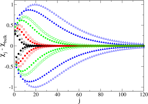
As might be expected, the boundary induces Friedel-like oscillations which become larger with decreasing temperature. Interestingly, at low temperatures the oscillations first increase and reach a maximum, before decaying at large distances. This phenomenon has been first studied by Eggert and Affleck in [34] and we will rederive their field theory result as a special case of our more general considerations in section 3.
Next, we consider the boundary susceptibility which we can easily obtain from the susceptibility profile using Eq. (1.4). The result is shown in Fig. 3.
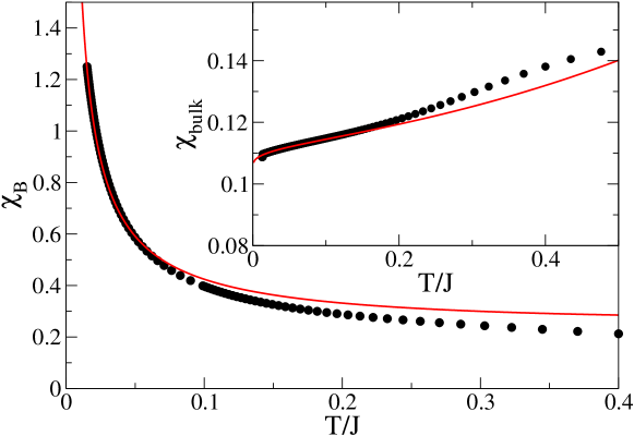
At low temperatures it was shown analytically that with a known constant [18, 19, 17]. The bulk susceptibility, on the other hand, behaves as [12], i.e., it goes to finite value at with infinite slope. We will come back to this in section 3 but already notice that the numerical data are well described by the field theory.
Finally, we also have calculated susceptibility profiles for the cases of coupled chains shown in Fig. 1(b) and (c). A ladder-like coupling of neighboring chains is, for example, realized in Sr2CuO3 [1]. In Fig. 4 it is shown that in this case an impurity in one chain also has a significant effect on a neighboring chain without impurities. The Friedel-like oscillations are reflected in the impurity-free chain due to the interchain couplings.
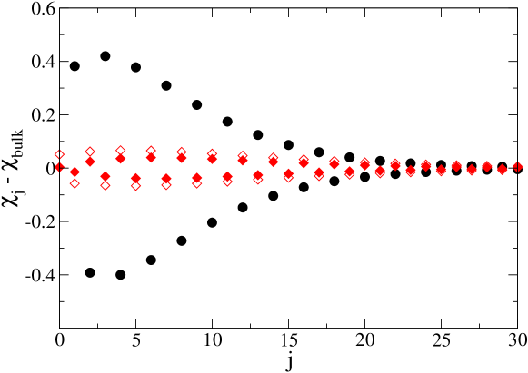
Clearly, the size of the reflected Friedel-like oscillations will depend on the ratio . However, this ratio is not the only relevant factor. The geometry of the interchain couplings plays an important role as well. In SrCuO2 neighboring chains are coupled by a ferromagnetic zigzag-type coupling. In this case an impurity in one chain leaves a neighboring chain almost unaffected even if the temperature as is shown in Fig. 5.
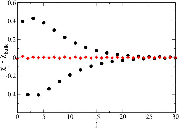
In section 5 we will show that these differences can be easily understood if one starts from the field theory results for a single chain derived in the next section and takes the interchain couplings into account perturbatively.
3 Field theory for finite spin chains
In the limit of low temperatures and large chain length, the XXZ model (1.1) can be represented by a field theory. The main step is a linearization of the dispersion around the two Fermi points. A certain linear combination of particle-hole excitations around a Fermi point then constitutes a collective bosonic mode described by the Luttinger liquid Hamiltonian
| (3.1) |
where is the spin velocity, , and the lattice constant. The bosonic field obeys the standard commutation rule with . The Luttinger parameter is a function of the anisotropy and can be determined exactly by Bethe ansatz with at the isotropic point. The spin operators can be directly expressed in terms of the boson , in particular, we have
| (3.2) |
at zero magnetic field. Here is an amplitude which can also be obtained exactly [35, 36, 37]. The separation of into a uniform and a staggered part at low energies can be understood as follows. In the equivalent spinless fermion representation of the XXZ model, obtained by a Jordan-Wigner transformation, the operator becomes the density operator. Due to the linearization of the dispersion the electrons can live either at the same Fermi point and have therefore small momentum or they can be situated at different Fermi points in which case the associated momentum is . Zero magnetic field corresponds to half-filling for the spinless fermions thus and we obtain the staggered contribution in (3.2). This also means that the local susceptibility defined in Eq. (1.2) can be separated at low temperatures into a uniform and a staggered part
| (3.3) |
In a bulk susceptibility measurement the staggered part does not contribute. This part is, however, measurable in probes of the local magnetism as for example in NMR. We will come back to this point in section 5.
If one is only interested in correlation functions for infinite system size at finite temperatures or correlation functions for finite systems at zero temperature, one can make use of the conformal invariance of the field theory. It is then sufficient to calculate the correlation at zero temperature and infinite system size and use a conformal mapping from the complex plane onto a cylinder with the circumference corresponding either to inverse temperature or system size. Here, we are, however, interested in the thermodynamics of finite chains and we will therefore have to use an explicit mode expansion
| (3.4) |
which incorporates the OBCs. Here is a bosonic annihilation operator. Eq. (3.4) is a discrete version of the mode expansions used in [13, 16] with becoming a continuous coordinate for , with fixed. Using this mode expansion, the local observables respect the discrete lattice symmetry corresponding to a reflection at the central bond (site) for even (odd), respectively. The sites and are added to model (1.1) and we demand that the spin density vanishes at these sites. Therefore the upper boundary for the integrals in (3.1) is . The zero mode part (first two terms of Eq. (3.4)) fulfills and the oscillator part (last term of Eq. (3.4)) vanishes for as required.
For the free boson model the uniform part of the susceptibility can easily be calculated and is given by [13]
| (3.5) |
Here is the elliptic theta function of the third kind for integer (even ) and of the second kind for half-integer (odd ). Note, that has a simple scaling form as a function of . The lattice parameter appears here due to the OBCs. It leads to a boundary correction which we will consider later. First, we set in (3.5) and concentrate the following limiting cases
| (3.9) |
The Curie-like divergence for odd is caused by the degeneracy of the ground state . At low temperatures the whole chain therefore behaves like a single spin. For even, on the other hand, the ground state is a singlet, . At low temperatures the chain becomes locked in this state leading to an exponentially small susceptibility. In the thermodynamic limit, , the susceptibility within the free boson approximation is just a constant.
The staggered part of the susceptibility, , for a finite chain with OBCs has been calculated in [37]. It is given by
| (3.10) |
Here is the Dedekind eta-function and the elliptic theta-function of the first kind. The summation index runs over all integers (half-integers) for even (odd), respectively. In the thermodynamic limit, , we can simplify our result and obtain
| (3.11) |
with . This agrees for the isotropic Heisenberg case, , with the result in [34]. The amplitude , first introduced in Eq. (3.2), can be determined with the help of the Bethe ansatz along the lines of Ref. [36]. This leads to with as given in Eq. (4.3) of [36]. The formulas (3.10) and (3.11) are therefore parameter free.
To find the boundary contributions, as for example the boundary free energy defined in Eq. (1.3), one has to go beyond the free boson model (3.1). When deriving the low-energy effective theory for the XXZ model, one finds in addition to the free boson model (3.1) infinitely many irrelevant terms. These terms either stem from band curvature (corrections to the linear dispersions around the Fermi points) or from the interaction term. For close to the leading irrelevant term is given by
| (3.12) |
It is the bosonized version of Umklapp scattering where two left moving electrons get scattered to right movers or vice versa interchanging a reciprocal lattice vector. This term becomes relevant for and is responsible for the opening of an excitation gap in this regime. For the isotropic case, , Umklapp scattering is marginally irrelevant and leads to important corrections to the results obtained for the free boson model. Due to the integrability of the XXZ model the amplitude of the Umklapp term can be obtained exactly as well [38]. In Ref. [16, 17] the free energy and the susceptibility corrections to the free boson result to first order in the Umklapp scattering have been calculated. For the susceptibility the following correction was obtained
| (3.13) |
with
| (3.14) |
In addition, there is also the boundary correction related to the parameter in (3.5). Expanding in this parameter to lowest order we find
| (3.15) |
where
| (3.16) |
plays the role of a lattice constant and its value can be determined for () by the Bethe ansatz and is given by [20, 21]
| (3.17) |
The uniform part of the susceptibility of a finite chain is therefore given by . The corrections to the uniform zeroth order susceptibility are important here because in the thermodynamic limit they give the boundary susceptibility . In this limit and therefore
| (3.18) |
This is just a constant contribution to the boundary susceptibility. Much more important is the boundary contribution stemming from . Here we find
| (3.19) |
with , , and being the digamma function. Note that for () the boundary spin susceptibility shows a divergent behavior as temperature decreases.
3.1 The isotropic point
At the isotropic point Umklapp scattering becomes marginal and simple perturbation theory is no longer sufficient. In this case we have to replace the Umklapp scattering amplitude by a running coupling constant which obeys a known set of renormalization group equations [38]
| (3.20) |
Here is Euler’s constant and for the isotropic case considered here, the spin velocity is . The uniform susceptibility is then given by
| (3.21) |
where in the exponentials of (3.5) and in (3.13). In this case the parameter in (3.5) is not determined by (3.17) and has to be used as a fitting parameter.
In the thermodynamic limit we can again split the susceptibility (3.21) into a bulk and a boundary part. For the bulk susceptibility this yields the result first derived by Lukyanov [38]
| (3.22) |
Here we have also added the correction from Umklapp scattering as well as a -term which stems from irrelevant operators with scaling dimension describing band curvature. The running coupling constant is given by (3.20) with . In the inset of Fig. 3 this formula is displayed in comparison to the numerical results. For the boundary susceptibility, on the other hand, we find
| (3.23) |
where we included second order corrections in as derived in [17]. The comparison of this formula with and numerical results is shown in the main panel of Fig. 3.
Finally, also the result for the staggered part of the susceptibility given in Eq. (3.10) has to be modified at the isotropic point. Here we find [37]
| (3.24) |
Now the running coupling constant also depends on the distance of site from the boundary and is given by
| (3.25) |
where the constant is not known and has to be used as a fitting parameter. Note, however, that for low temperatures and the value of becomes irrelevant and our result for therefore again parameter-free. If we consider the thermodynamic limit of Eq. (3.24) we find
| (3.26) |
A comparison of this formula with numerical data is shown in Fig. 2. The agreement is good but not perfect. The main problem here is that the temperature and the length scale set by the distance from the boundary are competing. The renormalization group equations, however, cannot be solved with both scales present. The formula (3.25) is derived in the limit when only one of those scales matter and the corrections can be significant if this is not the case.
4 The averaged susceptibility and a comparison with experimental data
In an actual crystal we have imperfections and impurities which limit the length of a spin chain segment. It is important to emphasize again that any weakening of a link is a relevant perturbation in the renormalization group sense. It is therefore expected to be a good approximation to assume that at low temperatures we have spin chain segments with open boundary conditions. As long as we do not know in detail how these defects are distributed it seems to be reasonable to assume a Poisson distribution, i.e., the probability of having an impurity at site is not influenced by the other impurities. We might, however, expect this assumption to break down for large impurity concentrations where some sort of impurity order might set in. Using a Poisson distribution we have a normalized probability to find a chain segment with sites if the impurity concentration is . Any measurement then corresponds to taking an average over this ensemble of chain segments. For the susceptibility, for example, we find
| (4.1) |
Note that in a bulk measurement only the uniform part of the susceptibility contributes. The staggered part cancels out. Using the formula (3.21) we can immediately calculate the average susceptibility . It is, however, very useful and instructive to derive a much simpler approximate formula. To this end, we notice that we have two different regimes for a finite spin chain. If the temperature is larger than the finite size gap, , we can approximate . If, one the other hand, we expect to see more or less the ground state properties of the finite chain. This means, according to Eq. (3.9), that there will be no contribution when the chain length is even while if the chain length is odd. We can therefore introduce a length where this crossover occurs. Here is a parameter which we expect to be of order . For the average susceptibility we can therefore write
An interesting experiment has been performed by Kojima et al. [5] where Palladium has been doped into the spin chain compound Sr2CuO3. The Pd ions then replace the Cu ions, act as non-magnetic impurities, and cut the chain into finite segments. A complication in the analysis of this experiment occurs because even the undoped Sr2CuO3 samples already have a substantial amount of chain breaks. It is believed that this is mainly a consequence of excess oxygen, i.e., we are in reality dealing with Sr2CuO3+δ. In a simple picture, an excess oxygen ion pulls two electrons out of the copper chain. If these holes are relatively immobile this also corresponds to a chain break. In the comparison of the experimental data for Sr2Cu1-xPdxO3+δ and formula (4) shown in Fig. 6 we therefore use as an effective impurity concentration incorporating both the chain breaks due to excess oxygen and due to the non-magnetic Pd ions.
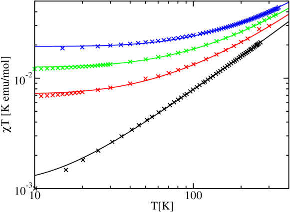
Furthermore, we have subtracted a constant contribution from the experimental data which is expected to be present due to core diamagnetism and Van Vleck paramagnetism. The values for and which yield the best fit of the experimental data are shown in table 1.
| (Exp.) | (Theory) | [emu/mol] |
|---|---|---|
For Pd concentrations of and the obtained values for are consistent with the picture of having a certain amount of chain breaks due to excess oxygen already in the undoped compound. For , however, this picture seems to fail. Reasons for this could be either on the experimental side (perhaps not all Pd ions really go into the sample, or some go in interstitially) or in the theoretical description. If, for example, the Pd ions tend to cluster above a certain concentration, then our assumption of a Poisson distribution becomes incorrect.
5 The Knight shift and the role of interchain couplings
As already mentioned, the staggered part of the susceptibility cannot be observed in a bulk measurement. This, however, is possible by NMR because here the resonance frequency gets shifted by the local magnetic field. This so-called Knight shift can therefore be directly related to the local susceptibility. For a chain of length it is given by
| (5.1) |
where () is the electron (nuclear) gyromagnetic ratio, respectively and the hyperfine coupling tensor. It is usually sufficient to take only and into account because of the short-range nature of the hyperfine interaction.
To compare with experiment, we assume again a Poisson distribution of chain breaks so that the measured Knight shift is given by an average over all possible chain lengths. Furthermore, each site in a chain of length gives a different Knight shift according to (5.1). If we assume that each of these Knight shifts has a Lorentzian lineshape with width we find for the NMR spectrum
| (5.2) |
Using the results for the uniform (3.21) and the staggered part (3.24) we can now immediately calculate the NMR spectrum for an ensemble of isotropic Heisenberg chain segments and compare to experimental data for Sr2CuO3 obtained by Takigawa et al. [6, 7]. We use K as exchange constant in (1.1) and hyperfine coupling constants T, T, and T [39]. Here the index denotes the magnetic field direction. We calculate the spectrum as a function of and use T. For the resonance field MHz used in the experiment [6] this is consistent with where MHz/T [40]. A comparison of formula (5.2) for this set of material-dependent parameters with experiment is shown in Fig. 7.
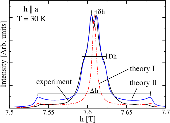
Here the impurity concentration and the Lorentzian linewidth have been used as fitting parameters. Note that the sample used for the NMR experiment has been annealed thus dramatically reducing the amount of excess oxygen and the associated chain breaks compared to the sample used for the susceptibility measurement shown in Fig. 6. The theory predicts a central peak corresponding to the bulk susceptibility value and two shoulders with separation (see curve ’theory I’ in Fig. 7) which are caused by the maxima of the local susceptibility (see, for example, Fig. 2). Theoretically, we find that , i.e., the separation of the shoulders increases with decreasing temperature. This is in agreement with experimental findings [6]. The central peak, however, has a much more complex structure than predicted. The peak is split (feature in Fig. 7) and has prominent shoulders (feature in Fig. 7). These features are only observed in experiment at temperatures K, whereas at higher temperatures the theoretical prediction agrees well with experimental data (not shown).
To explain the additional features in the NMR spectra at K we have to take the interchain coupling into account. Sr2CuO3 shows three-dimensional Néel ordering at K. According to the usual chain mean field argument the interchain coupling should therefore also be of order K. This estimate is consistent with band structure calculations [8]. As we have already demonstrated numerically in Fig. 4, a ladder-like interchain coupling as present in Sr2CuO3 leads to a reflection of susceptibility oscillations. Therefore another typical Knight shift is expected to be present in the NMR spectra, related to the maxima of the reflected oscillations. As long as we can calculate this effect perturbatively. Starting from the definition of the local susceptibility given in Eq. (1.2) we obtain to first order
| (5.3) |
Here, the lower index stands for the infinitely long chain without chain breaks whereas the lower index denotes the chain with a chain break at site . Both, the two-point correlation and the local susceptibility have a uniform and a staggered part in the low temperature limit. We therefore find with and
| (5.4) |
Here Eq. (3.11) has to be used for while is the staggered part of the bulk two-point correlation function. In Fig. 4, formula (5.4) is compared with the numerical result and good agreement is found.
If we take these reflections into account, then also the additional features in the NMR spectra are explained as shown in Fig. 7 (curve ’theory II’). In particular, the shoulders with separation directly correspond to the maxima of the reflected susceptibility oscillations. The splitting of the peak is of different origin. It is in fact not a splitting but rather a loss of intensity at the value which corresponds to the bulk susceptibility. The oscillations and reflected oscillations spread over the entire crystal at low temperatures so that there are simply no sites left which show bulk behavior. Rather interestingly, the peak usually associated with the bulk susceptibility value therefore turns into a dip at low temperatures due to the presence of chain breaks and interchain couplings.
Finally, we also want to shed some light on the role played by the geometry of the interchain couplings. To this end, we consider an interchain coupling as shown in Fig. 1(c). Such a coupling is realized in SrCuO2 with a ferromagnetic [1, 8]. Using again first order perturbation theory we find in this case
| (5.5) |
Separating this into a uniform and a staggered part we find and
| (5.6) |
Therefore no reflections will occur in this case to first order in perturbation theory consistent with the numerical results shown in Fig. 5. This also means that an NMR spectrum for SrCuO2 would not show any shoulders associated with the coupling to the nearest neighbor chain. Reflections in chains further away might, however, be still possible which then would again lead to additional structures in the NMR spectra at low temperatures.
6 Summary and Conclusions
We have investigated here how chain breaks and interchain couplings affect the physical properties of spin chain compounds. A weak coupling of two Heisenberg chains is an irrelevant perturbation in the renormalization group sense whereas the weakening of a bond in an otherwise homogenous chain is relevant. Open boundary conditions are therefore the stable fix point. Due to this reasoning it is expected that a wide class of perturbations like impurities or dislocations present in any real compound can be effectively described at low energies as a chain break. An experimental measurement then corresponds to taking an average over an ensemble of finite chain segments with open boundaries.
By combining a low-energy effective field theory with Bethe ansatz we have derived parameter-free formulas for the thermodynamics of finite spin- Heisenberg chains with open boundary conditions. Particular emphasis was put on a calculation of the susceptibility. Due to the broken translational invariance there exists a site-dependent staggered susceptibility in addition to the uniform site-independent part. However, even the uniform part is affected by the open boundary conditions in the sense that a surface contribution arises which is not present for periodic boundary conditions.
We have shown that susceptibility measurements on Sr2CuO3 doped with non-magnetic Pd ions are well described by the theory presented here. One of the complications arising for this compound is, however, that even the undoped sample apparently already has a relatively large amount of chain breaks which are believed to be caused by excess oxygen. The impurity concentration used in the theory to fit the experimental data therefore differs significantly from the nominal Pd concentration. The emerging picture nevertheless seems to be consistent - at least at low impurity concentrations - with a fixed concentration of additional chain breaks already present in the undoped sample. It would certainly be of some value to obtain experimental data for this or some other spin-chain compound where the impurity concentration is well controlled and a direct comparison with theory therefore possible.
Furthermore, we used the field theory to calculate NMR spectra. Importantly, the Knight shift is proportional to the local susceptibility so that the staggered site-dependent part of the susceptibility, which cannot be observed in a bulk susceptibility measurement, becomes observable. As has already been shown previously [6], the staggered susceptibility leads to a broad background in the NMR spectra with edges caused by the maxima of the staggered susceptibility. For Sr2CuO3 it has, however been found that the NMR spectra at low temperatures show puzzling additional features which have been ascribed in [7] to a coupling to phonons. Here we have shown that these features quite naturally arise in a spin-only model if the known interchain couplings are taken into account. It is also important to note that the geometry of the interchain couplings is crucial. As a specific example we considered in addition to the ladder-like interchain coupling relevant for Sr2CuO3 also the zigzag-like interchain coupling realized in SrCuO2. In the latter case no additional structures in the NMR spectra related to this interchain coupling will occur. NMR experiments on spin chain compounds are therefore not only helpful to study impurity effects, they can also be used to investigate the geometry and strength of interchain couplings.
Acknowledgments
I want to thank all my collaborators on this and related topics, in particular, Ian Affleck, Michael Bortz, Sebastian Eggert, Andreas Klümper, and Nicolas Laflorencie.
References
- 1. Motoyama N., Eisaki H., Uchida S., Phys. Rev. Lett., 1996, 76, 3212.
- 2. Pratt F.L., Blundell S.J., Lancaster T., Baines C., Takagi S., Phys. Rev. Lett., 2006, 96, 247203.
- 3. Thurber K.R., Hunt A.W., Imai T., Chou F.C., Phys. Rev. Lett., 2001, 87, 247202.
- 4. Sologubenko A.V., Giannó K., Ott H.R., Vietkine A., Revcolevschi A., Phys. Rev. B, 2001, 64, 054412.
- 5. Kojima K., et al., Phys. Rev. B, 2004, 70, 094402.
- 6. Takigawa M., Motoyama N., Eisaki H., Uchida S., Phys. Rev. B, 1997, 55, 14129.
- 7. Boucher J.P., Takigawa M., Phys. Rev. B, 2000, 62, 367.
- 8. Rosner H., Eschrig H., Hayn R., Drechsler S.L., Málek J., Phys. Rev. B, 1997, 56, 3402.
- 9. Hase M., Phys. Rev. Lett., 1993, 70, 3651.
- 10. Ma S., Broholm C., Reich D.H., Sternlieb B.J., Erwin R.W., Phys. Rev. Lett., 1992, 69, 3571.
- 11. Rüegg C., et al., Phys. Rev. Lett., 2008, 101, 247202.
- 12. Eggert S., Affleck I., Takahashi M., Phys. Rev. Lett., 1994, 73, 332.
- 13. Eggert S., Affleck I., Phys. Rev. B, 1992, 46, 10866.
- 14. Giamarchi T., Quantum physics in One Dimension (Clarendon Press, Oxford, 2004).
- 15. Zotos X., Naef F., Prelovšek P., Phys. Rev. B, 1997, 55, 11029.
- 16. Sirker J., Laflorencie N., Fujimoto S., Eggert S., Affleck I., Phys. Rev. Lett., 2007, 98, 137205.
- 17. Sirker J., Laflorencie N., Fujimoto S., Eggert S., Affleck I., J. Stat. Mech., 2008, P02015.
- 18. Fujimoto S., Eggert S., Phys. Rev. Lett., 2004, 92, 037206.
- 19. Furusaki A., Hikihara T., Phys. Rev. B, 2004, 69, 094429.
- 20. Bortz M., Sirker J., J. Phys. A: Math. Gen., 2005, 38, 5957.
- 21. Sirker J., Bortz M., J. Stat. Mech., 2006, P01007.
- 22. Sirker J., Bortz M., Phys. Rev. B, 2006, 73, 1.
- 23. Bursill R., et al., J. Phys: Cond. Mat., 1995, 7, 8605.
- 24. Wang X., Xiang T., Phys. Rev. B, 1997, 56, 5061.
- 25. Shibata N., J. Phys. Soc. Jpn., 1997, 66, 2221.
- 26. Sirker J., Klümper A., Phys. Rev. B, 2002, 66, 245102.
- 27. Sirker J., Klümper A., Europhys. Lett., 2002, 60, 262.
- 28. Sirker J., Klümper A., Phys. Rev. B, 2005, 71, 241101(R).
- 29. Trotter H.F., Proc. Amer. Math. Soc., 1959, 10, 545.
- 30. Suzuki M., Commun. Math. Phys., 1976, 51, 183.
- 31. Suzuki M., Phys. Rev. B, 1985, 31, 2957.
- 32. Eggert S., Rommer S., Phys. Rev. Lett., 1998, 81, 1690.
- 33. Klümper A., Raupach R., Schönfeld F., Phys. Rev. B, 1999, 59, 3612.
- 34. Eggert S., Affleck I., Phys. Rev. Lett., 1995, 75, 934.
- 35. Affleck I., J. Phys. A, 1998, 31, 4573.
- 36. Lukyanov S., Terras V., Nucl. Phys. B, 2003, 654, 323.
- 37. Sirker J., Laflorencie N., arXiv:0811.2106, 2008.
- 38. Lukyanov S., Nucl. Phys. B, 1998, 522, 533.
- 39. Monien H., Pines D., Takigawa M., Phys. Rev. B, 1990, 43, 258.
- 40. Abragam A., Bleaney B., Electron Paramagnetic Resonance of Transition Ions (Clarendon Press, Oxford 1970).