Spitzer-IRS Study of the Antennae Galaxies NGC 4038/39

Abstract

Using the Infrared Spectrograph on the Spitzer Space Telescope, we observed the Antennae galaxies obtaining spectral maps of the entire central region and high signal-to-noise $5-38\mu$m spectra of the two galactic nuclei and six infrared-luminous regions.

The total infrared luminosity of our six IR peaks plus the two nuclei is $L_{\rm IR}=3.8\cdot 10^{10}$ L_⊙, with their derived star formation rates ranging between 0.2 and 2 M_⊙/yr, with a total of 6.6 M_⊙/yr. None of the typical mid-infrared tracers of AGN activity is detected in either nucleus of the system, excluding the presence of an dust enshrouded accretion disk. The hardest and most luminous radiation originates from two compact clusters in the southern part of the overlap region, which also have the highest dust temperatures. PAH emission and other tracers of softer radiation are spatially extended throughout and beyond the overlap region, but regions with harder and intenser radiation field show a reduced PAH strength.

The strong H₂ emission is rather confined around the nucleus of NGC 4039, where shocks appear to be the dominant excitation mechanism, and the southern part of the overlap region, where it traces the most recent starburst activity. The luminosity ratio between the warm molecular gas (traced by the H₂ lines) and the total far-IR emission is $\sim 1.6\cdot 10^{-4}$, similar to that found in many starburst and ULIRGs. The total mass of warm H₂ in the Antennae is $2.5\cdot 10^{7}$ M_⊙, with a fraction of warm to total H₂ gas mass of about 0.35%. The average warm H₂ temperature is $302\pm 26$ K and appears anti-correlated with the radiation field hardness, possibly due to an evolution of the PDR morphology. The previously reported tight correlation between the H₂ and PAH emission was not found but higher total PAH emission to continuum ratios were found in PDRs with warmer gas.

1. Introduction

The Antennae galaxies, NGC 4038/39 (Arp 244), are arguably the best-known example of interacting galaxies. The two galactic nuclei of NGC 4038 and NGC 4039, and the dust-obscured overlap region in between, exhibit one of the most stunning examples of starburst activity in the nearby Universe. They are the first system in the Toomre (1977) merger sequence. In the Antennae we observe the symmetric encounter between two normal Sc type spirals at an early merger stage (Mihos & Hernquist, 1996).

From the four IRAS bands Sanders et al. (2003) derived total infrared luminosities of $\log L_{\rm FIR}=L_{40-400\mu m}=10.73$ and $\log L_{\rm IR}=L_{8-1000\mu m}=10.84$, corresponding to $L_{\rm FIR}=5.6\cdot 10^{10}$ L_⊙ and $L_{\rm IR}=7.2\cdot 10^{10}$ L_⊙ for a distance of 22 Mpc. With a luminosity just below $10^{11}$ L_⊙ the Antennae does not classify as a luminous infrared galaxy (LIRG).

The distance to the Antennae has been a subject of recent controversy. Earlier estimates by Wilson et al. (2000); Gao et al. (2001) found 20 Mpc, and Whitmore et al. (1999) determined 19.2 Mpc. However, using HST-ACS Saviane et al. (2008) observed the tip of the red giant branch of the stellar populations in the southern tail of the Antennae, and determined a distance of only $13.3\pm 1.0$ Mpc. This estimate was soon again altered when, recently, Schweizer et al. (2008) derived $22.3\pm 2.8$ Mpc from the type Ia supernova 2007sr light curve, much closer to the old estimates, which were mainly based on the Hubble flow. Schweizer et al. (2008) also re-analyzed the HST-ACS data and identified a different location of the tip of the red giant branch, which agreed with their SN1a distance. Combining three independent methods Schweizer et al. (2008) determined a distance of $22\pm 3.0$ Mpc, which is the distance we assume throughout this paper.

The first deep optical images of the Antennae taken with the Wide Field Camera on HST revealed over 700 point-like objects (Whitmore & Schweizer, 1995). Subsequent V-band observations with WFPC2 increased the sensitivity by three magnitudes and revealed between 800 and 8000 clusters in four age ranges (Whitmore et al., 1999). These and related observations at optical and near-IR wavelengths (e.g., Fritze-v. Alvensleben, 1999; Whitmore & Zhang, 2002; Kassin et al., 2003; Brandl et al., 2005; Mengel et al., 2005; Fall et al., 2005; Bastian et al., 2006) started extensive studies of the properties of extragalactic star clusters in a statistically significant way. The Antennae provide an excellent environment to study the transformation of supergiant molecular clouds (SGMCs) into super star clusters (SSCs) (de La Fuente Marcos & de La Fuente Marcos, 2006) and their further dynamical evolution (Whitmore et al., 1999; Fall et al., 2005; Bastian et al., 2006; Anders et al., 2007; Whitmore et al., 2007). Numerous other studies (Gilbert et al., 2000; Mengel et al., 2001, 2002; Gilbert & Graham, 2007) focused on detailed investigations of a few individual SSCs via means of near-IR spectroscopy.

The first high signal-to-noise mid-IR images of the Antennae were made by the Infrared Space Observatory ISO. ISOCAM observations at angular resolutions of $5-8^{\prime\prime}$ showed that the overlap region contributes more than half of the total luminosity observed in the $12.5-18\mu$m range (Vigroux et al., 1996). The comparison between HST and ISOCAM images revealed a compact, optically-obscured knot which produces 15% of the total $12.5-18\mu$m luminosity (Mirabel et al., 1998). Further ISO studies were performed by Kunze et al. (1996); Fischer et al. (1996); Klaas et al. (1997) and Haas et al. (2005) followed by Spitzer-IRAC $3-8\mu$m observations (Wang et al., 2004). Recent sub-arcsecond imaging and N-band spectroscopy with VLT-VISIR resolved the Hii region / PDR interface and revealed a highly obscured SSC that does not have an optical or near-IR counterpart (Snijders et al., 2006).

Observations at the longer far-infrared, sub-millimeter and radio wavelengths generally agree with the mid-IR picture. The early works of Hummel & van der Hulst (1986) with the VLA at 1.465 GHz and 4.885 GHz found thermal radio knots, which account for about 35% of the total emission, coinciding with peaks in H_α emission associated with recent star formation. The high resolution radio maps with the VLA (Neff & Ulvestad, 2000) at 6 and 4 cm became the basis for many subsequent studies. Nikola et al. (1998) mapped the Antennae in the [C II] cooling line associated with photo-dissociation regions at an angular resolution of $55^{\prime\prime}$ and found that the starburst activity is confined to small regions of high star formation efficiency. Wilson et al. (2000, 2003) found an excellent correlation between the strengths of the CO emission and the $15\mu$m broad band emission seen by ISO, and determined masses of $(3-6)\cdot 10^{8}$ M_⊙ for the largest molecular complexes, typically an order of magnitude larger than the largest structures found in the disks of more quiescent spiral galaxies. The total molecular gas mass in the overlap region is $1.2\cdot 10^{9}$ M_⊙ (Stanford et al., 1990) – several times higher than the amount of gas in the two nuclei – while the molecular gas mass for the entire Antennae system is $1.5\cdot 10^{10}$ M_⊙ (Gao et al., 2001). At a star formation rate (SFR) of $\sim 20$ M_⊙ yr^-1 (Zhang, Fall & Whitmore, 2001), the gas consumption timescale is only 700 Myr. Gao et al. (2001) also estimated a “normal” star formation efficiency (SFE) over the entire Antennae system of $L_{\rm IR}/M_{H_{2}}\sim 4.2$ L_⊙/ M_⊙, which is similar to that of GMCs in the Galactic disk. Schulz et al. (2007) combined ¹²CO (1-0), (2-1), (3-2) and $870\mu$m maps with data from X-ray to radio and PDR models, and found that the clouds have dense ($4\times 10^{4}cm^{-3}$) cores and low kinetic temperatures ($\leq 25$ K), showing no signs of intense starburst activity.

Finally, numerous X-ray observations, predominantly with Chandra, have revealed many X-ray sources, including several long-term variable, ultra-luminous X-ray (ULX) sources (Zezas et al., 2002a, 2006). Although most ULXs are likely black hole/high mass X-ray binaries accreting via Roche lobe overflow, Feng & Kaaret (2006) have argued that the most luminous ULX, X-16, is a candidate for an intermediate mass black hole (IMBH), while Zezas et al. (2007) note that its X-ray luminosity could be produced by a $\sim 80$ M_⊙ black hole accreting at the Eddington limit. From the spatial distribution of the infrared counterparts to the ULXs, Clark et al. (2007) concluded that they mainly trace the recent star formation history. Baldi et al. (2006a) studied metal abundances in the hot interstellar medium and found variations from 0.2 Z_⊙ to $20-30$ Z_⊙, but found no correlation between the radio/optical star formation indicators and metallicity (Baldi et al., 2006b).

In this paper we study the central region of the Antennae galaxies based on spatially resolved mid-IR spectroscopy. Our aim is to characterize the starburst activity in general, the super star clusters in particular, and their interplay (heating and ionization) with the interstellar medium. From the mid-infrared spectra we derive a total infrared luminosity for each of our six star forming peaks. These luminosities are used to estimate the star formation rates. Particular attention will be given to the H₂ rotational lines, which probe the warm component of molecular hydrogen and which will be used to derive the gas masses and temperatures. The outline of this paper is as follows: In the next section we describe the observations along with the data reduction and calibration. Section 3 discusses how the spectral features have been measured and the key parameters were derived, and section 4 presents the results, both on individual clusters and on the central region as a whole, followed by the summary.

2. Observations and Data Reduction

We used the Infrared Spectrograph (IRS) (Houck et al., 2004) on board the Spitzer Space Telescope (Werner et al., 2004) to observe the central interaction region of the Antennae galaxies at unprecedented depth. The IRS observations of the Antennae are part of a guaranteed time program (PI Houck, Spitzer PID 21) on the spectroscopic study of star formation in interacting galaxies. The observing parameters are listed in Table 1 and described in more detail in Sections 2.1 and 2.2.

Table 1Observing Parameters

	‘hires’	‘lores’
Obs.date	3 Jan 2005	3 Jul 2005
		12 Jul 2005
		23 Jan 2006
AOR-keys	3842304	3841536
	3842560	3841792
		16707840
		16708096
		16708352
$t_{int}$	$24\times 30$s (SH)	$2\times 14$s (SL)
	$10\times 60$s (LH)	$2\times 14$s (LL)
Slit sizes	$4.\!^{\prime\prime}7\times 11.\!^{\prime\prime}3$ (SH)	$3.\!^{\prime\prime}6\times 57^{\prime\prime}$ (SL)
	$11.\!^{\prime\prime}1\times 22.\!^{\prime\prime}3$ (LH)	$10.\!^{\prime\prime}5\times 168^{\prime\prime}$ (LL)

2.1. ‘Hires’ Observations

We have made observations in IRS high resolution (‘hires’) mode at $R=600$ with the Short-High (SH) [$9.9-19.6\mu$m] and Long-High (LH) [$18.7-37.2\mu$m] modules. The angular slit sizes are listed Table 1 and correspond to approximately $500\times 1200$ pc² (SH) and $1200\times 2380$ pc² (LH) at the distance of the Antennae.

The spectra from the IRS ‘hires’ modules were taken with a standard staring mode Astronomical Observing Template (AOT), producing two exposures per ‘cycle’ at separate nod positions along the slit. The coordinates of the eight observed regions within NGC 4038/39 are listed in Table 2 and the slit positions are illustrated in Fig. 1. We note that the IRS position of the nucleus of NGC 4038 does not exactly coincide with the radio nucleus but is slightly shifted toward the north to also include the nearby, active star forming region.

Table 2Parameters of the Pointed Observations with Cluster Designations from the Literature

Name	RA (J2000)	Dec (J2000)	LH SF	WS95	W99	WZ02	B05	N00
nucleus 4038	12 01 53.01	-18 52 02.7	0.77
nucleus 4039	12 01 53.54	-18 53 10.2	0.63
peak 1	12 01 54.98	-18 53 05.7	0.65	80	$\cdots$	3	157	2-1
peak 2	12 01 54.58	-18 53 03.4	0.56	86(89/90)	11/9/14/30/33/39	5	136	2-6
peak 3	12 01 55.39	-18 52 48.9	0.50	119/120(/117)	19/17	7	176	4-2
peak 4	12 01 50.42	-18 52 12.6	0.59	405	2	25	$\cdots$	11-2
peak 5	12 01 54.75	-18 52 51.1	0.45	115	$\cdots$	$\cdots$	148	3-5
peak 6	12 01 54.80	-18 52 13.5	0.56	384/382/389	18	24	154	5-5
reference sky	12 01 49.00	-18 52 50.0

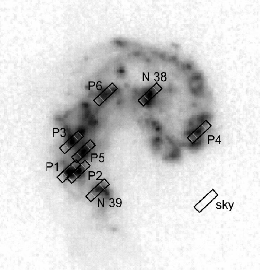
Figure 1.— Illustration of the IRS SH slit positions for the given observing date, over-plotted on the IRAC $8\mu$m map (Wang et al., 2004) of the Antennae. North is toward the upper right.

The data were pre-processed by the Spitzer Science Center data reduction pipeline version 13.2 (Observer’s Manual, 2004). To avoid uncertainties introduced by the flat-fielding in earlier versions of the automated pipeline processing, we started from the two-dimensional, unflat-fielded data products. These products are part of the “basic calibrated data” (BCD) package provided by the Spitzer Science Center.

First, all images were cleaned of bad pixels using the IDL procedure IRSCLEAN with a ‘Maskval=128’. The various 2-dimensional spectra from the same nod position were median-combined within the Spectral Modelling, Analysis, and Reduction Tool (SMART) version 5.5.1. (Higdon et al., 2004). A median ‘sky’ spectrum was computed from both nods of the sky position (#9) and subtracted from each median nod image. The spectral extraction was also done within SMART, using full aperture extraction. The ‘fluxcon’ tables were disabled by setting them to ‘s1’. Instead, the spectra were flat-fielded and flux calibrated by multiplication with the relative spectral response function (RSRF) using the IRS RSRF of the standard star $\xi$-Dra for both SH and LH spectra. We have not corrected for periodic “detector fringing” in the spectra since these artifacts have no effect on the analysis carried out in this paper.

After these steps there was a noticeable and expected mismatch between the fluxes measured by the IRS SH and LH modules at the same wavelengths. This mismatch is most likely due to extended emission, picked up by the wider LH slit. For an ideal point source there would be very little mismatch while for uniform surface brightness SH would only see 21% of the flux measured by LH. In principle there are three possibilities to match the two spectra: (i) scale LH down to match SH, (ii) scale SH up to match LH, or (iii) use a wavelength dependent scaling factor that affects both SH and LH. (i) is best if the spectrum of a compact source surrounded by extended emission is of interest, (ii) should be used to quantify the extended emission, and (iii) is arguably the best method to account for both components but requires additional assumptions. Since we are most interested in the spectral information from unresolved SSCs – which are fully covered by both SH and LH slits – we have chosen method (i). In any case, the quantitative results derived in this paper are from the lines covered by the SH module and are not affected by the scaling. The scaling factors ‘SF’ applied to the LH fluxes are listed in Table 2. The resulting IRS ‘hires’ spectra from the two nuclei and the six infrared peaks are shown in Fig. 3. The total observing time was 4.4 hours.

2.2. ‘Lores’ Observations

We have also made observations in the IRS low resolution (‘lores’) mode at $R=65-130$ with the Short-Low (SL) [$5.2-14.5\mu$m] and Long-Low (LL) [$14.0-38.0\mu$m] modules. The angular slit sizes are listed Table 1. The observations were made with both ‘lores’ modules in spectral mapping mode. The AORs were intentionally designed to make use of the facts that the sub-slits SL1 and SL2 are adjacent and record data simultaneously, and that the orientation would have changed after six months (half a solar orbit). However, an unfortunate delay of six months in the scheduling doubled the spatial offset between SL1 and SL2 instead of providing the same spatial coverage. The problem was detected and corrected by requesting another SL1 map six months later, specifically designed to fill in the missing parts. The mapped areas are illustrated in Fig. 2. The total mapping time of all observations combined was 7.1 hours.

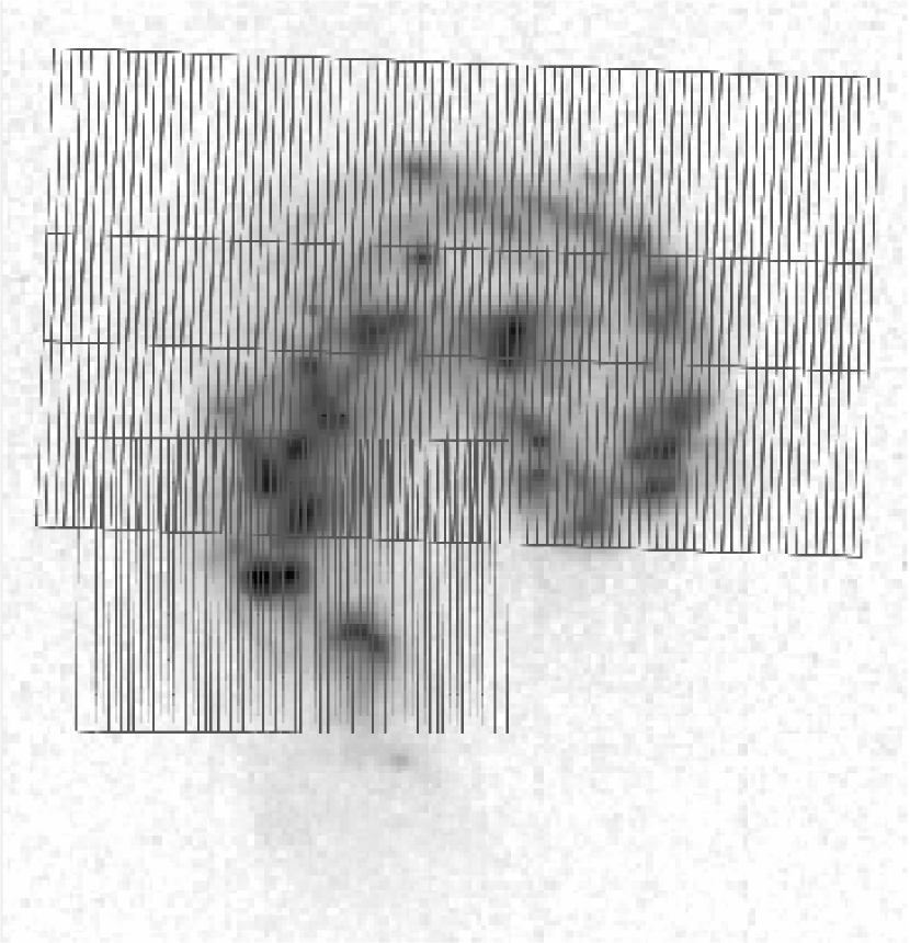
Figure 2.— Illustration of the areal coverage of the IRS SL spectral map overlaid on the IRAC $8\mu$m map. The larger part on top is the initial map while the lower, smaller area indicates the “filler” part. North is toward to upper right.

All data were processed with the standard pipeline version 13. Further reduction and analysis started from the two-dimensional, flat-fielded data products, which are part of the “basic calibrated data” package provided by the Spitzer Science Center.

Most of the reduction and spectral analysis of the large data cube has been made with CUBISM (Smith et al., 2007a). CUBISM is an IDL program developed by the SINGS Legacy team to combine slit spectra at various angles and positions and create spectral maps and local spectra. Artifacts in the resulting spectral maps were cleaned with a combination of a local noise estimate and median replacement, and the procedure IRSCLEAN, version 1.3. The latter is based on a multi-resolution analysis algorithm (Murtagh et al., 1995), where an image is subsequently smoothed to different scales, using a wavelet transform. IRSCLEAN is a contributed IRS software, which we modified slightly to use a more localized noise estimate on a sub-slit basis. We have also used Gaussian rather than uniform noise estimates. The algorithm was first tested on the “sky” spectra. Fig. 4 shows the resulting line maps for six important spectral features: the fine-structure lines of [Ne II] and [S IV], the $11.3\mu$m and $8.6\mu$m emission feature of PAHs, and the molecular hydrogen H₂ S(2) and S(3) lines.

3. Analysis

Fig. 3 reveals the spectral richness of the high signal-to-noise spectra. Important common features include the PAH emission bands, silicate absorption features, ionic fine-structure lines, atomic and molecular hydrogen lines, and the spectral continuum. In this Section we describe how the quantities relevant to our discussion have been derived from the ‘lores’ and ‘hires’ spectra. We emphasize the complementary character of the ‘lores’ and ‘hires’ data in our analysis. While the latter is used to derive accurate line fluxes the former is mainly used for a qualitative assessment of the spatial characteristics and for cross-checks with the ‘hires’ data.

Figure 3.— IRS SH+LH spectra of the two nuclei of NGC 4038 and NGC 4039 and the six infrared peaks listed in Table 2 and illustrated in Fig. 1. Most of the detected spectral lines are labeled.

3.1. Continuum Flux Densities

In order to characterize the slope of the spectral continuum we have derived the flux densities $F_{\nu}$ at two narrow wavelength intervals, namely at $14.75-15.25\mu$m and at $29.5-30.5\mu$m, here referred to as $F_{15\mu m}$ and $F_{30\mu m}$, respectively. These wavelengths have been chosen as they are not significantly affected by known emission or absorption features. Both intervals contain about 20 resolution elements, and the continuum within that narrow range is assumed to have a linear slope. The flux densities of each resolution element within the wavelength intervals have been averaged to reduce their sensitivity to noise spikes and narrow spectral features, resulting in the quasi-monochromatic flux densities $F_{15\mu m}$ and $F_{30\mu m}$.

This approach is similar to the one described in Brandl et al. (2006) and is arguably the best direct estimate of the spectral continuum. The flux measurements are listed in Table 3. The continuum fluxes will be discussed in detail in Section 4.5.

Table 3Continuum Fluxes

	$F_{15\mu m}$	$F_{30\mu m}$	$F_{15\mu m}/F_{30\mu m}$
Position	[mJy]	[mJy]
nuc 4038	103	649	0.159
nuc 4039	39	334	0.117
peak 1	383	1994	0.192
peak 2	260	1853	0.140
peak 3	79	787	0.101
peak 4	32	231	0.137
peak 5	69	699	0.099
peak 6	35	233	0.150

Note. — The flux densities listed here and in the subsequent tables are the values directly measured within the IRS SH slit aperture of $4.\!^{\prime\prime}7\times 11.\!^{\prime\prime}3$. The fluxes longward of $20\mu$m were measured with the larger IRS LH slit but have been scaled down by the scaling factors listed in Table 2.

3.2. Polycyclic Aromatic Hydrocarbons (PAHs)

The spectra in Fig. 3 show that the spectral shape at shorter wavelengths is largely dominated by the strong emission features from PAHs. The strength and equivalent width of the PAH features were measured using the IDL program PAHFIT (Smith et al., 2007b). PAHFIT decomposes the spectra into the individual contributions from starlight, thermal emission from dust, atomic and molecular emission lines, and the PAH emission bands. The latter, combined with extinction dominated by the silicate absorption bands around $9.7\mu$m and $18\mu$m, is the main application of the routine and both are treated meticulously.

We have chosen to measure the below listed PAH features from the ‘hires’ spectra rather than the ‘lores’ maps for two reasons. First, due to the longer integration times the signal-to-noise is higher than at individual positions of the spectral map. Second, all other spectral diagnostics were derived from the ‘hires’ spectra as well, and an accurate comparison does benefit from using the same slit apertures. However, since PAHFIT has been designed to analyze IRS ‘lores’ spectra and does not accurately fit narrow emission lines we removed the emission lines from the ‘hires’ spectra for the purpose of the PAH measurements. This was done by linear interpolation between the fluxes directly short-wards and long-wards of the emission lines. PAHFIT uses Drude profiles to fit 15 PAH features of different width in the IRS-SH range.

The thermal dust continuum is fitted by a combination of modified black bodies at fixed temperatures of 35, 40, 50, 90, 135, 200 and 300 Kelvin. PAHFIT can automatically correct for extinction estimated from the depth of the $9.7\mu$m silicate absorption feature. However, we have turned off this automatic feature since the ‘hires’ spectra cover only part of the $9.7\mu$m silicate absorption and we noticed that, under these conditions, extinction is being used as a free parameter to optimize fit results without strong physical motivation.

The central wavelength was fixed and the full width at half maximum (FWHM) was allowed to vary by at most 20%. Several adjacent, broad PAH features cannot be resolved and are blended into one broad complex, and we list the combined fluxes from both components. Such cases are the features at 11.23 and $11.33\mu$m, and at 12.62 and $12.69\mu$m. The PAH features at 14.04, 15.9, 18.92 and $33.1\mu$m were not included in the analysis because of their intrinsic weakness. The measured PAH fluxes and equivalent widths are listed in Table 4. The listed uncertainties include the uncertainty in the absolute flux calibration, which we estimate to be in the order of 10%, and the fit error as given by PAHFIT. Both contributions have been added in quadrature.

Table 4PAH feature strengths longward of $10\mu$m from the ‘hires’ spectra

	F10.7μm	F11.3μm	F12.0μm	F12.7μm	F13.5μm	F14.2μm	F16.5μm	F17.4μm	F17.9μm
Position	EW10.7μm	EW11.3μm	EW12.0μm	EW12.7μm	EW13.5μm	EW14.2μm	EW16.5μm	EW17.4μm	EW17.9μm
nuc 4038	$0.73\pm 0.40$	$18.02\pm 1.40$	$9.41\pm 0.65$	$14.24\pm 1.36$	$3.89\pm 0.46$	$1.20\pm 0.24$	$1.27\pm 0.20$	$6.80\pm 1.40$	$0.46\pm 0.63$
	$0.05\pm 0.01$	$1.31\pm 0.15$	$0.67\pm 0.08$	$0.97\pm 0.14$	$0.24\pm 0.04$	$0.07\pm 0.02$	$0.06\pm 0.01$	$0.29\pm 0.04$	$0.02\pm 0.01$
nuc 4039	$0.53\pm 0.09$	$9.91\pm 0.69$	$4.45\pm 0.25$	$7.17\pm 0.59$	$1.97\pm 0.18$	$6.06\pm 0.10$	$0.51\pm 0.08$	$3.53\pm 0.36$	$0.30\pm 0.10$
	$0.09\pm 0.02$	$1.70\pm 0.19$	$0.75\pm 0.09$	$1.18\pm 0.16$	$0.31\pm 0.04$	$0.09\pm 0.02$	$0.06\pm 0.01$	$0.42\pm 0.06$	$0.03\pm 0.01$
peak 1	$\cdots$	$8.49\pm 0.90$	$9.83\pm 0.98$	$17.70\pm 1.78$	$15.40\pm 1.54$	$8.06\pm 0.81$	$1.04\pm 0.11$	$1.56\pm 0.16$	$0.92\pm 0.09$
	$\cdots$	$0.20\pm 0.02$	$0.21\pm 0.02$	$0.34\pm 0.03$	$0.27\pm 0.03$	$0.13\pm 0.01$	$0.02\pm 0.01$	$0.02\pm 0.01$	$0.01\pm 0.01$
peak 2	$0.67\pm 0.25$	$14.41\pm 1.57$	$9.54\pm 0.77$	$17.54\pm 1.98$	$7.57\pm 0.76$	$3.10\pm 0.53$	$0.29\pm 0.36$	$\cdots$	$\cdots$
	$0.02\pm 0.01$	$0.47\pm 0.02$	$0.28\pm 0.04$	$0.48\pm 0.08$	$0.19\pm 0.03$	$0.07\pm 0.01$	$0.01\pm 0.01$	$\cdots$	$\cdots$
peak 3	$0.40\pm 0.11$	$13.67\pm 0.69$	$6.42\pm 0.34$	$11.09\pm 0.95$	$3.30\pm 0.28$	$0.90\pm 0.19$	$0.90\pm 0.15$	$3.39\pm 0.95$	$\cdots$
	$0.04\pm 0.01$	$1.24\pm 0.14$	$0.56\pm 0.06$	$0.92\pm 0.12$	$0.26\pm 0.03$	$0.07\pm 0.02$	$0.05\pm 0.01$	$0.18\pm 0.04$	$\cdots$
peak 4	$0.68\pm 0.09$	$12.17\pm 0.82$	$4.02\pm 0.56$	$8.12\pm 1.07$	$1.42\pm 0.29$	$0.67\pm 0.13$	$0.58\pm 0.07$	$3.43\pm 0.40$	$\cdots$
	$0.10\pm 0.02$	$2.06\pm 0.23$	$0.75\pm 0.09$	$1.60\pm 0.24$	$0.28\pm 0.04$	$0.13\pm 0.03$	$0.09\pm 0.01$	$0.49\pm 0.07$	$\cdots$
peak 5	$0.36\pm 0.19$	$15.57\pm 0.80$	$7.06\pm 0.84$	$14.25\pm 1.11$	$4.07\pm 0.28$	$1.46\pm 0.18$	$0.90\pm 0.13$	$4.03\pm 0.78$	$\cdots$
	$0.04\pm 0.01$	$1.79\pm 0.21$	$0.75\pm 0.08$	$1.40\pm 0.18$	$0.37\pm 0.05$	$0.13\pm 0.02$	$0.06\pm 0.01$	$0.27\pm 0.05$	$\cdots$
peak 6	$0.70\pm 0.08$	$12.97\pm 0.85$	$4.18\pm 0.58$	$9.00\pm 1.17$	$1.66\pm 0.30$	$0.96\pm 0.11$	$0.79\pm 0.09$	$3.67\pm 0.77$	$\cdots$
	$0.10\pm 0.02$	$2.00\pm 0.23$	$0.70\pm 0.08$	$1.56\pm 0.23$	$0.29\pm 0.04$	$0.16\pm 0.02$	$0.11\pm 0.02$	$0.50\pm 0.05$	$\cdots$

Note. — The listed measurements have not been corrected for extinction. See comment to Table 3 for slit aperture sizes.

The PAH strength in the ‘lores’ spectra has been visualized and analyzed within CUBISM in a more qualitative way. We co-added the emission from the spectral elements covered under the emission feature and subtracted the continuum flux. The latter was derived from a linear interpolation between the continuum fluxes to both sides of the feature, which were each computed from the median of typically three spectral resolution elements.

We produced spectral maps in the $6.2\mu$m, $8.6\mu$m and $11.3\mu$m PAH emission features. The former closely resembles the one at $8.6\mu$m and is not shown in this paper. Since the $12.7\mu$m PAH map is affected by the [Ne II] line (see Section 3.3) we did not include it in the further analysis. The $11.3\mu$m feature is the one most affected by silicate absorption. At low spectral resolution the $8.6\mu$m map has significant contamination from the broad $7.7\mu$m PAH feature (Smith et al., 2007b). However, since both species are similar in nature this will not affect the qualitative conclusions drawn from the spectral maps. The $8.6\mu$m and $11.3\mu$m PAH maps are shown in Fig. 4.

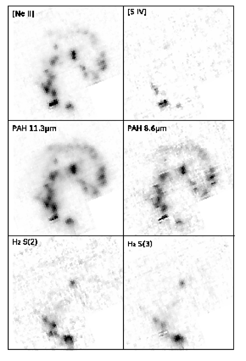
Figure 4.— IRS-SL spectral maps at the [Ne II] and [S IV] lines (top), the $11.3\mu$m and $8.6\mu$m PAH features (center), and the S(2) and S(3) rotational lines of H₂. The spectral continuum has been subtracted and the images shown represent the pure line intensities. The maps are shown in linear scaling. North is up, east is left. The images are approximately $135^{\prime\prime}$ (14.4 kpc) aside. For a discussion see Section 4.4

3.3. Fine-structure and Hydrogen Emission Lines

As can be seen in Fig. 3 the mid-IR wavelength range contains numerous strong fine-structure emission lines, most prominently from sulphur and neon. We measured the line fluxes from the ‘hires’ spectra using the Gaussian line fitting tool in SMART and a linear baseline fit. The results are listed in Table 5. The quoted uncertainties include the uncertainty in the absolute flux calibration, which we estimate to be of the order of 10%, and the fit errors provided by SMART. Both contributions have been added in quadrature.

Table 5Fine-structure line fluxes in units of $10^{-20}$W cm^-2

Line	[S IV]	[Ne II]	[Ne III]	[S III]	[Ar III]	[Fe III]	[O IV]	[Fe II]	[S III]	[Si II]
Wavelength	$10.51\mu$m	$12.81\mu$m	$15.56\mu$m	$18.71\mu$m	$21.83\mu$m	$22.93\mu$m	$25.89\mu$m	$25.99\mu$m	$33.48\mu$m	$34.82\mu$m
EP	34.97 eV	21.56 eV	40.96 eV	23.34 eV	27.63 eV	16.19 eV	54.93 eV	7.90 eV	23.34 eV	8.15 eV
nuc 4038	$\cdots$	$3.83\pm 0.40$	$0.29\pm 0.03$	$1.89\pm 0.20$	$\cdots$	$0.12\pm 0.02$	$0.12\pm 0.04$	$0.21\pm 0.03$	$2.75\pm 0.28$	$3.88\pm 0.39$
nuc 4039	$0.34\pm 0.04$	$2.41\pm 0.25$	$1.14\pm 0.12$	$1.91\pm 0.20$	$\cdots$	$0.11\pm 0.01$	$0.10\pm 0.69$	$0.23\pm 0.31$	$2.67\pm 0.27$	$3.25\pm 0.33$
peak 1	$1.25\pm 0.14$	$7.05\pm 0.77$	$4.44\pm 0.46$	$5.14\pm 0.52$	$0.05\pm 0.08$	$0.22\pm 0.04$	$0.14\pm 0.03$	$0.16\pm 0.04$	$7.64\pm 0.80$	$4.73\pm 0.51$
peak 2	$1.87\pm 0.19$	$6.64\pm 0.70$	$4.86\pm 0.49$	$6.22\pm 0.69$	$\cdots$	$0.30\pm 0.09$	$\cdots$	$0.26\pm 0.14$	$8.72\pm 0.93$	$5.19\pm 0.54$
peak 3	$0.78\pm 0.08$	$3.98\pm 0.41$	$2.48\pm 0.26$	$3.21\pm 0.32$	$\cdots$	$0.18\pm 0.02$	$0.13\pm 0.02$	$0.21\pm 0.03$	$6.09\pm 0.62$	$4.90\pm 0.50$
peak 4	$0.05\pm 0.01$	$2.11\pm 0.25$	$0.65\pm 0.07$	$1.37\pm 0.14$	$\cdots$	$0.06\pm 0.01$	$0.05\pm 0.01$	$0.10\pm 0.01$	$3.18\pm 0.32$	$3.18\pm 0.32$
peak 5	$0.39\pm 0.04$	$3.33\pm 0.34$	$2.31\pm 0.23$	$2.43\pm 0.25$	$0.05\pm 0.02$	$0.17\pm 0.02$	$0.17\pm 0.04$	$0.22\pm 0.02$	$5.14\pm 0.53$	$4.51\pm 0.46$
peak 6	$0.14\pm 0.02$	$2.47\pm 0.27$	$0.95\pm 0.10$	$1.71\pm 0.18$	$0.02\pm 0.00$	$0.07\pm 0.01$	$0.06\pm 0.01$	$0.10\pm 0.01$	$2.55\pm 0.26$	$3.23\pm 0.33$

Note. — The listed measurements have not been corrected for extinction. See comment to Table 3 for slit aperture sizes.

Our measurements of [Ne III] / [Ne II] are in the range of $0.08-0.75$, and hence lower than the [Ne III] / [Ne II] $\sim 0.8$ derived by Kunze et al. (1996) with ISO-SWS spectroscopy for the overlap region. However, our “line-luminosity weighted” average for the peaks 1, 2, 3, 5, and 6 together is $0.57^{+0.13}_{-0.11}$, still lower than but close to the ISO-SWS value of 0.8.

Fig. 3 also shows the lowest pure rotational transitions of molecular hydrogen, namely the 0-0 S(0) $28.21\mu$m, the 0-0 S(1) $17.03\mu$m, and the 0-0 S(2) $12.28\mu$m lines. In addition we find the atomic hydrogen lines of Humphreys-$\alpha$ H (7-6) $12.37\mu$m and the H I (8-7) $19.06\mu$m. The latter, however, has only been detected in the nucleus of NGC 4039. The line fluxes are listed in Table 6. The quoted uncertainties include the uncertainty in the absolute flux calibration, which we estimate to be in the order of 10% for the ‘hires’ spectra and 20% for the spectral maps, and the fit errors provided by SMART, again added in quadrature.

Table 6Line fluxes of molecular and atomic hydrogen in units of $10^{-20}$W cm^-2 observed in the IRS SL and SH modules.

Transition	H2S(3)	H2S(2)	H2S(2)	H2S(1)	H2S(0)	H (7-6)	H (8-7)
Wavelength	$9.67\mu$m	$12.28\mu$m	$12.28\mu$m	$17.03\mu$m	$28.22\mu$m	$12.37\mu$m	$19.06\mu$m
$E_{l}$	1015 K	510 K	510 K	170 K	0 K
nuc 4038	$0.71\pm 0.15$	$0.52\pm 0.11$	$0.64\pm 0.08$	$1.43\pm 0.15$	$0.72\pm 0.21$	$0.06\pm 0.01$	$\cdots$
nuc 4039	$3.76\pm 0.76$	$1.99\pm 0.42$	$1.11\pm 0.12$	$2.37\pm 0.24$	$0.43\pm 0.08$	$0.04\pm 0.05$	$0.05\pm 0.01$
peak 1	$\leq 0.50\tablenotemark{d}$	$0.39\pm 0.09$	$0.62\pm 0.08$	$1.64\pm 0.17$	$0.81\pm 0.09$	$0.15\pm 0.02$	$\cdots$
peak 2	$0.43\pm 0.11$	$0.45\pm 0.11$	$0.36\pm 0.06$	$1.23\pm 0.13$	$1.09\pm 0.24$	$0.11\pm 0.04$	$\cdots$
peak 3	$0.53\pm 0.12$	$0.45\pm 0.10$	$0.66\pm 0.07$	$1.77\pm 0.18$	$0.90\pm 0.10$	$0.11\pm 0.03$	$\cdots$
peak 4	$\cdots$	$\cdots$	$0.11\pm 0.03$	$0.19\pm 0.02$	$0.22\pm 0.05$	$0.06\pm 0.02$	$\cdots$
peak 5	$0.69\pm 0.14$	$0.67\pm 0.15$	$0.95\pm 0.11$	$2.38\pm 0.24$	$0.87\pm 0.10$	$0.11\pm 0.02$	$\cdots$
peak 6	$\cdots$	$\cdots$	$0.13\pm 0.03$	$0.24\pm 0.03$	$0.16\pm 0.02$	$0.05\pm 0.01$	$\cdots$

Note. — The listed measurements have not been corrected for extinction. See comment to Table 3 for the ‘hires’ slit sizes and Section 3.3 for the ‘lores’ apertures.

The line strength in the ‘lores’ spectra has been visualized and analyzed with CUBISM in the same way as the PAH features before. We concentrate the analysis on the strongest fine-structure and hydrogen lines within the range of the IRS-SL module to have similar spatial resolution for all maps (the slit width increases by a factor of two long-ward of $15\mu$m). Hence, we present the [S IV] map in Fig. 4 instead of [Ne III] which lies outside the range covered by the IRS-SL module.

We note that in ‘lores’ mode, the strong, adjacent emission features of [Ne II] at $12.81\mu$m and PAH at $12.7\mu$m cannot be fully spectrally resolved. From the ‘hires’ spectra we know that, on average, the luminosity in the PAH feature is about three times higher and thus a serious potential contaminant. A cross-contamination may lead to an over-estimation of the line flux, but also to an over-estimation of the continuum flux. For that reason we have excluded the $12.7\mu$m PAH feature from our analysis. A comparison of the [Ne II] line flux in the nucleus of NGC 4039 with the ‘hires’ spectrum, where the components are clearly resolved, indicates that the PAH contamination to the line flux is small ($\sim 20$%), and that the [Ne II] map is suitable for qualitative arguments.

The 0-0 S(1)$17.03\mu$m, the 0-0 S(2)$12.28\mu$m and the 0-0 S(3)$9.66\mu$m emission lines of molecular hydrogen were also detected in the ‘lores’ spectral maps. The S(2) and S(3) lines were both measured with the IRS-SL1 module, while the S(1) line was measured with the IRS-LL2 module at $\sim 2\times$ lower spatial resolution. Unlike the fixed ‘hires’ slit sizes and orientation, the apertures for the spectral maps, from which the ‘lores’ fluxes were extracted, were best matched to the size of the emitting region and vary from $5\times 4$ pixels ($960\times 768$ pc) to $10\times 11$ pixels ($1.92\times 2.11$ kpc) for the area around the nucleus of NGC 4039. The fluxes of the S(2) and S(3) lines have been added to Table 6. Fig. 4 shows the spectral maps at the [Ne II], [S IV], and the H₂ 0-0 S(2)$12.28\mu$m and S(3)$9.66\mu$m lines.

3.4. Deriving H₂ Temperatures and Masses

The H₂ lines serve as crucial diagnostics of the conditions of the ISM. The H₂ temperatures were calculated independently for the ‘lores’ and the ‘hires’ data as described in more detail in the Appendix and are listed in Table 9. Values range from approximately 270 K to 370 K.

However Table 9 does not list the uncertainties in the temperature and mass estimates because they are dominated by three components, which we discuss here. First are the errors in the line flux measurements, listed in Table 5. These are typically about 3%. Second, the different clusters suffer different amounts of extinction. Correcting for extinction has two effects: it increases the line fluxes and it changes the line ratios. For instance, a “typical” optical depth of $\tau_{9.7}=0.2$ would raise the temperature determined from the S(2) and S(3) lines by about 4% ($\sim 12$ K) since the S(3) is located in the center of the silicate band and suffers most from extinction. If we use the S(1) and S(2) lines instead, the temperatures rises only by 0.7% ($\sim 2$ K). The effect of extinction on the mass estimate is more complicated since it increases linearly with the corrected line flux but depends also on the temperature. For $\tau_{9.7}=0.2$ the H₂ mass increases by approximately 5%. Given the large uncertainties in the $A_{V}$ or $\tau_{9.7}$ for the clusters, as discussed in Section 3.5 and summarized in Table 7, we decided not to correct our tabulated estimates for extinction. Third, aperture effects play an important role. The ‘hires’ aperture is defined by the slit width and length and not matched to the size of the H₂ emitting region. For the ‘lores’ values the aperture was matched to the size of the region (Section 3.3). This systematic error is reflected in Table 9 by the difference between the corresponding mass estimates, and is the dominating uncertainty.

We have also calculated the H₂ masses following the procedure outlined in the Appendix. The derived masses are listed independently for the ‘lores’ and the ‘hires’ data in Table 9. Again, the two independent mass estimates using different lines and measurements from different instruments agree within $\sim 15$ % (except for peak 3), which provides confidence in the reliability of our measurements. A discussion of the derived H₂ masses is given in Section 4.11.

3.5. Extinction Estimates

The wavelength range covered by the IRS-SL and SH modules includes two important diagnostics to estimate the amount of dust: a broad Si=O stretching resonance, peaking at $9.7\mu$m, and an even broader O-Si-O bending mode resonance, peaking at $18.5\mu$m. We have estimated the extinction using the apparent optical depth in the $9.7\mu$m silicate feature. We assume extinction from a foreground screen, which is certainly an over-simplification. However, unlike for starburst galaxies as a whole, it is a reasonable approximation for the extinction toward individual, embedded SSCs, where the luminosity is provided by a central stellar cluster which is surrounded by dust and gas clouds and PDRs.

The depth of the $9.7\mu$m silicate feature was directly measured as the natural logarithm of the ratio of observed flux to the nominal mid-IR continuum at $9.7\mu$m. The latter can be best estimated (for PAH dominated spectra) by a power law fit anchored at $5.5\mu$m and $14.5\mu$m. The method is described and illustrated in Fig. 2 of Spoon et al. (2007). Our estimates of the optical depth are listed in the right column of Table 7.

Table 7Extinction estimates

Position	AV	AV	AV	$\tau_{9.7}$
peak 1	4.23	$6.2\pm 0.3$	$4.3\pm 0.3$	0.19
peak 2	0.18	$0.7\pm 0.1$	$1.4\pm 0.3$	0.13
peak 3	0.14	$4.8\pm 0.4$	$\cdots$	$\cdots$
peak 4	$\cdots$	$\cdots$	$0.6\pm 0.3$	$\cdots$
peak 5	11.81	$10.3\pm 0.5$	$\cdots$	1.03
peak 6	$\cdots$	$\cdots$	0.72	0.05

We disabled the PAHFIT default setting to automatically correct the measurements for extinction, and hence the values in Table 4 are the uncorrected, directly measured fluxes. This has been done for three reasons. First, PAHFIT has many free parameters, and given the limited spectral range of the IRS-SH module, which does not fully cover the $9.7\mu$m silicate band, extinction could be used as yet another free parameter to optimize the overall fit. Second, we do not, a priori, know whether a dust screen or mixed geometry provides a more realistic description. Third, the extinction at mid-IR wavelengths is generally rather low in these objects.

For a large sample of 172 near-IR sources in the Antennae, Brandl et al. (2005) found that the average extinction is about $A_{V}\sim 2$, while the reddest clusters may be attenuated by up to 10 magnitudes. From ISO-SWS spectroscopy of the hydrogen recombination lines Br_γ and Br_α in the overlap region Kunze et al. (1996) derived an extinction of $A_{V}\sim 70$ (mixed case) or $A_{V}\sim 15$ (screen extinction). The literature values are compared with our measurements in Table 7.

The conversion from $\tau_{9.7}$ to $A_{V}$ strongly depends on the assumed extinction law. Toward the Galactic Center there are various estimates: $A_{V}/\tau_{9.7}\sim 6.7$ (Moneti et al., 2001), $A_{V}/\tau_{9.7}\sim 7.8$ (Lutz, 1999), and $A_{V}/\tau_{9.7}\sim 9.0$ (Mathis, 1990). For the Solar neighbourhood Mathis (1990) derived $A_{V}/\tau_{9.7}\sim 18.5$, and Draine (1989) calculated $A_{V}/\tau_{9.7}\sim 18.1$. Given this broad range of conversion factors, we find that the estimates for $\tau_{9.7}$ from baseline fitting agree reasonably well with the other values listed in Table 7.

We note that the $\tau_{9.7}$ values indicate less extinction than derived from observations at shorter wavelengths, and the ratio of $A_{V}/\tau_{9.7}$ varies significantly from source to source. This may be caused by a dilution effect due to the large area covered by the IRS slits. An extended component of strong mid-infrared continuum emission will decrease the relative depth of the silicate absorption feature. This effect is likely most predominant for peak 1. Furthermore, optical methods mainly probe the absorption by graphite-based dust particles, while the mid-IR methods are mainly sensitive to distinct silicate absorption. In the diffuse ISM graphite and silicate-based dust are uniformly mixed and tightly correlated (Roche & Aitken, 1984). Recently, Chiar et al. (2007) found that in dense clouds with $A_{V}\geq 12$ the linear relation between optical and mid-IR estimates breaks down and $\tau_{9.7}$ underestimates the real amount of dust. However, most of our regions are below $A_{V}\sim 12$ and the discrepancy between the extinction values in Table 7 is primarily given by systematic uncertainties rather than ISM chemistry.

4. Results and Discussion

In this Section we discuss and interpret our observational findings from both the spectral maps and the spectra of the two nuclei and six infrared peaks. Our aim is to characterize the conditions under which SSCs form and evolve, their properties, and how their presence affects the surrounding interstellar medium. We start with a discussion of the individual regions, discuss qualitatively the ISM properties across the central region of the Antennae, investigate dust temperatures and radiation field, and derive cluster masses and star formation rates. We discuss the strength and variability of the PAH features and focus specifically on the strength of the H₂ emission and the temperature and excitation of the molecular hydrogen in the Antennae.

4.1. The Nuclei of NGC 4038 and NGC 4039

Based on sub-arcsecond near-IR spectroscopy from Keck, Gilbert et al. (2000) found that the spectrum of the nucleus of NGC 4039 is marked by a strong stellar continuum and bright, extended H₂ emission. These authors also found strong photospheric absorption of Mg I, Na I, and Ca I as well as from the CO $\Delta\nu=2$ band head absorption, indicating that the continuum is dominated by old giants and red super-giants. The Br_γ line, an indicator of recent massive star formation, was not detected. Mengel et al. (2001) found starburst activity a couple of arcseconds north of the nucleus of NGC 4038, consistent with an age of around 6 Myr. For the two nuclei Mengel et al. (2001) estimated an age of $65\pm 15$ Myr from CO absorption. It is clear that two galactic nuclei have lower star formation activity than the overlap region (Wang et al., 2004).

Chandra detected several X-ray sources near the radio positions of the nuclei of NGC 4038 and NGC 4039 (Zezas et al., 2002a). The X-ray sources identified with the nuclei are both luminous and spatially extended. The NGC 4038 nucleus spectrum is very soft and steep, and consistent with thermal emission by a supernova-driven super-wind, possibly with some contribution by X-ray binaries (Zezas et al., 2002a, b). The nucleus of NGC 4039 is more luminous in X-rays, but its spectrum also suggests a combination of X-ray binaries and compact supernova remnants (Zezas et al., 2002a, b). The NGC 4039 nucleus also has a very steep radio spectrum (Neff & Ulvestad, 2000) suggesting that its radio emission is non-thermal, arising from supernova remnants. These observations are consistent with the intermediate starburst age of about 65 Myr estimated by Mengel et al. (2001). The supernovae may be responsible for heating the ISM in the nuclear region to the observed X-ray temperatures, and the X-ray emission, and shocks arising from the supernovae may also be responsible for the high-excitation line emission. At any rate, neither X-ray nor radio observations have provided strong evidence for activity due to black hole accretion in either nucleus.

The IRS spectra of the two nuclei are quite similar in terms of their PAH strength and silicate absorption (Fig. 3). However they differ significantly regarding their mid-IR fluxes, 20-30$\mu$m slopes, and fine-structure lines. As mentioned in Section 2.1 the observed position of the nucleus of NGC 4038 is slightly offset to the north of the radio nucleus, and the wide IRS-SH slit includes the nearby star forming region as well. Hence, the detected mid-IR emission is likely affected by the starburst activity to the north of the nucleus of NGC 4038. The nucleus and the nearby starburst region can be seen in most of the spectral maps in Fig. 4 as an extended structure with two separate components. The strong high excitation lines in the NGC 4039 nucleus pose somewhat more of a puzzle. The [Ne III]/ [Ne II] ratio is almost six times higher in NGC 4039, and the [S IV] line is also very strong in NGC 4039, while it has not been detected in NGC 4038.

In the mid-IR AGN activity can usually be traced by the high excitation [O IV] and [Ne V] emission lines (Spinoglio & Malkan, 1992; Sturm et al., 2002; Weedman et al., 2005). However, the best indicators, the [Ne V] lines at 14.3 and $24.3\mu$m, were not detected in either nucleus. The [O IV] line is not produced in measurable quantities in Hii regions but can be excited by hot Wolf-Rayet stars, shocks, and AGN. In a study of starburst galaxies with ISO Lutz et al. (1998) defined the ratio [O IV] / ([Ne II]$+0.4\times$[Ne III]), and found values ranging between 0.006 (M82) and 0.062 (II Zw 40) with a mean of 0.022. As can be seen from Table 5 our ratios for the peaks 1, 3, 4, 5 and 6 are 0.016, 0.026, 0.021, 0.040 and 0.021, respectively – all in excellent agreement with the mean starburst value of Lutz et al. (1998). For the two nuclei of NGC 4038 and NGC 4039 we find ratios of 0.030 and 0.035, respectively. Both ratios are also well within in the range covered by “pure” starburst systems and provide no evidence for AGN activity. This finding is further supported by the large equivalent widths of the PAH features (Tab. 4), which would not be expected in the surroundings of an accreting black hole (e.g., Weedman et al., 2005).

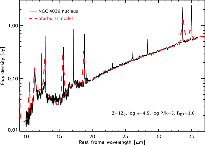
Figure 5.— IRS spectrum of the NGC 4039 nucleus (thin curve) with the best fitting starburst SED model template from Groves et al. (2008) (thick dashed curve).

Besides the high excitation lines, arguably the best mid-IR diagnostic for the presence of an AGN is the spectral continuum. Hot dust around an AGN will significantly flatten the continuum slope (see e.g., Fig. 8 in Brandl et al. (2006)). In Fig. 5 we compare the spectrum of the nucleus of NGC 4039 to a starburst model of Groves et al. (2008) chosen to best match the dust continuum and the PAH features. The determined parameters of the fit indicate that the nuclear abundances are similar to Solar ($\sim 1$ Z_⊙), with the star formation occurring in somewhat distributed manner ($\log{\cal C}=4.5$) in regions with standard ISM pressures ($\sim\rm{P}_{0}/k=10^{5}$ K cm^-3), but still reasonably embedded within their molecular gas birth clouds ($\sim f_{\rm PDR}\sim 1.0$). (For a full description of the parameters see Groves et al. (2008)). The good match between the observed continuum and a “pure” starburst model shows that the spectrum of the nucleus of NGC 4039 is fully consistent with emission from dust that is heated by star formation only.

4.2. The Properties of Individual SSCs

Four of our six infrared peaks, namely peaks 1, 2, 3, and 5, are located in the overlap region (Fig. 1), which is the region of the most intense star formation in the Antennae (Mirabel et al., 1998; Vigroux et al., 1996); peaks 4 and 6 are located outside the overlap region. In this subsection we summarize briefly some of their properties based on information from the literature. Some cluster masses are discussed in Section 4.6.

Peak 1 coincides with a clump of molecular gas as traced by CO (peak CO_S and SGMC 4–5, Stanford et al., 1990; Wilson et al., 2000, 2003). It is also the brightest source at centimeter wavelengths, and the spectral index of the radio emission indicates that the spectral energy distribution is dominated by the thermal radiation from Hii regions (Hummel & van der Hulst, 1986) with an equivalent of $\sim$ 5000 O5 stars (Neff & Ulvestad, 2000). However, the optical counterpart to this source corresponds to a very inconspicuous, faint, red source in the HST images (Whitmore & Schweizer, 1995, source 80) obscured by large amounts of gas and dust. Based on sub-arcsecond near- and mid-IR spectroscopic data, both Gilbert et al. (2000) and Snijders et al. (2007) find an ionized gas density of $10^{4}$ cm^-3.

Peak 2 is the mid-IR counterpart to a bright and blue complex of clusters, which contains eight optical sources within a region of 1$\farcs$5 (Whitmore & Schweizer, 1995), corresponding to 160 pc in projection at our adopted distance. Peak 2 also corresponds to the second brightest radio source in the Antennae. Like peak 1 it has a shallow spectral slope, typical for the emission from Hii regions (Hummel & van der Hulst, 1986; Neff & Ulvestad, 2000) with an equivalent of $\sim$ 3000 O5 stars. The density of the ionized gas has been estimated to be $\sim 10^{4}$ cm^-3 (Snijders et al., 2007).

Peak 3 corresponds to the center of the largest concentration of molecular gas in the overlap region. The coincident sources CO_F and part of SGMC 1 (Stanford et al., 1990; Wilson et al., 2000, 2003) contain a total molecular gas mass over $6\cdot 10^{8}$  M_⊙. The slope of the corresponding bright, compact radio source (Neff & Ulvestad, 2000) is steep, arguing for a somewhat older cluster with its radio emission being dominated by supernova remnants.

Peak 4 is located to the far west of the nucleus of NGC 4038. The radio observations show a moderately bright, compact source with a steep spectral slope, indicative of an evolved stellar population (Hummel & van der Hulst, 1986; Neff & Ulvestad, 2000).

Peak 5 is located in the overlap region, approximately 1.6 kpc to the north-west of peak 1, and is the brightest sub-millimeter peak. It coincides with the sources CO_W and part of SGMC 1 (Stanford et al., 1990; Wilson et al., 2000, 2003), which are huge concentrations of approximately $3.9\cdot 10^{8}$ M_⊙ of molecular gas. With an A${}_{V}\sim 11.81$ it is one of the most heavily embedded clusters in the Antennae (Mengel et al., 2005). Its optical counterpart is identified as the red source 115 in Whitmore & Schweizer (1995). Peak 5 also coincides with a bright, compact radio source (Neff & Ulvestad, 2000). The spectral index suggests that the dominant radio emitters are supernova remnants.

Peak 6, finally, is a mid-IR source located in a region of more extended, fuzzy IR emission, to the east of the nucleus of NGC 4038. The spectral slope of the radio emission is at the division point between the radiation field of Hii regions and supernova remnants.

4.3. Cluster Ages

The age estimates depend significantly on the method being used, and show significant scatter. The literature values on cluster ages of all our clusters are summarized in Table 8. The various age diagnostics indicate that the luminous IR sources in the northern part of the overlap region are somewhat older than the ones in the more active, southern overlap region.

Table 8Cluster Ages from the Literature

	Age	Age	Age	Age	Age
Position	[Myr]	[Myr]	[Myr]	[Myr]	[Myr]
peak 1	2.0	$2.3-4.0$	3.5	$\leq 2.5$	2.5
peak 2	3.8	$2.3-4.0$	$\cdots$	$\leq 3$	3.0
peak 3	2.0	$3.2-4.9$	3.9	$\leq 3$	3.0
peak 4	7.0	$\geq 6$	$\cdots$	$\cdots$	7.0
peak 5	$\cdots$	$3.7-5.1$	5.7	$3-5$	4.5
peak 6	8.4	$4.3-5.7$	$\cdots$	$\cdots$	6.0

In Fig. 6 we compare the average cluster ages from the literature (Tab. 8) to the radiation hardness measured by the [Ne III] / [Ne II] line ratio. There is a clear trend of older clusters displaying a softer radiation field due to the disappearance of the early-type O and Wolf-Rayet stars after about 5 Myr. While this result may not come as a surprise it is reassuring that completely independent methods are consistent.

Figure 6.— The hardness of the radiation field (as measured by the line flux ratio of [Ne III] / [Ne II]) versus the average age of the SSCs from Table 8. The horizontal dotted lines indicate the age ranges covered by the various estimates.

We note that starburst activity exists to both east (including peak 6) and west (including peak 4) of the nucleus of NGC 4038 at almost the same level, in terms of the [Ne II] and PAH intensity. In fact, peaks 4 and 6 have almost identical mid-IR spectra (Fig. 3), yet are separated by more than 6.6 kpc in projection. With a velocity dispersion of $\sim 10$ km s^-1 (Whitmore et al., 2005) the dynamical time to connect the two points would be 647 Myr, about two orders of magnitude longer than the cluster ages. This suggests that the dominant mode of triggering the formation of SSCs does not propagate hydrodynamically but is governed by local processes.

4.4. Physical Conditions across the Antennae

In this subsection we discuss the spatial variations in the ISM as revealed by the spectral maps shown in Fig. 4. These maps provide a more global picture of the physical conditions across the central region of the Antennae galaxies. Unfortunately, the [Ne III] line, which we utilize heavily in Section 4.5, is not covered by the IRS-SL module and would have to be observed through the much wider IRS-LL slit. However, given that the excitation potential of [Ne III] is reasonably close to that of [S IV] (see Table 5), we substitute the [S IV] line as a tracer of the harder radiation.

Fig. 4 (top) compares the maps of [Ne II] with [S IV]. It takes only 21.6 eV to excite [Ne II], and the emission traces primarily the regions where star formation occurred in the past $\sim 10$ Myr. (As a rule of thumb we assume that [Ne II] is primarily associated with stars younger than $\sim 10$ Myr, while [S IV] traces stars younger than $\sim 4-6$ Myr in a starburst). The [S IV] emission originates predominantly from two clusters peaks 1 and 2 in the overlap region, with peak 2 being even brighter in [S IV] than peak 1 (Fig. 4). Although this has already been indicated by the spectra in Fig. 3, and qualitatively known since ISO (Mirabel et al., 1998), it is once again remarkable how the bulk of the current massive star formation in an interacting system, which extends over tens of kilo-parsecs, is confined to just two compact regions. We also detect some [S IV] emission from the nucleus of NGC4039, but none from 4038 (Section 4.1). The [Ne II] map is also dominated by the two clusters peak 1 and 2, although to a much lesser degree than the [S IV] map, and also shows emission from the nucleus of NGC 4038. Noticeable [Ne II] emission is also detected to the west of the nucleus of NGC 4038, where numerous older SSCs reside (Mengel et al., 2005).

Overall, the PAH maps in Fig. 4 (center row) resemble the [Ne II] map, but show noticeably more diffuse emission. In “normal” galaxies a predominant fraction of the total PAH emission arises from the diffuse ISM, heated only by the interstellar radiation field, with a only a low fraction rising from PDRs (Draine et al., 2007). However in starbursting galaxies like the Antennae the situation is reversed, with the major part of the total emission coming from the regions of recent star-formation. Here the PAH maps trace primarily the PDRs and hence the environment of OB clusters. However, the fact that the [Ne II] and PAH map resemble each other qualitatively implies that we do not resolve the Hii region/PDR interfaces at the spatial resolution of the IRS-SL spectral map, which is between 200 – 380 pc, depending on wavelength and orientation.

The most obvious difference between the [Ne II] and the PAH maps is the strength of peaks 1 and 2 relative to the nucleus of NGC 4038. The latter is the dominant source of PAH emission, while the embedded SSCs play only a minor role. Within the uncertainties, which are dominated by the lower signal-to-noise in the $6.2\mu$m map, we find no significant differences between the $11.3\mu$m and the $6.2\mu$m PAH maps. (We note that the PSF in the former is also 1.8 times larger). The similarity between the two PAH maps agrees with our study of the PAH spectrum in Section 4.8.

The bottom row in Fig. 4 shows the spectral maps in the H₂ S(2) and S(3) lines. Both maps are very similar. We find that approximately 45% of the total H₂ S(3) emission comes from a slightly extended region around the southern nucleus, NGC 4039. The nucleus of NGC 4038 does show some H₂ emission, but very little compared to NGC 4039. The emission peaks of the clusters in the overlap region are more compact and also weaker. Most interesting here is the small spatial offset of about two pixels, corresponding to approximately 380 pc, that exists between the peaks of H₂ emission and the spectral continuum, for both peak 5 and the nucleus of NGC 4039. The H₂ S(2) emission peaks to the south in both objects and appears also, at least near the nucleus on NGC 4039, more extended. Since the offsets are with respect to the continuum emission, which was simultaneously observed with the line emission, they cannot be due to spacecraft pointing errors or other observational effects. Rather they must arise from a physical displacement between the massive SSCs and the source of H₂ emission.

Finally, we compared the $8.6\mu$m PAH map with the IRAC $8\mu$m image of Wang et al. (2004). Despite the slightly better spatial resolution of the IRAC image both maps look very similar with one exception: the emission from peak 1 is noticeably brighter in the IRAC image than in the $8.6\mu$m PAH map. The spectra in Fig. 3 and the values in Table 4 show that the PAH equivalent widths of peaks 1 and 2 are significantly below those of the other clusters. Although the IRAC $8\mu$m band is generally dominated by PAH emission, a proper continuum subtraction is obviously important for quantitative results.

4.5. Dust Temperature and Radiation Field

The mid-infrared continuum $\geq 20\mu$m is produced by the thermal emission from dust heated by the stellar clusters. The slope of the continuum reflects the temperature distribution of the dust. The presence of a hot dust component (100 K $\leq T\leq$ 250 K) flattens the continuum slope in the wavelength range of $15-35\mu$m, while a cold dust component ($T\leq 50$ K) steepens the slope. The continuum fluxes at $15\mu$m and $30\mu$m and their ratios are listed in Table 3. Peaks 1 and 2 have the shallowest slopes, indicating the highest dust temperatures, while peaks 3 and 5 show the steepest continua, evidence for a dominating dust component at lower temperature. The difference is also illustrated in Fig. 7 for the most extreme cases of peaks 1 and 5, in comparison to the average starburst galaxy spectrum from Brandl et al. (2006). The slope of the starburst template lies between the two Antennae clusters.

Figure 7.— Comparison of the $14-37\mu$m continuum slopes for three selected objects: peaks 1 and 5 with the most shallow and steep slopes in our sample of Antennae clusters, and the average starburst template spectrum from Brandl et al. (2006). The spectra are plotted in units of $\nu F_{\nu}$ to enhance the differences, and have been normalized to unity at $15\mu$m.

Generally, the dust temperature depends on a complex relation between ISM density, grain size distribution, stellar properties, strength of the radiation field, and the local geometry of cluster, Hii region, PDR, and surrounding ISM. We have investigated possible correlations of the dust temperature with cluster properties from the literature and our measurements, such as cluster age (Table 8), mid-IR luminosities (Table 3), extinction (Table 7), PAH strength (Table 4), hardness of the radiation field (Table 5) or star formation rate (Table 9). However, no statistically convincing correlation between these quantities has been be found.

4.6. Cluster Luminosities and Star Formation Rates

The mid-IR continuum fluxes can be used to estimate the total infrared luminosity of starburst systems (in which $L_{\rm IR}\approx L_{bol}$). In their Section 4.2 Brandl et al. (2006) discuss a method based on the $15\mu$m and $30\mu$m continuum fluxes. Adopting their empirical relation and a distance of 22 Mpc (Schweizer et al., 2008) we get $L_{\rm IR}=2.067\cdot F_{15}+5.324\cdot F_{30}$ in units of $10^{9}$ L_⊙. We note that this empirical relation was derived for global starbursts, where the temperature components may different from the one in and around more compact SSCs. However, the good agreement in Fig. 7 between the slopes of the various systems indicates that the estimate works reasonably well.

In Table 9 we list the mid-IR derived cluster luminosities. The infrared luminosities of the eight compact regions already add up to $L_{\rm IR}=3.82\cdot 10^{10}$ L_⊙. The total infrared luminosity of the Antennae, measured from the four IRAS bands at our distance, is $L_{\rm IR}=7.2\cdot 10^{10}$ L_⊙(Sanders et al., 2003). Hence, the eight individual regions studied here account for slightly more than half of the total luminosity of the system.

Table 9Derived Cluster Properties

	$L_{\rm IR}$	SFR	T(H2)	T(H2)	M(H2)	M(H2)
Position	[$10^{9}$ L⊙]	[ M⊙/yr]	[K]	[K]	[$10^{6}$ M⊙]	[$10^{6}$ M⊙]
nuc 4038	3.67	0.63	329	327	1.78	2.24
nuc 4039	1.86	0.33	378	334	3.97	3.56
peak 1	11.41	1.97	$\cdots$	302	$\cdots$	3.09
peak 2	10.40	1.81	288	267	2.82	3.20
peak 3	4.35	0.74	311	300	1.97	3.39
peak 4	1.29	0.22	$\cdots$	374	$\cdots$	0.22
peak 5	3.86	0.66	296	309	3.67	4.24
peak 6	1.31	0.22	$\cdots$	360	$\cdots$	0.30

Note. — For uncertainties in the H₂ mass and temperature estimates see Section 3.4. The S(3)flux from peak 1 was well detected but is uncertain due to a data artifact.

Kennicutt (1998) has shown that the $8-1000\mu$m infrared luminosity $L_{\rm IR}$ of starbursts is a good measure of the SFR as given by

$$\mbox{SFR}\ [M_{\odot}\mbox{yr}^{-1}]=4.5\cdot 10^{-44}L_{\rm IR}\ [\mbox{erg\ s}^{-1}].$$

We note that the SFR conversion given by Kennicutt (1998) strictly applies only to dusty starbursts in the continuous star formation approximation, with ages of order $10-100$ Myr. Our clusters are significantly younger than that, so in the continuous star formation approximation (which is a reasonable one, given the more or less continuous range of cluster ages, as seen in Fig. 6) the IR luminosity per unit mass of stars formed will be somewhat lower. In other words, for regions younger than 10 Myr the Kennicutt (1998) relation will systematically overestimate the SFRs.

Our estimated SFRs for the individual clusters are listed in Table 9. Co-adding the eight regions we get a total $\mbox{SFR}\approx 6.6$ M_⊙ yr^-1. Given the compact sizes of the regions our results agree with Wang et al. (2004), who derived from Spitzer-IRAC $3-8\mu$m observations that the rates of star formation in the active regions are as high as those seen in starburst and some ultraluminous infrared galaxies on a “per unit mass”basis.

As a cross-check we compare our SFRs to an independent estimate by dividing the stellar masses of the clusters from the literature by their ages. For peak 1 Mengel et al. (2001) determined $3\cdot 10^{6}$ M_⊙ and Snijders & van der Werf (2007) found $1.1-1.2\cdot 10^{6}$ M_⊙. For peak 2 Mengel et al. (2001) found $1.6\cdot 10^{6}$ M_⊙ and Snijders & van der Werf (2007) measured $1.2-1.7\cdot 10^{6}$ M_⊙. For average cluster masses of $2\cdot 10^{6}$ M_⊙ and $1.5\cdot 10^{6}$ M_⊙ for peaks 1 and 2, and ages of 2.5 and 3.0 Myr (Table 8) we estimate (continuous) star formation rates of 0.8 and 0.5 M_⊙ yr^-1, respectively. These rates are roughly a factor of three below the SFRs derived from the mid-IR fluxes. However, we emphasize the substantial systematic uncertainties in these estimates. Snijders & van der Werf (2007) assumed a Salpeter IMF from $0.1-100$ M_⊙, while Mengel et al. (2001) assume a lower mass cutoff of 1 M_⊙, corresponding to a 2.6 times smaller cluster mass. Using the same IMF would lead to mass differences between those studies of factors of 6.5 and 2.9 for peaks 1 and 2, respectively.

The sum of the SFRs around the two nuclei and the six infrared-brightest regions ($4.8\cdot 10^{6}$ pc² in total) as listed in table 9 is 6.6 M_⊙ yr^-1. As stated above, our method will likely provide an overestimate of the true SFR. On the other hand, star formation will also occur outside our regions at a reduced rate. Hence, we consider our estimate of 6.6 M_⊙ yr^-1, within 50%, as representative for the SFR in the Antennae galaxies.

We also note that Zhang, Fall & Whitmore (2001) determined a rather large SFR of 26 M_⊙ yr^-1 for a distance of 22 Mpc. Using the Kennicutt (1998) relation between SFR and $L_{\rm IR}$ this would correspond to a more than two times higher total infrared luminosity than the one derived from the IRAS bands (Sanders et al., 2003), and would move the Antennae to the class of LIRGs. Hence, we consider the SFR derived by Zhang, Fall & Whitmore (2001) an overestimate.

Recently, Smith et al. (2007c) investigated Spitzer photometry of a sample of 35 tidally distorted pre-merger interacting galaxy pairs selected from the Arp atlas. These authors found a very modest enhancement of the SFRs at early stages of $\sim 1$ M_⊙ yr^-1 on average. Although the Antennae is still in an early stage of interaction (Mihos & Hernquist, 1996) it shows an enhanced SFR, well above the sum of typical star formation in two normal spiral galaxies. With its ample amount of molecular gas (Gao et al., 2001) the system is likely to become an even more spectacular starburst after one or two orbits.

4.7. PAH Strength and Aperture Effects

PAHs are considered the most efficient species for stochastic, photoelectric heating by UV photons in PDRs (Bakes & Tielens, 1994). They are usually a good tracer of starburst activity in a statistical sense (e.g., Brandl et al., 2006, and references therein). However, numerous studies over the past two decades (e.g. Geballe et al., 1989; Cesarsky et al., 1996; Tran, 1998) have shown that intense UV fields can lead to the gradual destruction of PAH molecules. A clear anti-correlation between the $11.3\mu$m PAH strength and the radiation field across the central region of NGC 5253 was recently observed by Beirão et al. (2006). We investigate this effect for the Antennae in two different ways: via a pixel-by-pixel analysis within the spectral map and for the eight ‘hires’ spectra.

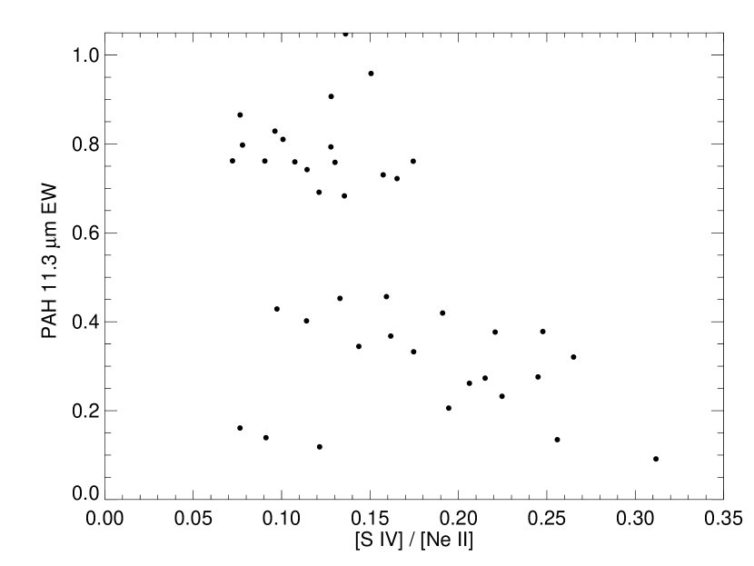
Figure 8.— The relative strength of the $11.3\mu$m PAH feature (a normalized “line”-to-continuum ratio) versus the hardness of the radiation field as expressed by the line ratio of [S IV] / [Ne II]. Each data point corresponds to one pixel in the spectral map. Only those 42 pixels with a signal of greater than four standard deviations in the S IV map have been included.

The former is shown in Fig. 8 where the $11.3\mu$m PAH-to-continuum ratio is plotted versus the hardness of the radiation field as expressed by the line ratio of [S IV] / [Ne II]. Each data point in Fig. 8 corresponds to a spatial pixel in our spectral map for which the signal-to-noise at [S IV] is greater than four standard deviations. (See section 3.3 concerning the contamination of [Ne II] by the $12.7\mu$m PAH emission in ‘lores’ mode). Fig. 8 reveals a trend that regions with harder radiation fields show relatively weaker PAH emission.

We note that the strength of the [S IV] relative to the [Ne II] line does not only depend on the hardness of the radiation field, but is sensitive to the gas density as well. Given the critical densities of $3.7\cdot 10^{4}$ cm^-3 and $6.1\cdot 10^{5}$ cm^-3 for [S IV] and [Ne II], respectively (Tielens, 2005, and references therein), it is expected that densities above $10^{4}$ cm^-3 will decrease the [S IV] / [Ne II] ratio. Model calculations with CLOUDY show that an increase in density from $10^{4}$ to $10^{5}$ cm^-3 can cause a decrease in [S IV] / [Ne II] by a factor of three, contributing significantly to the scatter in Fig. 8.

To quantify the strength of the radiation field we use the line fluxes of [Ne II] and [Ne III] and the parametrization of Beirão et al. (2006):

$$\left(F_{\rm[Ne\,II]12.8\mu m}\,+\,F_{\rm[Ne\,III]15.6\mu m}\right)\times\frac{F_{\rm[Ne\,III]15.6\mu m}}{F_{\rm[Ne\,II]12.8\mu m}}.$$

The first factor, $F_{\rm[Ne\,II]12.8\mu m}\,+\,F_{\rm[Ne\,III]15.6\mu m}$, is a measure of the intensity of the field, assuming that all Neon exists in one of the two ionization states. The second factor, $\frac{F_{\rm[Ne\,III]15.6\mu m}}{F_{\rm[Ne\,II]12.8\mu m}}$, is a measure of the radiation field hardness. We define the product of intensity and hardness as the “strength” of the radiation field.

Figure 9.— The relative strength of all PAH features within the $10-20\mu$m range versus the strength of the radiation field.

In Fig. 9 we plot the strength of the PAH features, measured from the ‘hires’ spectra, against the strength of the radiation field. On the ordinate we plot the average PAH strength calculated by co-adding all the PAH fluxes listed in Table 4 and normalizing them to the $15\mu$m continuum flux (Table 3). There is a clear linear anti-correlation between the strength of the PAH emission and the radiation field. The only outlier is the inactive nucleus of NGC 4038.

Both rather independent methods and data sets provide statistical evidence that the strength and hardness of the radiation field affect the PAH emission. However, we cannot be certain that this effect is actually due to a destruction of PAH molecules in stronger radiation fields. The sources with the strongest PAH “equivalent width” are peaks 4 and 6. Both are located in less dense regions. These clusters are also slightly older and have had more time to shape the surrounding ISM via stellar winds and SNe. If the size of the emitting region is radiation-bounded these regions may just have “grown” more complex Hii region/PDR interfaces from where the PAH emission originates. In other words, the PDR surface area is higher relative to the thermal emission from dust in the denser regions, which produces the underlying continuum.

Unfortunately, with the wide IRS-SH slit width, corresponding to 500 pc, we cannot resolve the Hii region/PDR interfaces. However, some of the clusters were recently observed by Snijders et al. (2006) with VISIR on ESO’s VLT using a sub-arcsecond slit corresponding to only 75 pc at our distance of 22 Mpc. Comparing our IRS-SH spectra of peaks 1 and 2 to their VLT-VISIR spectra, Snijders et al. (2006) found that, while the continuum fluxes observed with both instruments are quite similar, the wider IRS slit detects much stronger PAH emission. The individual clusters are by far the most luminous sources on projected scales of a few hundred parsecs, and we may observe the profound effect of the OB clusters on their surrounding ISM. However, Snijders et al. (2006) concluded that a large fraction of the PAH emission cannot be directly associated with the SSCs but originates from an extended region around the cluster. In fact, if the space density of young clusters near peaks 1 and 2 is significantly higher than elsewhere it could be that the extended PAH emission, which is only picked up by the IRS, is unrelated to the main clusters and externally excited by smaller clusters in the immediate vicinity of peaks 1 and 2. At this point we cannot distinguish between a giant Hii region of a hundred or more parsecs in diameter and a locally enhanced density of OB clusters. A significant improvement will have to wait for the next generation of extremely large telescopes (ELTs).

4.8. (In-)Variability of the PAH Spectrum

We have also investigated possible variations of the PAH spectrum. While – to first order – the strengths of the PAH features are observed to scale with each other (e.g., Smith et al., 2007b, Fig. 6), the PAH spectrum is expected to depend on the grain size distribution (Draine & Li, 2001, 2007): smaller PAHs are more likely to emit at shorter wavelengths while larger PAHs are more likely to produce stronger features at longer wavelengths. We utilize the longest baseline provided by the ‘hires’ spectra between strong PAH features and selected the $11.3\mu$m feature and the $17\mu$m PAH complex. We find an average $17\mu$m / $11.3\mu$m PAH ratio of 0.4 (Table 4) with some scatter but no significant correlation with any other observed quantity. From the SINGS sample of galaxies Smith et al. (2007b) have found that the $17\mu$m / $11.3\mu$m PAH ratio increases with increasing metallicity. Assuming solar abundance for the Antennae (Bastian et al., 2006) our PAH ratio of 0.4 is consistent with the measurements of Smith et al. (2007b, Fig. 16) although somewhat on the low side.

Another cause of potential variations of the PAH spectrum may be ionization effects. Several authors (e.g., Verstraete et al., 1996; Vermeij et al., 2002; Förster Schreiber et al., 2003) have reported on variations in the PAH spectrum, namely that the C–C stretching modes at $6.2\mu$m and $7.7\mu$m are stronger in ionized PAHs, relative to the bending mode at $11.3\mu$m – by factors of up to two. Here we use the ratio of the $8.6\mu$m C–H in-plane bending mode to the $11.3\mu$m C–H out-of-plane bending mode, which is also sensitive to the charge state of the PAH molecule (Hudgins & Allamandola, 1995; Joblin et al., 1996). We have chosen these two for a direct comparison because of their proximity in wavelength (same beam size), similar susceptibility to dust extinction, and because both are observed through the same IRS (sub-)slit. Smith et al. (2007b) investigated the $7.7\mu$m / $11.3\mu$m PAH ratio as a function of the hardness of the radiation field and found no significant correlation for the Hii-nuclei in the SINGS galaxies sample (their Fig. 14).

Fig. 4 already indicates that, to first order, both PAH maps trace each other quite well. Thus we have computed the ratio on a pixel-by-pixel basis between the two $8.6\mu$m / $11.3\mu$m PAH maps. The map is shown in Fig. 10 at two times lower resolution to reduce the noise. Regions with relatively stronger $8.6\mu$m emission appear brighter, regions with relatively stronger $11.3\mu$m emission appear darker in this ratio map. While the emission from the nucleus of NGC 4038 appears in average “gray” the peaks 3, 5, and 6 appear darker and have values about 20% above the mean. On the other hand, peaks 1 and 2, the most massive clusters, appear brighter by about the same amount. These variations are not correlated with extinction effects, which would affect the values in the opposite direction. However, we emphasize that the noise, in particular in the $8.6\mu$m map (Fig. 4), is quite significant. Although these variations may provide weak evidence for changes in the PAH spectrum on cluster scales, a conclusive analysis requires better resolution and lower noise.

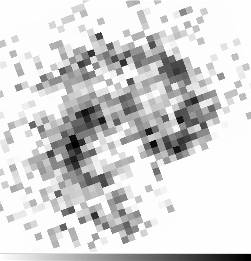
Figure 10.— IRS spectral map of the $8.6\mu$m / $11.3\mu$m PAH ratio. The median ratio has been normalized to unity, which is colored in mean gray, and the range extends over a factor of two to both sides. Brighter regions represent relatively stronger $8.6\mu$m emission, darker regions weaker $8.6\mu$m emission. Field size and orientation are as in Fig. 4 but the resolution has been reduced by rebinning by a factor of two to suppress the noise.

4.9. Strength of the H₂ Emission

Molecular hydrogen is the most abundant molecule in the Universe. It plays a central role in star formation, not only as the major ingredient to build up a star but also as the coolant to permit an isothermal collapse of the gas cloud. The density and temperature of the H₂ molecule are of utmost importance for the processes in starbursts. However, the H₂ molecule is symmetric, has no dipole moment, and the mid-IR lines originate from quadrupolar rotational transitions. Consequently, the lines are intrinsically weak and usually hard to detect. Since the first study of the S(2) line in Orion by Beck et al. (1979) and the detection of the S(0) line in NGC 6946 by Valentijn et al. (1996), the mid-IR rotational lines in starbursts have been studied by numerous groups. Most relevant in our context are the ISO-SWS studies by Rigopoulou et al. (2002), the review by Habart et al. (2005), and the Spitzer-IRS studies of ULIRGs by Higdon et al. (2006), and SINGS galaxies by Roussel et al. (2007).

The H₂ lines in the Antennae are amongst the strongest detected lines (Fig. 3). We have calculated the total, spatially integrated H₂ S(2) and S(3) line fluxes by summing up all pixels where the signal-to-noise was greater than three standard deviations in the spectral maps and compared them to the sum of the regions listed in Table 6. In the S(3) line essentially all of the measured flux of $6.1\cdot 10^{-20}$ W cm^-2 originates from our designated regions. The emission in the S(2) line is slightly more extended and the spatially integrated measure picks up 27% more flux than listed in Table 9. We conclude that most of the total amount of warm H₂ over the central Antennae system is concentrated around our eight sources.

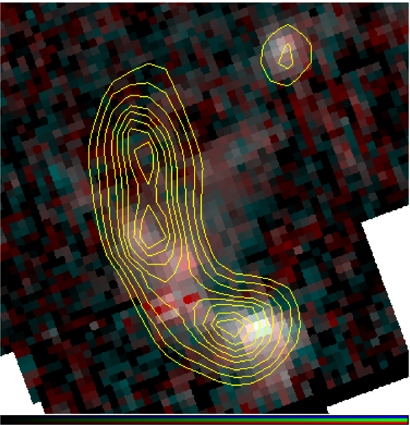
Figure 11.— False-color IRS spectral map of the H₂ S(3) line in the green and blue channel, and the S(2) line in the red channel in square-root scaling. Bluer colors mean warmer H₂. North is up. The two nuclei and the emission from the clusters in the overlap region are clearly visible. The yellow contour lines indicate the ISOCAM-CVF measurements of the H₂ S(3) line by Haas et al. (2005); the levels are at 39%, 49%, 58%, 68%, 78%, 84%, 90%, and 96% of the maximum intensity (see Fig. 2 in Haas et al. (2005)).

Fig. 11 shows a false-color image of the IRS maps with the H₂ S(3) and S(2) lines in blue/green and red. Both nuclei and the emission from the active overlap region are clearly visible. The map shows that the largest portion (approximately 45%) of the total H₂ S(3) emission comes from a region around the southern nucleus. The strongest H₂ emitter in the active overlap region is peak 5.

We note that our integrated H₂ S(3) line flux of $6.1\cdot 10^{-20}$ W cm^-2 is about five times below the S(3) line flux of $3.3\cdot 10^{-19}$ W cm^-2 which Haas et al. (2005) have found. In Fig. 11 we overlaid the contours of their ISO H₂ S(3) intensity map for comparison. While our peak 5 is close to their southern peak of the contour map, the northern peak of the contour map has no luminous counterpart in our map. Our closest peak is peak 6, which contains more than an order of magnitude less H₂ mass than peak 5. We have also checked the IRS-LL map, which includes the H₂S(1) emission line, albeit at two times lower spatial resolution, and confirmed the strong drop in H₂ emission northward of peak 3. Altogether, we cannot confirm the claim by Haas et al. (2005) of strong H₂ emission from a region extending farther to the north of the overlap region, well beyond the most active area. These differences in distribution and total line fluxes have significant impact on the derived H₂ masses for the Antennae system.

At the distance of 22 Mpc, our S(3) line flux corresponds to a line luminosity of $9.2\cdot 10^{6}$ L_⊙. Using the far-IR luminosity derived by Sanders et al. (2003) we calculate the ratio to be $L(\mbox{H}_{2})/L_{\rm FIR}\approx 1.6\cdot 10^{-4}$. This value is only about two times higher than the one for M82 and not atypical for luminous starbursts and ULIRGs (cf. Haas et al., 2005, Fig. 3).

Here we also investigate with what other observables the strong H₂ emission might be correlated. Rigopoulou et al. (2002) found a good correlation between the $7.7\mu$m PAH emission and the H₂ S(1) line luminosity in ULIRGs. A tight correlation between H₂ and PAH emission was also reported by Roussel et al. (2007) for the SINGS galaxies (their Figs. 8c and 9). In fact, they found that “among the measured dust and gas observables, PAH emission provides the tightest correlation with H₂”. This sounds plausible since both PAHs and H₂ reside preferentially at the outer skin of PDRs, and are both predominantly exited by FUV photons. However, while PAH emission is almost exclusively excited by UV photons, H₂ can be excited by shocks or collisionally excited if the critical density of typically $\sim 10^{3}$ cm^-3 is exceeded (Section 4.12). This may well be given locally for the embedded SSCs where electron densities up to $4\cdot 10^{4}$ cm^-3 (Schulz et al., 2007) or even higher (Mirabel et al., 1998) have been measured.

Figure 12.— The strength of the H₂ lines plotted versus the strength of the PAH emission features. The figure contains two sets of data: the large diamonds correspond to the eight ‘hires’ positions for which all PAH features longward of $10\mu$m have been added; the dots refer to pixels within our ‘lores’ spectral maps for which the signal is at least $2.5\sigma$. In the case of the ‘lores’ data the PAH strength is the sum of the $8.6\mu$m and $11.3\mu$m maps and the H₂ strength has been derived from the S(2) and S(3) lines. The pixel fluxes have been scaled to match the ‘hires’ data points.

In Fig. 12 we investigate a possible correlation between the H₂ line strength and the PAH strength. The comparison has been done for the eight sources observed in ‘hires’ mode and for the spectral maps on a pixel-by-pixel basis. For both cases we do not find a tight correlation. In fact, the apparently uncorrelated scatter in Fig. 12 is remarkable, although not completely unexpected given the different morphology between the PAH and H₂ maps in Fig. 4. We note that Roussel et al. (2007) base their PAH index on the $7.7\mu$m feature while we use different PAH features. However, since we do not observe any significant variations within the PAH spectrum (section 4.8) we assume that both measures are equivalent.

There are two possible explanations for the difference between the previously observed PAH-H₂ correlation and our results. First, the sources of strong H₂ emission in the Antennae are compact regions of a few hundred parsecs at most. Larger scatter around the average galactic value is therefore not unexpected (Roussel et al., 2007). Second, we cannot rule out contributions from local shocks caused by supernovae. The latter scenario will be discussed in Section 4.12.

4.10. H₂ Temperatures

From a sample of 77 ultra-luminous infrared galaxies (ULIRGs) observed with the IRS Higdon et al. (2006) measured a mean temperature of the warm H₂ gas of 336 K. For the more quiescent galaxies in the SINGS sample, Roussel et al. (2007) determined a median temperature of only 154 K. However, the slit apertures of the SINGS observations sample the circum-nuclear regions; often these spectra have contributions from multiple emitting sources, and presumably regions with a range of densities and temperatures. For the Antennae galaxies Kunze et al. (1996) derived a temperature of 405 K from ISO-SWS data, whereas Fischer et al. (1996) used ISO-LWS (while using different tracers) and derived a temperature for the PDR of $200\pm 60$ K. We note that the common decomposition in warm and cold H₂ components may not be unique and the absolute temperatures not necessarily physically distinct. However, they allow useful qualitative comparisons between different systems.

Our temperature estimates for the different regions are listed in Table 9. We emphasize that the two independent temperature estimates for the IR peaks which were derived from two different sets of lines agree remarkably well, to within a few percent. This is likely because the individual spectra are dominated by single sources, which almost completely thermalize the warm H₂. Such a good agreement between temperature estimates from the S(1), S(2) and S(3) lines would not be expected if the H₂ were primarily shock-excited (Appleton et al., 2006).

To compare our estimates with the values from the literature we “simulated” a larger slit aperture (e.g., of ISO-SWS) by calculating a luminosity-weighted mean temperature from the S(2) and S(1) lines for the clusters peak 1, 2, 3, 5, and 6 within the overlap region. This yields a mean warm H₂ temperature of $302\pm 26$ K, which lies significantly below the temperature estimate of Kunze et al. (1996) for the Antennae, but only 10% below the average temperature of ULIRGs (Higdon et al., 2006). The quoted uncertainty on the temperature is the $1-\sigma$ standard deviation between the temperature estimates in Table 9, and includes the temperature variations between clusters as well as the independent measurements from different IRS modules. Hence, we consider this uncertainty as a good estimate of the total systematic uncertainties.

We also investigated the possible dependency of the temperature of the warm H₂ component on other observables. Fig. 13 shows the relative strength of the PAH emission, the hardness of the radiation field, and the star formation rate as a function of the H₂ temperature. All three plots show interesting correlations.

Figure 13.— Dependency of three important parameters on the temperature of the H₂ gas, calculated from the S(2) and S(1) lines. Top: The relative strength of the PAH emission (given by the flux sum of all PAH features between $10-20\mu$m normalized to the continuum flux at $15\mu$m). Center: The hardness of the radiation field (as given by the line flux ratio of [Ne III] / [Ne II]). One outlier, the nucleus of NGC 4038, which shows a very low [Ne III] / [Ne II] ratio, is not included. Bottom: The star formation rate as listed in Table 9. The dotted lines are linear fits but only intended to guide the eye.

For each of the eight regions we have computed the sum of all PAH features between $10-20\mu$m and normalized them to the continuum flux at $15\mu$m. The relative PAH strength correlates well with the H₂ temperature. It appears likely that those PDRs, which are stronger PAH emitters relative to the continuum emission, have warmer molecular gas. On the other hand, the hardness of the radiation field (center plot in Fig. 13), expressed in terms of [Ne III] / [Ne II], anti-correlates with the H₂ temperature: regions of higher temperature show a softer radiation field. The general decrease toward hotter H₂ is also observed individually for both line fluxes of [Ne II] and [Ne III], but is steeper for the latter, resulting in the decrease of radiation hardness in hotter regions.

These findings may, at first, be surprising as one might have guessed that a harder radiation field is more energetic and will thus produce a hotter environment. Our favored explanation is that the older, more evolved clusters had more time to shape the surrounding ISM via stellar winds and supernovae, and the surrounding, clumpy dust and gas clouds have evolved into larger entities. The UV photons from the cluster can penetrate farther into the cloud and provide a more uniform temperature distribution over a larger area. Very young clusters may have hotter gas and dust near their inner shell but are colder at their well shielded outskirts. This is mainly a geometrical argument, similar to the scenario discussed in Section 4.7. We also note that the top plot shows the relative PAH strength, normalized by the continuum flux at $15\mu$m. The absolute PAH fluxes, however, show a similar trend as the Neon lines, namely stronger emission from regions of colder gas. This indicates that the hotter regions are more efficient PAH emitters.

Finally, the bottom plot in Fig. 13 shows the star formation rate (Table 9) versus the H₂ temperature. Although less significant than in the upper two plots there is a clear trend of lower SFR for hotter regions. This is consistent with the previous anti-correlation between both hardness and line fluxes – which are expected to be stronger in regions of recent star formation, and the H₂ temperature. Since the SFRs have been derived independently the good agreement with our line diagnostics underlines the reliability of the results.

4.11. H₂ Masses

The fraction of the warm to total molecular hydrogen mass is of particular interest as it provides information on the dominant excitation mechanism and can be compared to other galaxies. The total molecular hydrogen mass is dominated by the cold component, which is derived from ¹²CO measurements and then converted to H₂ using the standard Galactic conversion factor.

For starburst-dominated galaxies Rigopoulou et al. (2002) found that the warm H₂ ($T\sim 150$ K) accounts for about $1-10$% of the total molecular hydrogen mass. In Seyfert galaxies this fraction can be higher ($2-35$% Rigopoulou et al., 2002). Recently, Schulz et al. (2007) reported that the gas properties in the Antennae do not deviate significantly from the $N_{H_{2}}/I_{CO}$ ratio found for the disk of the Milky Way, and the conversion from CO is thus reasonably accurate. Wilson et al. (2000) used a CO to H₂ conversion factor of $3\cdot 10^{20}$ H₂ cm^-2, and derived a total H₂ mass of $7.1\cdot 10^{9}$ M_⊙, adopted to our distance of 22 Mpc. Earlier estimates by Stanford et al. (1990) yielded a total H₂ mass of $1.3\cdot 10^{9}$ M_⊙.

The derived masses of warm H₂ are listed in Table 9. We note that the two independent estimates from different IRS modules, H₂ lines and observing modes agree within 15%. Adding up the warm molecular gas masses for the ‘hires’ positions in Table 9 yields $M_{H_{2}}^{regions}=2.0\cdot 10^{7}$ M_⊙. If we also account for the more extended “missed” gas (approximately 25% in the S(2) line – Section 4.9) we get $M_{H_{2}}^{total}=2.5\cdot 10^{7}$ M_⊙. Based on the total mass estimate from Wilson et al. (2000) we measure a fraction of warm-to-total molecular gas mass in the Antennae of 0.35%. This ratio needs to be compared to the extreme case of NGC 6240 where van der Werf et al. (1993); Armus et al. (2006) found about 15% of the total molecular gas in its warm phase. However, the Antennae appears to have, for its luminosity, an average fraction of warm-to-total molecular gas mass.

These estimates can also be made for individual regions. The supergiant molecular clouds labelled SGMC 1, SGMC 2 and (SGMC 3 + SGMC 4 + SGMC 5) by Wilson et al. (2000) correspond approximately to our peak 3, peak 5, and (peak 1 + peak 2), respectively. Moving both systems to the same distance, we calculate fractions of warm to total gas masses of 0.4%, 0.8%, and 0.6% for the three regions, respectively. The more localized ratios are somewhat higher than the galactic average, which is not unexpected since the cold H₂ is likely to cover a larger volume. Similar results are obtained from a comparison with the regions ‘south clump’, ‘west clump’, and ‘east clump’ in Stanford et al. (1990), which correspond approximately to our (peak 1 + peak 2), peak 5, and peak 3, respectively.

4.12. H₂ Excitation Mechanisms

All the observable lines at mid-IR wavelengths originate from quadrupolar rotational transitions. The rotational levels of H₂ can be populated in various ways: H₂ molecules may form in an excited state (Takahashi, 2001); X-ray photons from energetic sources like AGN or supernova remnants can ionize and heat the gas, which excites the H₂ molecules via collisions with electrons and/or hydrogen atoms (Lepp & McCray, 1983; Draine & Woods, 1992); FUV photons can pump the H₂ molecules in excited states (Black & van Dishoeck, 1987; Hollenbach & Tielens, 1997); and excitation via shocks in the ISM (Shull & Hollenbach, 1978; Draine et al., 1983). In starburst environments we can neglect the former two scenarios and concentrate on UV pumping and shock excitation.

UV pumping requires photons with energies $E_{\gamma}=6-13.6$ eV to excite the H₂ molecules, which cascade via vibration-rotational transitions, producing characteristic fluorescent spectra. Shocks are expected to occur on various scales. On small scales, shocks from stellar outflows and supernova remnants can excite H₂ (Shull & Hollenbach, 1978). On larger, galactic scales streaming motions and cloud-cloud collisions, in particular in merging systems have been proposed (van der Werf et al., 1993; Gilbert et al., 2000; Haas et al., 2005; Armus et al., 2006; Appleton et al., 2006).

Both FUV pumping and shock excitation have been shown to play a dominant role in the excitation of H₂ in starburst environments (e.g., Moorwood & Oliva, 1994; Roussel et al., 2007, and references therein). Pure fluorescent spectra can usually be distinguished from thermalized, shock heated spectra from the relative line strengths. However, depending on the critical densities, collisional de-excitation can also become important for UV pumped H₂ states, leading to thermalized lower levels. Most of the emission of warm H₂ is likely to come from dense PDRs with densities $\geq 10^{3}$ cm^-3, and we expect that the observed S(0) through S(3) lines are thermalized (Burton et al., 1992). The near-IR rotation-vibration transitions 2-1 S(1) at $2.248\mu$m and 1-0 S(1) at $2.122\mu$m can be used to discriminate between shocks and UV excitation (e.g., Takami et al., 2000). Their ratio is typically 0.1 in shocked regions (with the gas in LTE at $T\sim 2\cdot 10^{3}$ K), but $\sim 0.6$ for “pure” UV fluorescence (Black & van Dishoeck, 1987). However, in very dense PDRs ($\sim 10^{5}$ cm^-3) even the near-IR rotation-vibrational lines are not a good discriminant anymore as thermal collisions can transfer the lower-level ($\nu<2$) populations toward that in LTE, and will resemble the ratio observed in shocked regions (e.g., Sternberg & Dalgarno, 1989).

The observational evidence in the Antennae so far is confusing. Snijders & van der Werf (2007) derived 2-1 S(1) / 1-0 S(1) values between 0.15 and 0.34 for peaks 1, 2, and 5. These values are in the “grey zone” between the model values for UV pumping and shocks. However, thermal collisions may lower these ratios, and the presence of high $\nu$-level lines ($\nu=4,5,6,7$) suggests that fluorescence plays an important role (Snijders & van der Werf, 2007). Whitmore et al. (2005) derived a velocity dispersion between star clusters of $<10$ km s^-1 from STIS spectroscopy and concluded that high-velocity cloud-cloud collisions cannot be the dominating starburst mode in the Antennae. On the other hand, Wilson et al. (2000) found evidence for cloud-cloud collisions near the strongest mid-IR peak, but Schulz et al. (2007) concluded that massive shock heating, either due to supernova remnants or due to cloud collisions, is not likely the dominant heating source for the SGMCs in the overlap region.

A starburst system of particular interest for comparison may be Stephan’s Quintet (NGC 7317/7318b)– a compact group of four strongly interacting galaxies with a likely foreground galaxy. Appleton et al. (2006) reported on the discovery of an almost “pure H₂ line spectrum” with unusually strong and broad H₂ lines, resembling the spectra of shocked gas seen in Galactic supernova remnants. The total mass of warm H₂ was determined to be $3.4\cdot 10^{7}$ M_⊙, about 40% more than what we measured in the Antennae. Appleton et al. (2006) attributed the powerful H₂ emission from Stephan’s Quintet to a large-scale shock wave, resulting from a high-velocity galaxy collision. The evidence for this claim is manifold: the unusually broad line width of $\sim 870$ km s^-1, the relative strength of the H₂ S(0) - S(5) lines as indicated in the excitation diagram (their Fig. 3), and the absence of PAH-dust features and very low excitation ionized gas tracers.

So far, the strongest support for large-scale shock excitation in the Antennae came from ISO data (Haas et al., 2005), which showed exceptionally strong H₂ S(3) emission from the overlap region. In addition, the detected emission appears also spatially displaced from the known starburst regions (Fig. 11). Haas et al. (2005) interpret these two findings as combined evidence for pre-starburst shocks that arise from neutral H i cloud-cloud collisions.

As discussed in Section 4.9 our IRS observations disagree with the measurements by Haas et al. (2005). We find that the H₂ emission appears to be reasonably well correlated with the starburst activity in the southern part of the overlap region. The only exception may be the nucleus of NGC 4039 for which – to our knowledge – no published near-IR H₂ flux measurements exist, but the spectra of Gilbert et al. (2000) and Mengel et al. (2001) suggest that the ratio is very small and lies within the ‘shocked’ regime. Based on the near-IR lines of H₂ 1-0 S(1) and Br_γ, Fischer et al. (1996) argued that the surface brightness at the nucleus of NGC 4039 is too high to be explained by UV excitation, and favoured C-shocks.

In summary, we find no evidence for large-scale pre-starburst shocks due to H i cloud-cloud collisions. We also note that we have seen none of the strong evidence for large-scale shocks, that has been reported for Stephan’s Quintet by Appleton et al. (2006), in the Antennae. In the overlap region the H₂ emission agrees well with the starburst activity, and leaves both FUV photons and local shocks, e.g. from supernovae, as origin for H₂ excitation. In the southern nucleus, from which 45% of the H₂ S(3) is detected, shocks appear to be the dominant trigger. Further observations at higher resolution, e.g. by JWST, are necessary to get a clearer picture of the complex processes in this interacting system.

5. Summary

We observed the Antennae galaxies (NGC 4038/39) with the Infrared Spectrograph on board of the Spitzer Space Telescope to study the properties of the ISM and the most luminous super-star clusters in this prototype merger system. We obtained low-resolution ($R\sim 100$) spectral maps of the entire central area and high-resolution ($R\sim 600$) spectra of six infrared-luminous regions and the two galactic nuclei. The high signal-to-noise spectra allow for a detailed study of fine-structure lines, PAHs, silicates and molecular hydrogen in the range between $5-38\mu$m.

Both nuclei of NGC 4038 and NGC 4039 are surrounded by regions of moderately active star formation. While the nucleus of NGC 4039 appears more active in terms of the [Ne III], [S IV] and H₂ S(3) emission lines, we can rule out the presence of an AGN in both nuclei, based on the lack of [Ne V] emission and the low [O IV]/[Ne II] ratio. Generally, the older super star clusters are associated with softer radiation, as measured by the [Ne III]/[Ne II] ratio. The by far hardest and most luminous radiation originates from two compact clusters (our peaks 1 and2) in the southern part of the overlap region. The tracers of softer radiation and PAH emission – typical for photo-dissociation regions – are spatially extended throughout and beyond the overlap region.

From the slope of the continuum emission we found that peaks 1 and 2 have the highest dust temperatures while peaks 3 and 5 have the lowest. However, the differences are subtle and in agreement with the average spectral slope and diversity of starburst galaxies. The total infrared luminosity of our six IR peaks plus the two nuclei is $L_{\rm IR}=3.82\cdot 10^{10}$ L_⊙. From the IR luminosities we derived the star formation rates for the individual regions, which range between 0.2 and 2  M_⊙yr^-1 with a total of 6.6  M_⊙yr^-1.

We found weak evidence for suppressed PAH emission from regions with harder ([Ne III]/[Ne II]) emission. However, there is a clear trend that regions with stronger (i.e., harder and intenser) radiation fields show reduced PAH strength. Since the Hii regions and PDR interfaces cannot be spatially resolved at the distance of the Antennae, aperture effects play an important role in the interpretation of the results. We found no evidence for PAH grain size variations from the comparison of the $17\mu$m and $11.3\mu$m PAH features. To first order, the PAH features trace each other very well. However, we find some evidence for spatial variations in the $8.6\mu$m  / $11.3\mu$m ratio, which could be attributed to PAH ionization effects.

The H₂ lines are among the strongest emission lines in the Antennae. The emission is rather confined to the region around the nucleus of NGC 4039 and the southern, more active, part of the overlap region. We find a total line flux of $6.1\cdot 10^{-20}$ W cm^-2 in the S(3) line. This is a factor five less than previous claims by Haas et al. (2005) based on ISOCAM-CVF data. With an S(3) line luminosity of $9.2\cdot 10^{6}$ L_⊙ the luminosity ratio between the warm molecular gas (as measured by the H₂ lines) to the total FIR emission is $1.6\cdot 10^{-4}$, a value similar to that found in many starburst and ultra-luminous infrared galaxies. We did not find the tight correlation between the H₂ line and the PAH strength that was seen by Roussel et al. (2007) on larger scales in the sample of SINGS galaxies. Apart from the general “smoothing effect” when averaging over larger regions local shocks from supernovae are likely to contribute to the discrepancy.

We derived a temperature of the warm H₂, averaged over the individual star forming regions, of $302\pm 26$ K. PDRs which have stronger PAH emission relative to the continuum emission have warmer molecular gas. Interestingly, the hardness of the radiation field anti-correlates with the H₂ temperature. We explain this by the PDR geometry: older clusters had more time to shape their surroundings; the UV photons can penetrate farther into the cloud and provide a more uniform temperature distribution, while young clusters may have hotter gas and dust near their inner shell but appear cooler at their well shielded outskirts. We calculated a total mass of warm H₂ in the Antennae of $2.5\cdot 10^{7}$ M_⊙. The fraction of warm to total H₂ gas mass is 0.35% globally and varies between 0.4% and 0.8% for the individual supergiant molecular clouds.

We find no evidence for large-scale pre-starburst shocks due to H i cloud-cloud collisions. Whether the H₂ emission is due to local shocks or UV pumping cannot be unambiguously determined from our data. In the overlap region the H₂ emission agrees well with the starburst activity, and leaves both FUV photons and local local shocks, e.g. from supernovae, as origin for H₂ excitation. In the southern nucleus, from which 45% of the H₂ S(3) is detected, shocks appear to be the dominant excitation mechanism.

Appendix A Calculation of the H₂ Temperatures and Masses

The H₂ molecule exists in two states: ortho-H₂ with parallel nuclear spins (odd $J$), and para-H₂ with anti-parallel spins (even $J$). In local thermodynamic equilibrium (LTE) the ortho-to-para ratio is 3 for $T>200$ K (Burton et al., 1992). The S(0) and S(2) lines are from para-H₂, while the S(1) and S(3) lines are from ortho-H₂. Hence, the line ratios of the same “species” are independent of the ortho-to-para ratio while the ratio of two lines adjacent in wavelength is sensitive to the ortho-to-para ratio and to the temperature. Unfortunately we have to use a mixture of ortho and para lines for observational reasons: a reasonable comparison can only be done for lines observed with the same IRS module (slit width). Hence, our analysis of the ‘lores’ maps will focus on the S(2) and S(3) lines, and the ‘hires’ spectra on the S(1) and S(2) lines.

In our calculations we assume that the observed line emission is optically thin, the critical densities $n_{cr}$ of the observed lines are $\leq 10^{3}$ cm^-3 (this is certainly given for the S(0) through S(2) lines), and that the populated levels are in LTE with an ortho-to-para ratio of 3. The S-notation refers to transitions with $\Delta J=J_{upper}-J_{lower}=+2$, and with $g_{J}=g_{s}(2J+1)$ we derive the quantum numbers listed in Table 10. $g_{s}$ is the nuclear statistical weight factor, which is 1 for para-H₂ and 3 for ortho-H₂.

Table 10H₂ molecular constants

$\lambda$ [$\mu$m]		$g_{s}$	$J_{up}$	$g_{J}$	$E_{up}/k$ [K]	$A_{ul}$ [s-1]
28.219	S(0)	1	2	5	509.9	$2.94\cdot 10^{-11}$
17.035	S(1)	3	3	21	1015.1	$4.76\cdot 10^{-10}$
12.279	S(2)	1	4	9	1681.7	$2.76\cdot 10^{-9}$
9.665	S(3)	3	5	33	2503.8	$9.84\cdot 10^{-9}$

In order to derive the excitation temperature $T_{ex}$ we apply the following calculation: the column density $N_{i}$ for a given transition $i$ is related to the total column density $N_{tot}$ via the Boltzmann distribution $N_{i}=g_{J}N_{tot}\cdot\exp[-E_{i}/kT]/Q_{H_{2}}$, where $Q_{H_{2}}$ is the temperature-dependent partition function of H₂, with

$$Q_{H_{2}} = \sum_{J}(2J+1)g_{s}e^{-\frac{E_{J}}{kT}}=$$

$$= 1\cdot\left(e^{-\frac{0}{T}}+5e^{-\frac{509.0}{T}}+9e^{-\frac{1681.7}{T}}+13e^{-\frac{3474.6}{T}}+\ldots\right)+3\cdot\left(3e^{-\frac{169.8}{T}}+7e^{-\frac{1015.1}{T}}+11e^{-\frac{2503.8}{T}}+15e^{-\frac{4586.7}{T}}+\ldots\right).$$

For a temperature range between $250-400$ K the partition function $Q_{H_{2}}$ typically varies from 6 to 10. Hence, the ratio between column densities for a given transition is

$$\frac{N_{1}}{N_{2}}=\frac{g_{1}}{g_{2}}e^{\frac{E_{2}-E_{1}}{kT}}.$$

The line intensity $I_{i}$ in [W m^-2] is related to the column density via $N_{i}=\frac{4\pi\lambda}{hc}\frac{I_{i}}{A_{i}}$, and the Einstein coefficient $A_{i}$ describes the spontaneous emission probability. Thus the excitation temperature $T_{ex}$ can be calculated as

$$T_{ex}=\frac{E_{2}-E_{1}}{k\ln\left(\frac{g_{2}}{g_{1}}\frac{\lambda_{1}}{\lambda_{2}}\frac{I_{1}}{I_{2}}\frac{A_{2}}{A_{1}}\right)}.$$

We emphasize that the mid-infrared H₂ lines are only sensitive to the warm ($\geq 100$ K) gas, which is only a small fraction of the total H₂ gas (see Section 4.9). In order to derive the mass of warm H₂ we use the following calculation: for an ortho-to-para ratio of three the total mass of molecular hydrogen is $M_{H_{2}}=\frac{4}{3}M_{ortho}=m_{H_{2}}N_{H_{2}}$, where $m_{H_{2}}$ is the molecular mass of hydrogen, and the total number of molecules is

$$N_{H_{2}}=\frac{4\pi D^{2}\lambda I_{i}}{hcA_{ul}x_{J}}.$$

$x_{J}$ describes the fractional population in the upper level as $x_{J}=N_{J}/N_{tot}=g_{J}\exp\left[-E_{J}/ht\right]/Q_{H_{2}}$. Combining the above equations we get for the warm H₂ mass:

$$M_{H_{2}}=\frac{4\pi m_{H_{2}}D^{2}\lambda I_{i}Q_{H_{2}}}{hcA_{ul}g_{J}e^{\frac{-E_{J}}{kT}}}.$$

References

- Anders et al. (2007) Anders, P., Bissantz, N., Boysen, L., de Grijs, R., & Fritze-v. Alvensleben, U. 2007, MNRAS, 377, 91
- Appleton et al. (2006) Appleton, P. N., et al. 2006, ApJ, 639, L51
- Armus et al. (2006) Armus, L., et al. 2006, ApJ, 640, 204
- Bakes & Tielens (1994) Bakes, E.L.O. & Tielens, A.G.G.M., 1994, ApJ427, 822
- Baldi et al. (2006a) Baldi, A., Raymond, J. C., Fabbiano, G., Zezas, A., Rots, A. H., Schweizer, F., King, A. R., & Ponman, T. J. 2006, ApJS, 162, 113
- Baldi et al. (2006b) Baldi, A., Raymond, J. C., Fabbiano, G., Zezas, A., Rots, A. H., Schweizer, F., King, A. R., & Ponman, T. J. 2006, ApJ, 636, 158
- Bastian et al. (2006) Bastian, N., Emsellem, E., Kissler-Patig, M. & Maraston, C., 2006, aap, 445, 471
- Beck et al. (1979) Beck, S. C., Lacy, J. H., & Geballe, T. R. 1979, ApJ, 234, L213
- Beirão et al. (2006) Beirão, P., Brandl, B., Devost, D., Smith, J.D., Hao, L., Houck, J.R., 2006, ApJ, 643, L1
- Black & van Dishoeck (1987) Black, J.H. & van Dishoeck, E.F., 1987, ApJ, 322, 412
- Brandl et al. (2005) Brandl, B. R. et al, 2005, ApJ, 635, 280
- Brandl et al. (2006) Brandl, B.R., et al. 2006, ApJ, 653, 1129
- Burton et al. (1992) Burton, M.G., Hollenbach, D.J., Tielens, A.G. 1992, ApJ, 399, 563
- Cesarsky et al. (1996) Cesarsky, D., Lequeux, J., Abergel, A., Perault, M., Palazzi, E., Madden, S., Tran, D., 1996, A&A, 315, 309
- Chiar et al. (2007) Chiar, J.E., Ennico, K., Pendleton, Y.J., Greene, T., Knez, C., Lada, C., Roellig, T., Tielens, A.G.G.M., Werner, M., & Whittet, D.C.B., 2007, ApJ, 666, L73
- Clark et al. (2007) Clark, D. M., et al. 2007, ApJ, 658, 319
- de La Fuente Marcos & de La Fuente Marcos (2006) de La Fuente Marcos, R., & de La Fuente Marcos, C. 2006, MNRAS, 372, 279
- Draine et al. (1983) Draine, B. T., Roberge, W. G., Dalgarno, A., 1983, ApJ, 264, 48
- Draine (1989) Draine, B.T., 1989, Proceedings of the 22nd Eslab Symposium, ed. B.H. Kaldeich, ESA SP-290, 93
- Draine & Woods (1992) Draine, B. T. & Woods, D. T., 1992, ApJ, 387, 732
- Draine & Li (2001) Draine, B. T. & Li, A., 2001, ApJ, 551, 807
- Draine & Li (2007) Draine, B. T. & Li, A., 2007, ApJ, 657, 810
- Draine et al. (2007) Draine, B. T., et al. 2007, ApJ, 663, 866
- Fall et al. (2005) Fall, S. M., Chandar, R., & Whitmore, B. C. 2005, ApJ, 631, L133
- Feng & Kaaret (2006) Feng, H., & Kaaret, P. 2006, ApJ, 653, 536
- Fischer et al. (1996) Fischer et al. 1996, A&A 315, L97
- Förster Schreiber et al. (2003) Förster Schreiber, Sauvage, M.,Charmandaris, V., Laurent, O., Gallais, P., Mirabel, I.F., Vigroux, L., 2003, A&A, 399, 833
- Fritze-v. Alvensleben (1999) Fritze-v. Alvensleben, U. 1999, A & A, 342, L25
- Gao et al. (2001) Gao, Y., Lo, K. Y., Lee, S.-W., & Lee, T.-H. 2001, ApJ, 548, 172
- Geballe et al. (1989) Geballe, T.R., Tielens, A.G.G.M., Allamandola, L.J., Moorhouse, A., Brand, P.W.J.L., 1989, ApJ, 341, 278
- Gilbert et al. (2000) Gilbert, A. M. et al, 2000, ApJ, 533, L57
- Gilbert & Graham (2007) Gilbert, A. M. & Graham, J.R., 2007, ApJ, 668, 168
- Groves et al. (2008) Groves, B., Dopita, M. A., Sutherland, R. S., Kewley, L. J., Fischera, J., Leitherer, C., Brandl, B., & van Breugel, W. 2008, ApJS, 176, 438
- Haas et al. (2005) Haas, M., Chini, R., & Klaas, U. 2005, A&A, 433, L17
- Habart et al. (2005) Habart, E., Walmsley, M., Verstraete, L., Cazaux, S., Maiolino, R., Cox, P., Boulanger, F., & Des Forêts, G. P. 2005, Space Science Reviews, 119, 71
- Higdon et al. (2004) Higdon, S.J.U., Devost, D., Higdon, J.L., Brandl, B.R., Houck, J.R., Hall, P., Barry, D., Charmandaris, V., Smith, J.D.T., Sloan, G.C., Green, J., 2004, PASP, 116, 975
- Higdon et al. (2006) Higdon, S.J.U., Armus, L., Higdon, J.L., Soifer, B.T., & Spoon, H.W.W., 2006, ApJ, 648, 323
- Hollenbach & Tielens (1997) Hollenbach, D.J. & Tielens, A.G.G.M., 1997, ARA&A, 35, 179
- Houck et al. (2004) Houck, J. R. et al., 2004, ApJS, 154, 18
- Hudgins & Allamandola (1995) Hudgins, D.M. & Allamandola, L.J. 1995, J. Phys. Chem., 99, 3033
- Hummel & van der Hulst (1986) Hummel, E., & van der Hulst, J. M. 1986, A&A, 155, 151
- Joblin et al. (1996) Joblin, C., Tielens, A.G.G.M., Geballe, T.R., Wooden, T.H. 1996, ApJ, 460, L119
- Kassin et al. (2003) Kassin, S.A., Frogel, J.A., Pogge, R.W., Tiede, G.P., & Sellgren, K. 2003, AJ, 126, 1276
- Kennicutt (1998) Kennicutt, R.C., 1998, ARA&A, 36, 189
- Klaas et al. (1997) Klaas, U., Haas, M., Heinrichsen, I., Schulz, B., 1997, A&A, 325, L21
- Kunze et al. (1996) Kunze et al. 1996, A&A 315, L101
- Lepp & McCray (1983) Lepp, S. & McCray, R. 1983, ApJ, 269, 560
- Leitherer et al. (1999) Leitherer, C., et al. 1999, ApJS, 123, 3
- Lutz et al. (1998) Lutz, D., Kunze, D., Spoon, H.W.W., Thornley, M.D., 1998, A&A, 333, 75
- Lutz (1999) Lutz, D., 1999, in The Universe as seen by ISO, Paris, Oct. 1998, ESA SP-427, 623
- Mathis (1990) Mathis, J. S. 1990, ARA&A, 28, 37
- Mengel et al. (2001) Mengel, S., Lehnert, M. D., Thatte, N., Tacconi-Garman, L. E. & Genzel, R., 2001, ApJ, 550, 280
- Mengel et al. (2002) Mengel, S., Lehnert, M. D., Thatte, N. & Genzel, R., 2002, A&A383, 137
- Mengel et al. (2005) Mengel, S., Lehnert, M. D., Thatte, N. & Genzel, R., 2005, A&A443, 41
- Mihos & Hernquist (1996) Mihos, J. C., & Hernquist, L. 1996, ApJ, 464, 641
- Mirabel et al. (1998) Mirabel, I. F. et al. 1998, A&A333, L1
- Moneti et al. (2001) Moneti, A., Stolovy, S., Blommaert, J.A., Figer, D.F., & Najarro, F. 2001, A&A, 366, 106
- Moorwood & Oliva (1994) Moorwood, A. F. M. & Oliva, E., 1994, ApJ, 429, 602
- Moutou et al. (2000) Moutou, C., Verstraete, L., Léger, A., Sellgren, K., & Schmidt, W. 2000, A&A, 354, L17
- Murtagh et al. (1995) Murtagh, F., Starck, J.-L., Bijaoui, A. 1995, A&AS, 112, 179
- Neff & Ulvestad (2000) Neff, S. G. & Ulvestad, J. S., 2000, AJ120, 670
- Nikola et al. (1998) Nikola, T., Genzel, R., Herrmann, F., Madden, S.C., Poglitsch, A., Geis, N., Townes, C.H., & Stacey, G.J., 1998, ApJ, 504, 749
- Rigopoulou et al. (2002) Rigopoulou, D., Kunze, D., Lutz, D., Genzel, R., & Moorwood, A. F. M. 2002, A&A, 389, 374
- Roche & Aitken (1984) Roche, P.F. & Aitken, D.K., 1984, MNRAS, 208, 481
- Rosenthal et al. (2000) Rosenthal, D., Bertoldi, F., Drapatz, S. 2000 A&A 356, 705
- Roussel et al. (2007) Roussel, H., et al. 2007, ApJ, 669, 959
- Salpeter (1955) Salpeter, E.E., 1955, ApJ, 123, 666
- Sanders & Mirabel (1996) Sanders, D. B. & Mirabel, I. F., 1996, Annu. Rev. Astron. Astrophys., 34, 749-792
- Sanders et al. (2003) Sanders, D. B., Mazzarella, J. M., Kim, D.-C., Surace, J. A. & Soifer, B. T., 2003, AJ, 126, 1607
- Saviane et al. (2008) Saviane, I., Momany, Y., Da Costa, G. S., Rich, M. R., Hibbard, J. E. 2008, ApJ, 678, 179
- Schulz et al. (2007) Schulz, A., Henkel, C., Muders, D., Mao, R. Q., Röllig, M., & Mauersberger, R. 2007, A&A, 466, 467
- Schweizer et al. (2008) Schweizer, F., et al. 2008, ArXiv e-prints, 807, arXiv:0807.3955
- Shull & Hollenbach (1978) Shull, J.M. & Hollenbach, D.J., 1978, ApJ, 220, 525
- Smith et al. (2004) Smith, J. D. T., et al. 2004, ApJS, 154, 199
- Smith et al. (2007a) Smith, J. D. T., et al. 2007a, PASP, 119, 1133
- Smith et al. (2007b) Smith J. D. et al, 2007b, ApJ, 656, 770
- Smith et al. (2007c) Smith, B. J., Struck, C., Hancock, M., Appleton, P. N., Charmandaris, V., & Reach, W. T. 2007, AJ, 133, 791
- Snijders et al. (2006) Snijders, L., van der Werf, P. P., Brandl, B. R., Mengel, S., Schaerer, D., & Wang, Z. 2006, ApJ, 648, L25
- Snijders et al. (2007) Snijders, L., Kewley, L. J., & van der Werf, P. P. 2007, ApJ, 669, 269
- Snijders & van der Werf (2007) Snijders, L. & van der Werf, P.P., 2007, submitted to A&A
- Spinoglio & Malkan (1992) Spinoglio, L., & Malkan, M. A. 1992, ApJ, 399, 504
- Spoon et al. (2007) Spoon, H. W. W., Marshall, J. A., Houck, J. R., Elitzur, M., Hao, L., Armus, L., Brandl, B. R., & Charmandaris, V. 2007, ApJ, 654, L49
- Stanford et al. (1990) Stanford, S. A., Sargent, A. I., Sanders, D. B. & Scoville, N. Z., 1990, ApJ 349, 492
- Sternberg & Dalgarno (1989) Sternberg, A. & Dalgarno, A., 1989, ApJ, 338, 197
- Sturm et al. (2000) Sturm, E., Lutz, D., Tran, D., Feuchtgruber, H., Genzel, R., Kunze, D., Moorwood, A.F.M., Thornley, M.D., 2000, A&A358, 481
- Sturm et al. (2002) Sturm, E., Lutz, D., Verma, A., Netzer, H., Sternberg, A., Moorwood, A. F. M., Oliva, E., & Genzel, R. 2002, A&A, 393, 821
- Takahashi (2001) Takahashi, J., 2001, ApJ, 561, 254
- Takami et al. (2000) Takami, M., Usuda, T., Sugai, H., Kawabata, H., Suto, H., & Tanaka, M. 2000, ApJ, 529, 268
- Tielens (2005) Tielens, A. G. G. M., 2005, “The Physics and Chemistry of the Interstellar Medium”, Cambridge University Press
- Toomre (1977) Toomre, A. 1977, in The Evolution of Galaxies and Stellar Populations, ed. B. M. Tinsley, & R. B. Larson (New Haven: Yale Univ. Press), 401
- Tran (1998) Tran, Q.D., 1998, Ph.D. Thesis, Université de Paris XI
- Valentijn et al. (1996) Valentijn, E. A., van der Werf, P. P., de Graauw, T., & de Jong, T. 1996, A&A, 315, L145
- van der Werf et al. (1993) van der Werf, P. P. et al., 1993, ApJ, 405, 522
- van Kerckhoven et al. (2000) van Kerckhoven, C., et al. 2000, A&A, 357, 1013
- Vermeij et al. (2002) Vermeij, R., Peeters, E., Tielens, A.G.G.M., van der Hust, J.M., 2002, A&A, 382, 1042
- Verstraete et al. (1996) Verstraete, L., Puget, J.L., Falgarone, E., Drapatz, S., Wright, C.M., Timmermann, R., 1996, A&A, 315, 337
- Vigroux et al. (1996) Vigroux, L. et al. 1996, A&A315, L93
- Wang et al. (2004) Wang, Z., et al. 2004, ApJS, 154, 193
- Weedman et al. (1981) Weedman, D. W., Feldman, F. R., Balzano, V. A., Ramsey, L. W., Sramek, R. A. & Wu, C.-C., 1981, ApJ, 248, 105
- Weedman et al. (2005) Weedman, D.W., Hao, L., Higdon, S.J.U., Devost. D., Wu, Y., Charmandaris, V., Brandl, B.R., Armus, L., Spoon, H.W.W., Bass, E., Houck, J.R., 2005, ApJ, 633, 706
- Werner et al. (2004) Werner, M. et al., 2004, ApJS, 154, 1
- Wilson et al. (2000) Wilson, C. D., Scoville, N., Madden, S. C.& Charmandaris, V., 2000, ApJ 542, 120
- Wilson et al. (2003) Wilson, C. D., Scoville, N., Madden, S. C., & Charmandaris, V. 2003, ApJ, 599, 1049
- Whitmore & Schweizer (1995) Whitmore, B. W. & Schweizer, F., 1995, AJ, 109, 960
- Whitmore et al. (1999) Whitmore, Bradley C. et al., 1999, AJ, 118, 1551
- Whitmore & Zhang (2002) Whitmore, B. W. & Zhang, Q., 2002, AJ 124, 1418
- Whitmore et al. (2005) Whitmore, B. W. et al, 2005, AJ, 130,2104
- Whitmore et al. (2007) Whitmore, B. C., Chandar, R., & Fall, S. M. 2007, AJ, 133, 1067
- Zezas et al. (2002a) Zezas, A., Fabbiano, G., Rots, A. H., & Murray, S. S. 2002, ApJ, 577, 710
- Zezas et al. (2002b) Zezas, A., Fabbiano, G., Rots, A.H.& Murray, S.S. 2002, ApJS, 142, 239
- Zezas et al. (2006) Zezas, A., Fabbiano, G., Baldi, A., Schweizer, F., King, A. R., Ponman, T. J., & Rots, A. H. 2006, ApJS, 166, 211
- Zezas et al. (2007) Zezas, A., Fabbiano, G., Baldi, A., Schweizer, F., King, A. R., Rots, A. H., & Ponman, T. J. 2007, ApJ, 661, 135
- Zhang, Fall & Whitmore (2001) Zhang, Qing, Fall, Michael F., & Whitmore, Bradley C., 2001, ApJ, 561, 727