Heat transport in stochastic energy exchange models of locally confined hard spheres

Abstract

We study heat transport in a class of stochastic energy exchange systems that characterize the interactions of networks of locally trapped hard spheres under the assumption that neighbouring particles undergo rare binary collisions. Our results provide an extension to three-dimensional dynamics of previous ones applying to the dynamics of confined two-dimensional hard disks [Gaspard P & Gilbert T On the derivation of Fourier’s law in stochastic energy exchange systems J Stat Mech (2008) P11021]. It is remarkable that the heat conductivity is here again given by the frequency of energy exchanges. Moreover the expression of the stochastic kernel which specifies the energy exchange dynamics is simpler in this case and therefore allows for faster and more extensive numerical computations.

,

1 Introduction

The derivation of Fourier’s law of heat transfer in insulating solid materials is a difficult problem which has been challenging theoretical physicists for close to two centuries [1]. However, recent works [2, 3] on models of confined particles in interaction have shed new light on this problem, setting the stage for a systematic derivation of Fourier’s law from first principles. These works suggest that there is hope to achieve such a first principles characterization of heat transfer and prove the validity of Fourier’s law in a particular class of insulating materials known as aerogels.

In order to achieve such a characterization, the authors of [2, 3] have focused their attention on classes of models which, like aerogels, combine the collisional dynamics of gases with the spatial structure of solids. Starting from a Hamiltonian description, it was shown that the heat conductivity of such models is universally given by the frequency of collisions between gas particles. This universality manifests itself when the gas particles are individually trapped in a porous solid material and only rarely collide with each other, mostly rattling around their traps. Under this assumption, individual particles typically achieve local equilibrium states at their respective kinetic energies, ergodically exploring their trapping cells, before energy exchanges proceed.

This local equilibration mechanism is rather similar to the trapping mechanism of tracer particles in a periodic Lorentz gas which lead Machta and Zwanzig [4] to infer a stochastic approximation of mass transport in the Lorentz gas. In this approximation, the diffusion coefficient is identified, up to dimensional factors, with the rate of jump of tracer particles from cell to cell.

Likewise, in our systems, this local equilibration naturally yields a stochastic description of the time evolution of the probability distribution of the local energies in terms of a master equation. Such derivation was extensively studied in [5, 6], relating to the dynamics of confined two-dimensional hard-disks. Irrespective of the dimensionality of the underlying dynamics, the main difficulty when analyzing the transport properties of such stochastic systems is that, unlike with the Machta-Zwanzig models which deal with independent tracer dynamics, the energy distributions cannot be reduced to single cell distributions. Nevertheless, the transport coefficient –in this case the heat conductivity– is identified, up to dimensional factors, as the rate of energy exchanges.

The purpose of this paper is to provide an extension of the results presented in [6] to the dynamics of trapped three-dimensional hard spheres. Starting from the Liouville equation which describes the time evolution of phase-space distributions of such systems, we consider the reduction of this equation to a stochastic evolution for the local energies under the assumption that collisions between neighbouring particles are rare compared to wall collisions. We subsequently show that the stochastic kernel which characterizes the energy exchanges between neighbouring cells has the symmetries described in [6] which ensure the identity between the heat conductivity and frequency of energy exchanges. Furthermore, the expression of the stochastic kernel is much simpler in the case of three-dimensional hard spheres than in that of two-dimensional hard disks. The model is thus amenable to higher precision numerical simulations, which allows us to confirm the preceding arguments to a higher precision than had been previously obtained in the framework of underlying two-dimensional dynamics.

The paper is organized as follows. A summary of the results described in [6] is presented in section 2. In section 3 we introduce mechanical models of periodic networks of confined hard spheres and discuss the necessary assumptions upon which these systems are amenable to a stochastic reduction. The statistical evolution of these systems is considered in section 4 and its reduction to a stochastic equation in section 5, with a detailed derivation of the stochastic kernel. The identity between the energy exchange frequency and the thermal conductivity is established in section 6. Numerical results supporting our theoretical arguments are presented in section 7. Conclusions and perspectives are drawn in section 8.

2 Summary of the main results

Consider a system of $N$ energy cells $\epsilon_{1},\dots,\epsilon_{N}$, with stochastic exchange of energy among pairs of neighbouring cells. We assume that the statistical evolution is described by the following master equation,

$$\partial_{t}P_{N}(\epsilon_{1},\dots,\epsilon_{N},t)$$

$$\hbox to0.0pt{\hss${}={}$}\frac{1}{2}\sum_{a,b=1}^{N}\int\/\mathrm{d}\/\eta\Big{[}W(\epsilon_{a}+\eta,\epsilon_{b}-\eta|\epsilon_{a},\epsilon_{b})P_{N}(\dots,\epsilon_{a}+\eta,\dots,\epsilon_{b}-\eta,\dots,t)$$

$$-W(\epsilon_{a},\epsilon_{b}|\epsilon_{a}-\eta,\epsilon_{b}+\eta)P_{N}(\dots,\epsilon_{a},\dots,\epsilon_{b},\dots,t)\Big{]}\,,$$ (1)

where $W(\epsilon_{a},\epsilon_{b}|\epsilon_{a}-\eta,\epsilon_{b}+\eta)$ is the stochastic kernel specifying the process of exchange of energy $\eta$ between two neighbouring cells $a$ and $b$ at respective energies $\epsilon_{a}$ and $\epsilon_{b}$, with $-\epsilon_{b}\leq\eta\leq\epsilon_{a}$. We will be concerned here with kernels that do not depend on the specific pair $a,b$ of neighbouring cells.

Given the two energies $\epsilon_{a}$ and $\epsilon_{b}$, the characteristic time scale of energy exchanges between neighbouring cells $a$ and $b$ is determined by the collision frequency

$$\nu(\epsilon_{a},\epsilon_{b})\equiv\int\/\mathrm{d}\/\eta W(\epsilon_{a},\epsilon_{b}|\epsilon_{a}-\eta,\epsilon_{b}+\eta)\,,$$ (2)

whose canonical equilibrium average at temperature $T$ we denote $\nu_{\mathrm{B}}(T)\equiv\langle\nu(\epsilon_{a},\epsilon_{b})\rangle_{T}\sim\sqrt{T}$.

In the proper hydrodynamic scaling limit, this master equation yields the time evolution of the local temperatures,

$$T_{a}(t)=\frac{2}{d}\int\prod_{i=1}^{N}\/\mathrm{d}\/\epsilon_{i}\,\epsilon_{a}P_{N}(\epsilon_{1},\dots,\epsilon_{N},t)\,,$$ (3)

where $d$ is the dimension of the underlying dynamics. This evolution turns out to be given according to Fourier’s law, namely

$$\partial_{t}T(x,t)=-\partial_{x}[\kappa(T)\partial_{x}T(x,t)]\,,$$ (4)

where the heat conductivity $\kappa(T)$ is

$$\kappa(T)=\nu_{\mathrm{B}}(T)\,.$$ (5)

The result (5) establishes an identity between a macroscopic quantity, the heat conductivity, and a microscopic one, the frequency of energy exchanges between two neighbouring cells. As shown in [6], the derivation of this identity follows from equation (1) in two independent ways, which rely on special symmetries of the kernel.

These symmetries concern the equilibrium averages of the first and second moments of the energy exchanges,

$$j(\epsilon_{a},\epsilon_{b})\equiv\int\/\mathrm{d}\/\eta\,\eta W(\epsilon_{a},\epsilon_{b}|\epsilon_{a}-\eta,\epsilon_{b}+\eta)\,,$$ (6)

$$h(\epsilon_{a},\epsilon_{b})\equiv\int\/\mathrm{d}\/\eta\,\eta^{2}W(\epsilon_{a},\epsilon_{b}|\epsilon_{a}-\eta,\epsilon_{b}+\eta)\,.$$ (7)

In [6], we showed that the kernel $W$ associated with the confining dynamics of two-dimensional hard disks has the symmetries:

$$\left\langle\nu(\epsilon_{a},\epsilon_{b})\right\rangle_{T}=\frac{1}{2}\left\langle(\epsilon_{a}-\epsilon_{b})j(\epsilon_{a},\epsilon_{b})\right\rangle_{T}=\frac{1}{2}\left\langle h(\epsilon_{a},\epsilon_{b})\right\rangle_{T}\,.$$ (8)

Given the master equation (1), there are two ways of computing the heat conductivity. The first one is to assume a non-equilibrium stationary state resulting from a temperature gradient. One then finds that the heat conductivity has expression

$$\kappa(T)=\frac{1}{2}\left\langle(\epsilon_{a}-\epsilon_{b})j(\epsilon_{a},\epsilon_{b})\right\rangle_{T}\,,$$ (9)

which, using the properties of the kernel (8), in its turn yields (5).

The second way of computing the heat conductivity is through the Green-Kubo formula, from which it turns out that only static correlations contribute to the transport coefficient with expression

$$\kappa(T)=\frac{1}{2}\left\langle h(\epsilon_{a},\epsilon_{b})\right\rangle_{T}\,.$$ (10)

And, again using the symmetries of the kernel (8), we obtain (5).

The goal of this paper is to provide a derivation of the master equation (1) associated with the stochastic energy exchanges of rarely interacting confined hard spheres and show that the corresponding kernel has the symmetries (8). The identity (5) ensues.

We show in this paper that these results extend verbatim to the kernel associated with the confining dynamics of three-dimensional hard spheres.

3 Networks of confined hard spheres

Consider a lattice of confining three-dimensional cells, each containing a single hard-sphere particle. The mechanism of confinement prevents mass transport. However we imagine a form of semi-porosity by which particles in neighbouring cells are able to perform elastic collisions with each other, thereby exchanging energy. Such a mechanical system with hard-core confinement is depicted in figure 1. Two dimensional versions of similar systems were extensively studied in [2, 5]. We note that the geometrical details of the confining cells are irrelevant for what follows so long as the local dynamics mixes the velocity angles. That is, each cell taken individually with a single moving particle inside them is a semi-dispersing billiard with uniform equilibrium measure on the constant kinetic energy surface. This assumption validates the local equilibrium distributions described in the next section.

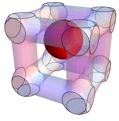
Figure 1: Hard-sphere particle trapped in a cuboid cell with cylindrical edges. One imagines a material consisting of many copies of such cells forming a spatially periodic structure. The cells are semi-porous in the sense that particles are prevented from escaping, and can yet partially penetrate into the neighbouring cells, thus allowing energy transfer through collisions among neighbouring particles. The likelihood of such collision events can be controlled by the geometry of the cell.

These systems combine the collisional dynamics of gases and the spatial structure of solids. There is therefore a natural distinction between the local dynamics, which deal with the interactions between the moving particles and the solid matrix of their confining cells, and the interacting dynamics, by which two moving particles in neighbouring cells perform an elastic collision. On the one hand, the local dynamics are characterized by a wall-collision frequency, $\nu_{\mathrm{W}}$, which depends on the geometry of the confining cell as well as on the kinetic energy of the moving particles through well known results of ergodic theory [7]. On the other hand, the interacting dynamics are characterized by the frequency of binary collisions, i.e. the frequency of collisions between neighbouring particles, denoted $\nu_{\mathrm{B}}$.

We assume that the scale separation, $\nu_{\mathrm{B}}\ll\nu_{\mathrm{W}}$, is achieved. This involves specific conditions which depend on the geometry of the confining cells, but which will not concern us here. This assumption is to say that individual particles typically perform many collisions with the solid matrix of their confining cells, rattling about their cages at higher frequency than that of binary collisions. As will be shown in the next section, in this regime, Liouville’s equation governing the time evolution of phase-space densities reduces to a master equation for the time evolution of local energies. The scale separation between the two collision frequencies $\nu_{\mathrm{B}}$ and $\nu_{\mathrm{W}}$ is the only parameter that controls the validity of this reduction. Moreover it becomes exact in the limit of vanishing binary collision frequency.

4 Statistical evolution

The phase-space probability density of the mechanical systems of $N$ confined hard spheres is specified by the distribution function $p_{N}(\bi{r}_{1},\bi{v}_{1},\dots,\bi{r}_{N},\bi{v}_{N})$, where $\bi{r}_{a}$ and $\bi{v}_{a}$, $a=1,\dots,N$, denote the $a$th particle position and velocity vectors. The index $a$ stands for the label of the confining cells. For our system, as is customary for hard sphere dynamics, this distribution satisfies a pseudo-Liouville equation [8], which is well defined in spite of the singularity of the hard-core interactions. This equation, which describes the time evolution of $p_{N}$ is composed of three types of terms: (i) the advection terms, which account for the displacement of the moving particles within their respective billiard cells; (ii) the wall collision terms, which account for the wall collision events, between the moving particles and the solid matrix of their confining cells; and (iii) the binary collision terms, which account for binary collision events, between moving particles belonging to neighbouring cells :

$$\partial_{t}p_{N}=\sum_{a=1}^{N}\left[-\bi{v}_{a}\cdot\partial_{\bi{r}_{a}}+K^{(a)}\right]p_{N}+\frac{1}{2}\sum_{a,b=1}^{N}B^{(a,b)}p_{N}\,.$$ (11)

The first two terms account for the motion of individual particles within their respective cells, whether free advection or wall collisions, and the third term is the binary collision operator which, written in terms of the relative positions $\bi{r}_{ab}$ and velocities $\bi{v}_{ab}$ of particles $a$ and $b$, and the unit vector $\hat{\bi{e}}_{ab}$ that connects them, is

$$\hbox to0.0pt{\hss${}B{}$}^{(a,b)}p_{N}(\dots,\bi{r}_{a},\bi{v}_{a},\dots,\bi{r}_{b},\bi{v}_{b},\dots)=$$

$$(2\rho_{\mathrm{m}})^{2}\int_{\hat{\bi{e}}_{ab}\cdot\bi{v}_{ab}>0}\/\mathrm{d}\/\hat{\bi{e}}_{ab}(\hat{\bi{e}}_{ab}\cdot\bi{v}_{ab})\Big{[}\delta(\bi{r}_{ab}-2\rho_{\mathrm{m}}\hat{\bi{e}}_{ab})$$

$$\times p_{N}\big{(}\dots,\bi{r}_{a},\bi{v}_{a}-\hat{\bi{e}}_{ab}(\hat{\bi{e}}_{ab}\cdot\bi{v}_{ab}),\dots,\bi{r}_{b},\bi{v}_{b}+\hat{\bi{e}}_{ab}(\hat{\bi{e}}_{ab}\cdot\bi{v}_{ab}),\dots\big{)}$$

$$-\delta(\bi{r}_{ab}+2\rho_{\mathrm{m}}\hat{\bi{e}}_{ab})p_{N}\big{(}\dots,\bi{r}_{a},\bi{v}_{a},\dots,\bi{r}_{b},\bi{v}_{b},\dots\big{)}\Big{]}\,.$$ (12)

4.1 Equilibrium states

Equilibrium states of equation (11) are product measures such as a Maxwellian distribution with inverse temperature $\beta$,

$$p_{N}^{(\mathrm{can})}(\bi{r}_{1},\bi{v}_{1},\dots,\bi{r}_{N},\bi{v}_{N})=\frac{1}{|\mathcal{L}(N)|}\left(\frac{m\beta}{2\pi}\right)^{\frac{3N}{2}}e^{-\frac{m}{2}\beta(v_{1}^{2}+\dots+v_{N}^{2})}\,,$$ (13)

where $|\mathcal{L}(N)|$ denotes the volume accessible to all $N$ particles, or micro-canonical measures of totally energy $E$,

$$p_{N}^{(\mathrm{mic})}(\bi{r}_{1},\bi{v}_{1},\dots,\bi{r}_{N},\bi{v}_{N})=\frac{\Gamma(\frac{3N}{2})E}{|\mathcal{L}(N)|}\left(\frac{m}{2\pi E}\right)^{\frac{3N}{2}}\delta\left(\frac{m}{2}\sum_{a}v_{a}^{2}-E\right)\,,$$ (14)

where the Gamma function is

$$\Gamma\left(\frac{3N}{2}\right)=\left\{\begin{array}[]{l@{\quad}l}(3N-2)!!\sqrt{2\pi}\,2^{-\frac{3N-2}{2}}\,,&N\,\mathrm{odd}\,,\\ (3N-2)!!2^{-\frac{3N-2}{2}}\,,&N\,\mathrm{even}\,.\\ \end{array}\right.$$ (15)

4.2 Local equilibrium states

Under the assumption that particles typically collide more often with the solid matrix of their confining cells than among nearest neighbours, the time-evolution (11) is dominated by the local terms so that the distribution $p_{N}$ rapidly evolves toward a local equilibrium distribution, which depends upon the energy variables $\{\epsilon_{1},\dots,\epsilon_{N}\}$ only.

We denote by $P_{N}(\epsilon_{1},\dots,\epsilon_{N},t)$ this object, invariant under the local evolution terms, defined in terms of the phase-space distribution function of the mechanical systems of $N$ confined particles $p_{N}(\bi{r}_{1},\bi{v}_{1},\dots,\bi{r}_{N},\bi{v}_{N},t)$ according to

$$P_{N}(\epsilon_{1},\dots,\epsilon_{N},t)\equiv\int\prod_{a=1}^{N}\/\mathrm{d}\/\bi{r}_{a}\/\mathrm{d}\/\bi{v}_{a}\delta\left(\epsilon_{a}-\frac{m}{2}v_{a}^{2}\right)p_{N}(\bi{r}_{1},\bi{v}_{1},\dots,\bi{r}_{N},\bi{v}_{N},t)\,.$$ (16)

Notice that the normalization of $p_{N}$ implies that of $P_{N}$.

In terms of the energy distributions, the corresponding equilibrium measures are

$$P_{N}^{(\mathrm{can})}(\epsilon_{1},\dots,\epsilon_{N})=\left(\frac{m\beta}{2\pi}\right)^{\frac{3N}{2}}\int\prod_{a=1}^{N}\/\mathrm{d}\/\bi{v}_{a}\delta\left(\epsilon_{a}-\frac{m}{2}v_{a}^{2}\right)e^{-\frac{m}{2}\beta(v_{1}^{2}+\dots+v_{N}^{2})}\,,$$

$$=\left(\frac{2\beta^{\frac{3}{2}}}{\sqrt{\pi}}\right)^{N}\sqrt{\epsilon_{1}\cdots\epsilon_{N}}e^{-\beta(\epsilon_{1}+\dots+\epsilon_{N})}\,.$$ (17)

$$P_{N}^{(\mathrm{mic})}(\epsilon_{1},\dots,\epsilon_{N})$$

$$=\Gamma\left(\frac{3N}{2}\right)E\left(\frac{m}{2\pi E}\right)^{\frac{3N}{2}}\int\prod_{a=1}^{N}\/\mathrm{d}\/\bi{v}_{a}\delta\left(\epsilon_{a}-\frac{m}{2}v_{a}^{2}\right)\delta\left(\frac{m}{2}\sum_{a}v_{a}^{2}-E\right)\,,$$

$$=\Gamma\left(\frac{3N}{2}\right)\left(\frac{2}{\sqrt{\pi}E}\right)^{N}\sqrt{\frac{\epsilon_{1}\cdots\epsilon_{N}}{E^{N}}}\delta\left(\frac{\epsilon_{1}}{E}+\dots+\frac{\epsilon_{N}}{E}-1\right)\,.$$ (18)

One can check that both these measures are normalized. We notice that the one- and two-point distribution of the canonical and micro-canonical measure (18) have the forms ($N\geq 3$)

$$P_{N}^{(\mathrm{can})}(\epsilon)=\frac{2\beta^{\frac{3}{2}}}{\sqrt{\pi}}\sqrt{\epsilon}e^{-\beta\epsilon}\,,$$ (19)

$$P_{N}^{(\mathrm{can})}(\epsilon_{a},\epsilon_{b})=\frac{4\beta^{3}}{\pi}\sqrt{\epsilon_{a}\epsilon_{b}}e^{-\beta(\epsilon_{a}+\epsilon_{b})}\,,$$ (20)

$$P_{N}^{(\mathrm{mic})}(\epsilon)=\frac{2}{\sqrt{\pi}E^{\frac{3}{2}}}\frac{\Gamma(\frac{3}{2}N)}{\Gamma[\frac{3}{2}(N-1)]}\sqrt{\epsilon}\left(1-\frac{\epsilon}{E}\right)^{\frac{3N-5}{2}}\,,$$ (21)

$$P_{N}^{(\mathrm{mic})}(\epsilon_{a},\epsilon_{b})=\frac{4\Gamma(\frac{3}{2}N)}{\pi E^{3}\Gamma(\frac{3}{2}N-3)}\sqrt{\epsilon_{a}\epsilon_{b}}\left(1-\frac{\epsilon_{a}}{E}-\frac{\epsilon_{b}}{E}\right)^{\frac{3N-8}{2}}\,.$$ (22)

The canonical ensemble marginals are straightforward. As of the micro-canonical ensemble, the marginals are obtained from the $N$-point distribution (18) by integrating out $N-2$ of the $N$ energy variables. The integration over the first of $N-2$ variables takes care of the delta function. Each subsequent integration has the form

$$\int_{0}^{x}\/\mathrm{d}\/y\,\sqrt{y}(x-y)^{a}\sim x^{\frac{3}{2}+a}\,,$$ (23)

where $x=1-\epsilon_{1}/N-\dots-\epsilon_{n}/N$. The successive values of $a$ are

$$\begin{array}[]{l@{\quad\mathrm{when}\,\mathrm{integrating}\,\mathrm{over} \quad}l}\frac{1}{2}&\,\epsilon_{N-1}\,,\\ 2&\,\epsilon_{N-2}\,,\\ \frac{7}{2}&\,\epsilon_{N-3}\,,\\ 5&\,\epsilon_{N-4}\,,\\ \end{array}$$ (24)

and so on until we obtain (22) after $N-2$ integrations.

Letting $E=3/2N\beta^{-1}$ into (21), and taking the limit $N\to\infty$, we recover

$$\lim_{N\to\infty}P_{N}^{(\mathrm{mic})}(\epsilon)=\frac{2\beta^{\frac{3}{2}}}{\sqrt{\pi}}\sqrt{\epsilon}\,e^{-\beta\epsilon}\,,$$ (25)

which is the one-particle distribution of the canonical measure (17).

The energy moments with respect to the one cell distributions (19), for the canonical ensemble, and (21), for the micro-canonical ensemble, are easily computed. Let $\langle.\rangle_{\mathrm{can}}$ and $\langle.\rangle_{\mathrm{mic}}$ denote the averages with respect to the distributions (19) and (21) at energy $E=3/2N\beta^{-1}$ respectively. The corresponding $n$th moments of the energy are

$$\langle(\beta\epsilon)^{n}\rangle_{\mathrm{can}} =\frac{2}{\sqrt{\pi}}\Gamma\left(\frac{3}{2}+n\right)\,,$$ (26)

$$=\frac{(2n+1)!!}{2^{n}}\,,$$

$$\langle(\beta\epsilon)^{n}\rangle_{\mathrm{mic}} =\frac{2}{\sqrt{\pi}}\left(\frac{3N}{2}\right)^{n}\frac{\Gamma(\frac{3}{2}+n)\Gamma(\frac{3}{2}N)}{\Gamma(\frac{3}{2}N+n)}\,,$$ (27)

$$=\frac{(2n+1)!!}{2^{n}}\frac{\left(\frac{3N}{2}\right)^{n}\Gamma(\frac{3}{2}N)}{\Gamma(\frac{3}{2}N+n)}\,.$$

In particular the first few moments are

$$\eqalign{\langle\beta\epsilon\rangle_{\mathrm{mic}}=\frac{3}{2}\,,\\ \langle(\beta\epsilon)^{2}\rangle_{\mathrm{mic}}=\frac{15}{4}\frac{3N}{3N+2}\,,\\ \langle(\beta\epsilon)^{3}\rangle_{\mathrm{mic}}=\frac{105}{8}\frac{9N^{2}}{(3N+4)(3N+2)}\,.\\ }$$ (28)

Thus only the first one is independent of $N$ and equal to its canonical counterpart. The remaining ones are only equal to their canonical counterparts up to $\mathcal{O}(1/N)$ corrections.

4.3 Local equilibrium closure

Taking the time-derivative of equation (16) and substituting equation (11), only the term involving energy exchanges between neighboring particles contribute :

$$\partial_{t}P_{N}(\epsilon_{1},\dots,\epsilon_{N},t) =\int\prod_{i=1}^{N}\/\mathrm{d}\/\bi{r}_{i}\/\mathrm{d}\/\bi{v}_{i}\delta\left(\epsilon_{i}-\frac{m}{2}v_{i}^{2}\right)\partial_{t}p_{N}(\bi{r}_{1},\bi{v}_{1},\dots,\bi{r}_{N},\bi{v}_{N},t)\,,$$ (29)

$$=\frac{1}{2}\sum_{a,b=1}^{N}\int\prod_{i=1}^{N}\/\mathrm{d}\/\bi{r}_{i}\/\mathrm{d}\/\bi{v}_{i}\delta\left(\epsilon_{i}-\frac{m}{2}v_{i}^{2}\right)\,B^{(a,b)}p_{N}(\bi{r}_{1},\bi{v}_{1},\dots,\bi{r}_{N},\bi{v}_{N},t)$$

The action of $B^{(a,b)}$ on $p_{N}$ is given according to equation (12). In order to obtain a closed equation for $P_{N}$, we assume that the distribution $p_{N}$ is a locally micro-canonical one, i.e. it depends only on the energy distribution and is thus given according to

$$p_{N}(\bi{r}_{1},\bi{v}_{1},\dots,\bi{r}_{N},\bi{v}_{N},t)=\frac{m^{N}}{(8\pi)^{N}|\mathcal{L}(N)|}\int\prod_{i=1}^{N}\/\mathrm{d}\/\epsilon_{i}\epsilon_{i}^{-1}\delta\left(v_{i}-\sqrt{\frac{2\epsilon_{i}}{m}}\right)P_{N}(\epsilon_{1},\dots,\epsilon_{N},t)\,.$$ (30)

The other prefactors are so chosen that this measure is normalized, viz.

$$\int\prod_{i=1}^{N}\/\mathrm{d}\/\bi{r}_{i}\/\mathrm{d}\/\bi{v}_{i}p_{N}(\bi{r}_{1},\bi{v}_{1},\dots,\bi{r}_{N},\bi{v}_{N},t)=1\,.$$ (31)

5 Master equation

The validity of equation (30) depends on the scale separation between the wall and binary collision frequencies which will be assumed throughout this article. This allows us to focus on the stochastic reduction of the energy exchange dynamics, considering the mesoscopic level description of the time evolution of probability densities as a stochastic evolution.

Indeed, substituting equation (30) into (12), we write the time evolution of local equilibrium distributions (29) in the form of the master equation (1), whose kernel $W$ can be identified from the computations above. The time evolution is thus specified by a master equation which accounts for the energy exchanges between neighbouring cells and makes no further reference to the collisional dynamics of confined hard spheres.

5.1 Derivation of the master equation

For each pair $(a,b)$ of neighbouring cells, we have a contribution to equation (29) of the form

$$\int\prod_{i=1}^{N}\/\mathrm{d}\/\bi{r}_{i}\/\mathrm{d}\/\bi{v}_{i}\delta\left(\epsilon_{i}-\frac{m}{2}v_{i}^{2}\right)B^{(a,b)}p_{N}(\{\bi{r}_{i},\bi{v}_{i}\},t)$$

$$=4\rho_{\mathrm{m}}^{2}\int\prod_{i=1}^{N}\/\mathrm{d}\/\bi{r}_{i}\/\mathrm{d}\/\bi{v}_{i}\int_{\hat{\bi{e}}_{ab}\cdot\bi{v}_{ab}>0}\/\mathrm{d}\/\hat{\bi{e}}_{ab}(\hat{\bi{e}}_{ab}\cdot\bi{v}_{ab})\delta\left(\epsilon_{i}-\frac{m}{2}v_{i}^{2}\right)$$ (32)

$$\hskip-28.45274pt\times\left[\delta(\bi{r}_{ab}-2\rho_{\mathrm{m}}\hat{\bi{e}}_{ab})p_{N}\big{(}\dots,\bi{v^{\prime}}_{a},\bi{v^{\prime}}_{b},\dots\big{)}-\delta(\bi{r}_{ab}+2\rho_{\mathrm{m}}\hat{\bi{e}}_{ab})p_{N}\big{(}\dots,\bi{v}_{a},\bi{v}_{b},\dots\big{)}\right]\,,$$

where $\bi{v^{\prime}}_{a}=\bi{v}_{a}-\hat{\bi{e}}_{ab}(\hat{\bi{e}}_{ab}\cdot\bi{v}_{ab})$ and $\bi{v^{\prime}}_{b}=\bi{v}_{b}+\hat{\bi{e}}_{ab}(\hat{\bi{e}}_{ab}\cdot\bi{v}_{ab})$. Substituting equation (30) into this expression, we have the contributions

$$4\rho_{\mathrm{m}}^{2}\frac{m^{N}}{(8\pi)^{N}|\mathcal{L}(N)|}\int\prod_{i=1}^{N}\/\mathrm{d}\/\bi{r}_{i}\/\mathrm{d}\/\bi{v}_{i}\delta\left(\epsilon_{i}-\frac{m}{2}v_{i}^{2}\right)\int_{\hat{\bi{e}}_{ab}\cdot\bi{v}_{ab}>0}\/\mathrm{d}\/\hat{\bi{e}}_{ab}(\hat{\bi{e}}_{ab}\cdot\bi{v}_{ab})$$ (33)

$$\hbox to0.0pt{\hss${}\times{}$}\Bigg{[}\delta(\bi{r}_{ab}-2\rho_{\mathrm{m}}\hat{\bi{e}}_{ab})\int\prod_{i=1}^{N}\/\mathrm{d}\/\tilde{\epsilon}_{i}\tilde{\epsilon}_{i}^{-1}\delta\left(v^{\prime}_{i}-\sqrt{\frac{2\tilde{\epsilon}_{i}}{m}}\right)P_{N}(\tilde{\epsilon}_{1},\dots,\tilde{\epsilon}_{N},t)$$

$$-\delta(\bi{r}_{ab}+2\rho_{\mathrm{m}}\hat{\bi{e}}_{ab})\int\prod_{i=1}^{N}\/\mathrm{d}\/\tilde{\epsilon}_{i}\tilde{\epsilon}_{i}^{-1}\delta\left(v_{i}-\sqrt{\frac{2\tilde{\epsilon}_{i}}{m}}\right)P_{N}(\tilde{\epsilon}_{1},\dots,\tilde{\epsilon}_{N},t)\Bigg{]}\,,$$

where $v^{\prime}_{i}=v_{i}$ for $i\neq a,b$ and

$$\eqalign{v^{\prime}_{a}=\sqrt{v_{a}^{2}-(\widehat{\bi{e}}_{ab}\cdot\bi{v}_{a})^{2}+(\widehat{\bi{e}}_{ab}\cdot\bi{v}_{b})^{2}}\,,\\ v^{\prime}_{b}=\sqrt{v_{b}^{2}+(\widehat{\bi{e}}_{ab}\cdot\bi{v}_{a})^{2}-(\widehat{\bi{e}}_{ab}\cdot\bi{v}_{b})^{2}}\,.}$$ (34)

Inserting factors $\int\/\mathrm{d}\/\eta\delta(\eta\pm m/2\big{[}(\widehat{\bi{e}}_{ab}\cdot\bi{v}_{a})^{2}-(\widehat{\bi{e}}_{ab}\cdot\bi{v}_{b})^{2}\big{]})$ in both of the terms between brackets, we write $\epsilon^{\prime}_{i}=\epsilon_{i}$, $i\neq a,b$, and $\epsilon^{\prime}_{a}=\epsilon_{a}+\eta$, $\epsilon^{\prime}_{b}=\epsilon_{b}-\eta$. The contribution (33) thus transforms into

$$4\rho_{\mathrm{m}}^{2}\frac{m^{N}}{(8\pi)^{N}|\mathcal{L}(N)|}\left(\frac{m}{2}\right)^{\frac{N}{2}}\int\prod_{i=1}^{N}\/\mathrm{d}\/\bi{r}_{i}\/\mathrm{d}\/\bi{v}_{i}\delta\left(\epsilon_{i}-\frac{m}{2}v_{i}^{2}\right)\int_{\hat{\bi{e}}_{ab}\cdot\bi{v}_{ab}>0}\/\mathrm{d}\/\hat{\bi{e}}_{ab}(\hat{\bi{e}}_{ab}\cdot\bi{v}_{ab})$$

$$\hbox to0.0pt{\hss${}\times{}$}\Bigg{[}\delta(\bi{r}_{ab}-2\rho_{\mathrm{m}}\hat{\bi{e}}_{ab})\int\/\mathrm{d}\/\eta\delta\left(\eta+\frac{m}{2}\big{[}(\widehat{\bi{e}}_{ab}\cdot\bi{v}_{a})^{2}-(\widehat{\bi{e}}_{ab}\cdot\bi{v}_{b})^{2}\big{]}\right)$$

$$\times\int\prod_{i=1}^{N}\/\mathrm{d}\/\tilde{\epsilon}_{i}\tilde{\epsilon}_{i}^{-1}\delta\big{(}\sqrt{}\epsilon^{\prime}_{i}-\sqrt{}\tilde{\epsilon}_{i}\big{)}P_{N}(\tilde{\epsilon}_{1},\dots,\tilde{\epsilon}_{N},t)$$

$$-\delta(\bi{r}_{ab}+2\rho_{\mathrm{m}}\hat{\bi{e}}_{ab})\int\/\mathrm{d}\/\eta\delta\left(\eta-\frac{m}{2}\big{[}(\widehat{\bi{e}}_{ab}\cdot\bi{v}_{a})^{2}-(\widehat{\bi{e}}_{ab}\cdot\bi{v}_{b})^{2}\big{]}\right)$$

$$\times\int\prod_{i=1}^{N}\/\mathrm{d}\/\tilde{\epsilon}_{i}\tilde{\epsilon}_{i}^{-1}\delta\big{(}\sqrt{}\epsilon_{i}-\sqrt{}\tilde{\epsilon}_{i}\big{)}P_{N}(\tilde{\epsilon}_{1},\dots,\tilde{\epsilon}_{N},t)\Bigg{]}\,,$$

$$=4\rho_{\mathrm{m}}^{2}\frac{m^{N}}{(8\pi)^{N}|\mathcal{L}(N)|}(2m)^{\frac{N}{2}}\int\prod_{i=1}^{N}\/\mathrm{d}\/\bi{r}_{i}\/\mathrm{d}\/\bi{v}_{i}\delta\left(\epsilon_{i}-\frac{m}{2}v_{i}^{2}\right)\int_{\hat{\bi{e}}_{ab}\cdot\bi{v}_{ab}>0}\/\mathrm{d}\/\hat{\bi{e}}_{ab}(\hat{\bi{e}}_{ab}\cdot\bi{v}_{ab})$$

$$\hbox to0.0pt{\hss${}\times{}$}\Bigg{[}\delta(\bi{r}_{ab}-2\rho_{\mathrm{m}}\hat{\bi{e}}_{ab})\int\/\mathrm{d}\/\eta\delta\left(\eta+\frac{m}{2}\big{[}(\widehat{\bi{e}}_{ab}\cdot\bi{v}_{a})^{2}-(\widehat{\bi{e}}_{ab}\cdot\bi{v}_{b})^{2}\big{]}\right)$$

$$\times\frac{1}{\sqrt{\epsilon^{\prime}_{1}\dots\epsilon^{\prime}_{N}}}P_{N}(\epsilon^{\prime}_{1},\dots,\epsilon^{\prime}_{N},t)$$

$$-\delta(\bi{r}_{ab}+2\rho_{\mathrm{m}}\hat{\bi{e}}_{ab})\int\/\mathrm{d}\/\eta\delta\left(\eta-\frac{m}{2}\big{[}(\widehat{\bi{e}}_{ab}\cdot\bi{v}_{a})^{2}-(\widehat{\bi{e}}_{ab}\cdot\bi{v}_{b})^{2}\big{]}\right)$$

$$\times\frac{1}{\sqrt{\epsilon_{1}\dots\epsilon_{N}}}P_{N}(\epsilon_{1},\dots,\epsilon_{N},t)\Bigg{]}\,,$$ (35)

where we used the identity $\/\mathrm{d}\/\epsilon/\epsilon=2\/\mathrm{d}\/\sqrt{\epsilon}/\sqrt{\epsilon}$ and carried out the $\tilde{\epsilon}$ integrations. We proceed by performing all the $\bi{r}_{i}$ and $\bi{v}_{i}$ integrations but for $i=a,b$. For the latter, we change variables from $(\bi{r}_{a},\bi{r}_{b})$ to $(\bi{R}_{ab},\bi{r}_{ab})$, the center of mass and relative coordinates respectively. The latter integration can be carried out, with outcome $\bi{r}_{ab}=\pm 2\rho_{\mathrm{m}}\hat{\bi{e}}_{ab}$. We are thus led to contributions

$$\frac{\rho_{\mathrm{m}}^{2}m^{3}}{8\pi^{2}|\mathcal{L}(2)|}\int\/\mathrm{d}\/\bi{R}_{ab}\/\mathrm{d}\/\bi{v}_{a}\/\mathrm{d}\/\bi{v}_{b}\delta\left(\epsilon_{a}-\frac{m}{2}v_{a}^{2}\right)\delta\left(\epsilon_{b}-\frac{m}{2}v_{b}^{2}\right)\int_{\hat{\bi{e}}_{ab}\cdot\bi{v}_{ab}>0}\/\mathrm{d}\/\hat{\bi{e}}_{ab}(\hat{\bi{e}}_{ab}\cdot\bi{v}_{ab})$$

$$\times\Bigg{[}\frac{1}{\sqrt{(\epsilon_{a}+\eta)(\epsilon_{b}-\eta)}}\int\/\mathrm{d}\/\eta\delta\left(\eta+\frac{m}{2}\big{[}(\widehat{\bi{e}}_{ab}\cdot\bi{v}_{a})^{2}-(\widehat{\bi{e}}_{ab}\cdot\bi{v}_{b})^{2}\big{]}\right)$$

$$\times P_{N}(\epsilon_{1},\dots,\epsilon_{a}+\eta,\epsilon_{b}-\eta,\dots,\epsilon_{N},t)$$

$$-\frac{1}{\sqrt{\epsilon_{a}\epsilon_{b}}}\int\/\mathrm{d}\/\eta\delta\left(\eta-\frac{m}{2}\big{[}(\widehat{\bi{e}}_{ab}\cdot\bi{v}_{a})^{2}-(\widehat{\bi{e}}_{ab}\cdot\bi{v}_{b})^{2}\big{]}\right)P_{N}(\epsilon_{1},\dots,\epsilon_{N},t)\Bigg{]}\,.$$ (36)

Notice that we have made the assumption that the position integrals of the $N-2$ particles not involved in the collision factorise:

$$|\mathcal{L}(N)|=|\mathcal{L}(2)||\mathcal{L}(N-2)|\,.$$ (37)

Though this is an approximation, it becomes exact under the assumption of scale separation, which implies $|\mathcal{L}(N)|=|\mathcal{L}(1)|^{N}$. Comparing the above expression to equation (1), we identify the kernels associated with the gain and loss terms,

$$W(\epsilon_{a}+\eta,\epsilon_{b}-\eta|\epsilon_{a},\epsilon_{b})=\frac{\rho_{\mathrm{m}}^{2}m^{3}}{8\pi^{2}|\mathcal{L}(2)|}\int\/\mathrm{d}\/\Omega\/\mathrm{d}\/\bi{R}$$

$$\times\frac{1}{\sqrt{(\epsilon_{a}+\eta)(\epsilon_{b}-\eta)}}\int_{\widehat{\bi{e}}_{ab}\cdot\bi{v}_{ab}>0}\/\mathrm{d}\/\bi{v_{a}}\/\mathrm{d}\/\bi{v_{b}}(\widehat{\bi{e}}_{ab}\cdot\bi{v}_{ab})\delta\left(\epsilon_{a}-\frac{m}{2}v_{a}^{2}\right)$$

$$\times\delta\left(\epsilon_{b}-\frac{m}{2}v_{b}^{2}\right)\delta\left(\eta+\frac{m}{2}\big{[}(\widehat{\bi{e}}_{ab}\cdot\bi{v}_{a})^{2}-(\widehat{\bi{e}}_{ab}\cdot\bi{v}_{b})^{2}\big{]}\right)\,,$$

$$\hbox to0.0pt{\hss${}={}$}-\frac{\rho_{\mathrm{m}}^{2}m^{3}}{8\pi^{2}|\mathcal{L}(2)|}\int\/\mathrm{d}\/\Omega\/\mathrm{d}\/\bi{R}$$

$$\times\frac{1}{\sqrt{(\epsilon_{a}+\eta)(\epsilon_{b}-\eta)}}\int_{\widehat{\bi{e}}_{ab}\cdot\bi{v^{\prime}}_{ab}<0}\/\mathrm{d}\/\bi{v^{\prime}_{a}}\/\mathrm{d}\/\bi{v^{\prime}_{b}}(\widehat{\bi{e}}_{ab}\cdot\bi{v^{\prime}}_{ab})\delta\left(\epsilon_{a}+\eta-\frac{m}{2}{v^{\prime}_{a}}^{2}\right)$$

$$\times\delta\left(\epsilon_{b}-\eta-\frac{m}{2}{v^{\prime}_{b}}^{2}\right)\delta\left(\eta+\frac{m}{2}\big{[}(\widehat{\bi{e}}_{ab}\cdot\bi{v^{\prime}}_{b})^{2}-(\widehat{\bi{e}}_{ab}\cdot\bi{v^{\prime}}_{a})^{2}\big{]}\right)\,,$$ (38)

$$W(\epsilon_{a},\epsilon_{b}|\epsilon_{a}-\eta,\epsilon_{b}+\eta)=\frac{\rho_{\mathrm{m}}^{2}m^{3}}{8\pi^{2}|\mathcal{L}(2)|}\int\/\mathrm{d}\/\Omega\/\mathrm{d}\/\bi{R}$$

$$\times\frac{1}{\sqrt{\epsilon_{a}\epsilon_{b}}}\int_{\widehat{\bi{e}}_{ab}\cdot\bi{v}_{ab}>0}\/\mathrm{d}\/\bi{v_{a}}\/\mathrm{d}\/\bi{v_{b}}(\widehat{\bi{e}}_{ab}\cdot\bi{v}_{ab})\delta\left(\epsilon_{a}-\frac{m}{2}v_{a}^{2}\right)$$

$$\times\delta\left(\epsilon_{b}-\frac{m}{2}v_{b}^{2}\right)\delta\left(\eta-\frac{m}{2}\big{[}(\widehat{\bi{e}}_{ab}\cdot\bi{v}_{a})^{2}-(\widehat{\bi{e}}_{ab}\cdot\bi{v}_{b})^{2}\big{]}\right)\,,$$ (39)

where, in the expression of the gain term (38), we changed the post-collisional velocity variables $(\bi{v}_{a},\bi{v}_{b})$ to the pre-collisional velocities $(\bi{v^{\prime}}_{a},\bi{v^{\prime}}_{b})$.

Without loss of generality, we assume $\bi{v}_{a}$ and $\bi{v}_{b}$ are measured with respect to referentials whose $z$-axis point along the unit vector $\widehat{\bi{e}}_{ab}$. In such a case, we have $\widehat{\bi{e}}_{ab}\cdot\bi{v}_{a}=v_{a}\cos\phi_{a}$ and $\widehat{\bi{e}}_{ab}\cdot\bi{v}_{b}=v_{b}\cos\phi_{b}$. Thus the volume integral $\int\/\mathrm{d}\/\Omega\/\mathrm{d}\/\bi{R}$ decouples from the velocity integrals which yield

$$-\int_{\widehat{\bi{e}}_{ab}\cdot\bi{v^{\prime}}_{ab}<0}\/\mathrm{d}\/\bi{v^{\prime}_{a}}\/\mathrm{d}\/\bi{v^{\prime}_{b}}(\widehat{\bi{e}}_{ab}\cdot\bi{v^{\prime}}_{ab})\delta\left(\epsilon_{a}+\eta-\frac{m}{2}{v^{\prime}_{a}}^{2}\right)\delta\left(\epsilon_{b}-\eta-\frac{m}{2}{v^{\prime}_{b}}^{2}\right)$$ (40)

$$\times\delta\left(\eta+\frac{m}{2}\big{[}(\widehat{\bi{e}}_{ab}\cdot\bi{v^{\prime}}_{b})^{2}-(\widehat{\bi{e}}_{ab}\cdot\bi{v^{\prime}}_{a})^{2}\big{]}\right)$$

$$\hbox to0.0pt{\hss${}={}$}\pi^{2}\left(\frac{2}{m}\right)^{\frac{7}{2}}\sqrt{\epsilon_{a}^{\prime}\epsilon^{\prime}_{b}}\int_{\sqrt{\epsilon^{\prime}_{b}}x_{b}>\sqrt{\epsilon^{\prime}_{a}}x_{a}}\/\mathrm{d}\/x_{a}\/\mathrm{d}\/x_{b}(\sqrt{\epsilon^{\prime}_{b}}x_{b}-\sqrt{\epsilon^{\prime}_{a}}x_{a})\delta(\eta+[\epsilon^{\prime}_{b}x_{b}^{2}-\epsilon^{\prime}_{a}x_{a}^{2}])\,,$$

$$\int_{\widehat{\bi{e}}_{ab}\cdot\bi{v}_{ab}>0}\/\mathrm{d}\/\bi{v_{a}}\/\mathrm{d}\/\bi{v_{b}}(\widehat{\bi{e}}_{ab}\cdot\bi{v}_{ab})\delta\left(\epsilon_{a}-\frac{m}{2}v_{a}^{2}\right)\delta\left(\epsilon_{b}-\frac{m}{2}v_{b}^{2}\right)$$ (41)

$$\times\delta\left(\eta-\frac{m}{2}\big{[}(\widehat{\bi{e}}_{ab}\cdot\bi{v}_{a})^{2}-(\widehat{\bi{e}}_{ab}\cdot\bi{v}_{b})^{2}\big{]}\right)$$

$$\hbox to0.0pt{\hss${}={}$}\pi^{2}\left(\frac{2}{m}\right)^{\frac{7}{2}}\sqrt{\epsilon_{a}\epsilon_{b}}\int_{\sqrt{\epsilon_{a}}x_{a}>\sqrt{\epsilon_{b}}x_{b}}\/\mathrm{d}\/x_{a}\/\mathrm{d}\/x_{b}(\sqrt{\epsilon_{a}}x_{a}-\sqrt{\epsilon_{b}}x_{b})\delta(\eta-[\epsilon_{a}x_{a}^{2}-\epsilon_{b}x_{b}^{2}])\,.$$

Notice that the two integrals are identical upon exchanging the roles of $a$ and $b$ and $\eta\to-\eta$, except for the energies $\epsilon_{a}^{\prime}=\epsilon_{a}+\eta$ and $\epsilon_{b}^{\prime}=\epsilon_{b}-\eta$ in the expression (40). Thus the kernels (38)-(39) have expressions

$$W(\epsilon_{a}+\eta,\epsilon_{b}-\eta|\epsilon_{a},\epsilon_{b})=\sqrt{\frac{2}{m}}\frac{\rho_{\mathrm{m}}^{2}}{|\mathcal{L}(2)|}\int\/\mathrm{d}\/\Omega\/\mathrm{d}\/\bi{R}$$

$$\times\int_{\sqrt{\epsilon^{\prime}_{b}}x_{b}>\sqrt{\epsilon^{\prime}_{a}}x_{a}}\/\mathrm{d}\/x_{a}\/\mathrm{d}\/x_{b}(\sqrt{\epsilon^{\prime}_{b}}x_{b}-\sqrt{\epsilon^{\prime}_{a}}x_{a})\delta(\eta+[\epsilon^{\prime}_{b}x_{b}^{2}-\epsilon^{\prime}_{a}x_{a}^{2}])\,,$$ (42)

$$W(\epsilon_{a},\epsilon_{b}|\epsilon_{a}-\eta,\epsilon_{b}+\eta)=\sqrt{\frac{2}{m}}\frac{\rho_{\mathrm{m}}^{2}}{|\mathcal{L}(2)|}\int\/\mathrm{d}\/\Omega\/\mathrm{d}\/\bi{R}$$

$$\times\int_{\sqrt{\epsilon_{a}}x_{a}>\sqrt{\epsilon_{b}}x_{b}}\/\mathrm{d}\/x_{a}\/\mathrm{d}\/x_{b}(\sqrt{\epsilon_{a}}x_{a}-\sqrt{\epsilon_{b}}x_{b})\delta(\eta-[\epsilon_{a}x_{a}^{2}-\epsilon_{b}x_{b}^{2}])\,.$$ (43)

Notice the symmetry between the kernels of the gain and loss terms, i.e.

$$W(\epsilon_{a}+\eta,\epsilon_{b}-\eta|\epsilon_{a},\epsilon_{b})=W(\epsilon^{\prime}_{a},\epsilon^{\prime}_{b}|\epsilon^{\prime}_{a}-\eta,\epsilon^{\prime}_{b}+\eta)\,.$$ (44)

This is however no to say that the kernels are symmetric. In fact

$$W(\epsilon_{a}+\eta,\epsilon_{b}-\eta|\epsilon_{a},\epsilon_{b})\neq W(\epsilon_{a},\epsilon_{b}|\epsilon_{a}+\eta,\epsilon_{b}-\eta)\,,$$ (45)

which can be seen by rewriting equation (42) directly in terms of $\epsilon_{a}$ and $\epsilon_{b}$ :

$$W(\epsilon_{a}+\eta,\epsilon_{b}-\eta|\epsilon_{a},\epsilon_{b})=\sqrt{\frac{2}{m}}\frac{\rho_{\mathrm{m}}^{2}}{|\mathcal{L}(2)|}\int\/\mathrm{d}\/\Omega\/\mathrm{d}\/\bi{R}\sqrt{\frac{\epsilon_{a}\epsilon_{b}}{(\epsilon_{a}+\eta)(\epsilon_{b}-\eta)}}$$

$$\times\int_{\sqrt{\epsilon_{a}}x_{a}>\sqrt{\epsilon_{b}}x_{b}}\/\mathrm{d}\/x_{a}\/\mathrm{d}\/x_{b}(\sqrt{\epsilon_{a}}x_{a}-\sqrt{\epsilon_{b}}x_{b})\delta(\eta+[\epsilon_{a}x_{a}^{2}-\epsilon_{b}x_{b}^{2}])\,.$$ (46)

The symmetry is therefore the following

$$\sqrt{(\epsilon_{a}+\eta)(\epsilon_{b}-\eta)}W(\epsilon_{a}+\eta,\epsilon_{b}-\eta|\epsilon_{a},\epsilon_{b})=\sqrt{\epsilon_{a}\epsilon_{b}}W(\epsilon_{a},\epsilon_{b}|\epsilon_{a}+\eta,\epsilon_{b}-\eta)\,,$$ (47)

consistent with the form of the equilibrium distributions (17). This is to say that, despite the lack of symmetry (45), detailed balance is recovered:

$$\hbox to0.0pt{\hss${}W{}$}(\epsilon_{a}+\eta,\epsilon_{b}-\eta|\epsilon_{a},\epsilon_{b})P^{(\mathrm{eq})}(\dots,\epsilon_{a}+\eta,\epsilon_{b}-\eta,\dots)$$ (48)

$$=W(\epsilon_{a},\epsilon_{b}|\epsilon_{a}+\eta,\epsilon_{b}-\eta)P^{(\mathrm{eq})}(\dots,\epsilon_{a},\epsilon_{b},\dots)\,.$$

Therefore $\partial_{t}P^{(\mathrm{eq})}(\epsilon_{1},\dots\epsilon_{N})=0$, as must be.

5.2 Computation of the loss term

Going back to equation (43), we can write

$$\hbox to0.0pt{\hss${}\delta{}$}(\eta-\epsilon_{a}x_{a}^{2}+\epsilon_{b}x_{b}^{2})$$ (49)

$$=\frac{1}{2\sqrt{\epsilon_{a}(\eta+\epsilon_{b}x_{b}^{2})}}\left[\delta\left(x_{a}-\sqrt{\frac{\eta+\epsilon_{b}x_{b}^{2}}{\epsilon_{a}}}\right)+\delta\left(x_{a}+\sqrt{\frac{\eta+\epsilon_{b}x_{b}^{2}}{\epsilon_{a}}}\right)\right]\,.$$

The validity of this expression requires $\eta+\epsilon_{b}x_{b}^{2}>0$, which is satisfied whenever $\eta>0$ or

$$\mathrm{abs}(x_{b})>\sqrt{\frac{-\eta}{\epsilon_{b}}}\,,\quad\mathrm{if}\,\eta<0\,.$$ (50)

Provided this condition is fulfilled, we can carry out the $x_{a}$-integration in equation (43). Considering the arguments of the delta functions in equation (49), the result of the integration would be trivial unless

$$\eta+\epsilon_{b}x_{b}^{2}<\epsilon_{a}\Leftrightarrow\mathrm{abs}(x_{b})<\sqrt{\frac{\epsilon_{a}-\eta}{\epsilon_{b}}}\,.$$ (51)

The bounds of the $x_{b}$-integral are respectively

$$\eqalign{x_{\mathrm{min}}\equiv\mathrm{max}[-1,-\sqrt{(\epsilon_{a}-\eta)/\epsilon_{b}}],\\ x_{\mathrm{max}}\equiv\mathrm{min}[1,\sqrt{(\epsilon_{a}-\eta)/\epsilon_{b}}].}$$ (52)

which is

$$x_{\mathrm{max}}=-x_{\mathrm{min}}=\left\{\begin{array}[]{l@{\quad}l}1\,,&\eta<\epsilon_{a}-\epsilon_{b}\,,\\ \sqrt{\frac{\epsilon_{a}-\eta}{\epsilon_{b}}}\,,&\eta>\epsilon_{a}-\epsilon_{b}\,.\end{array}\right.$$ (53)

5.2.1 $\eta>0$:

The condition on the integration domain transposes into the Heaviside step function with arguments $\pm\sqrt{\eta+\epsilon_{b}x_{b}^{2}}-\sqrt{\epsilon_{b}}x_{b}$. Only the positive sign contributes to the kernel (43). Leaving aside the prefactors, we have

$$W(\epsilon_{a},\epsilon_{b}|\epsilon_{a}-\eta,\epsilon_{b}+\eta) \sim\frac{1}{2\sqrt{\epsilon_{a}}}\int_{x_{\mathrm{min}}}^{x_{\mathrm{max}}}\/\mathrm{d}\/x_{b}\left(1-\frac{\sqrt{\epsilon_{b}}x_{b}}{\sqrt{\eta+\epsilon_{b}x_{b}^{2}}}\right)\,,$$ (54)

$$=\frac{1}{\sqrt{\epsilon_{a}}}x_{\mathrm{max}}\,,$$

where we used the symmetry $x_{\mathrm{min}}=-x_{\mathrm{max}}$. Using equation (53), we have

$$\hbox to0.0pt{\hss${}W{}$}(\epsilon_{a},\epsilon_{b}|\epsilon_{a}-\eta,\epsilon_{b}+\eta)\sim\left\{\begin{array}[]{l@{\quad}l}\frac{1}{\sqrt{\epsilon_{a}}}\,,&0<\eta<\epsilon_{a}-\epsilon_{b}\quad(\mathrm{if}\,\epsilon_{a}>\epsilon_{b})\,,\\ \sqrt{\frac{\epsilon_{a}-\eta}{\epsilon_{a}\epsilon_{b}}}\,,&0\leq\epsilon_{a}-\epsilon_{b}<\eta<\epsilon_{a}\,,\end{array}\right.$$ (55)

5.2.2 $\eta<0$:

In this case, the $x_{b}$-integral in (43) splits into two separate integrals, the first from $x_{\mathrm{min}}$, as defined above, to $-x_{\mathrm{mid}}$, and the second from $x_{\mathrm{mid}}$ to $x_{\mathrm{max}}$, with

$$x_{\mathrm{mid}}\equiv\sqrt{\frac{-\eta}{\epsilon_{b}}}\,.$$ (56)

Note that the bounds are well ordered : we always have $x_{\mathrm{mid}}\leq x_{\mathrm{max}}$.

The terms contributing to the kernel are $\pm\sqrt{\eta+\epsilon_{b}x_{b}^{2}}-\sqrt{\epsilon_{b}}x_{b}$ for $x_{b}<0$. We have

$$W(\epsilon_{a},\epsilon_{b}|\epsilon_{a}-\eta,\epsilon_{b}+\eta) \sim\frac{1}{2\sqrt{\epsilon_{a}}}\int_{-x_{\mathrm{max}}}^{-x_{\mathrm{mid}}}\/\mathrm{d}\/x_{b}\left(-2\frac{\sqrt{\epsilon_{b}}x_{b}}{\sqrt{\eta+\epsilon_{b}x_{b}^{2}}}\right)\,,$$ (57)

$$=\sqrt{\frac{\eta+\epsilon_{b}x_{\mathrm{max}}^{2}}{\epsilon_{a}\epsilon_{b}}}-\sqrt{\frac{\eta+\epsilon_{b}x_{\mathrm{mid}}^{2}}{\epsilon_{a}\epsilon_{b}}}$$

Substituting the expressions of $x_{\mathrm{max}}$ and $x_{\mathrm{mid}}$, we find

$$W(\epsilon_{a},\epsilon_{b}|\epsilon_{a}-\eta,\epsilon_{b}+\eta)\sim\left\{\begin{array}[]{l@{\quad}l}\frac{1}{\sqrt{\epsilon_{b}}}\,,&\epsilon_{a}-\epsilon_{b}<\eta<0\quad(\mathrm{if}\,\epsilon_{b}>\epsilon_{a})\,,\\ \sqrt{\frac{\eta+\epsilon_{b}}{\epsilon_{a}\epsilon_{b}}}\,,&-\epsilon_{b}<\eta<\epsilon_{a}-\epsilon_{b}\leq 0\,.\end{array}\right.$$ (58)

5.2.3 To summarize:

We can write for the loss term:

$$W(\epsilon_{a},\epsilon_{b}|\epsilon_{a}-\eta,\epsilon_{b}+\eta)=\sqrt{\frac{2}{m}}\frac{\rho_{\mathrm{m}}^{2}}{|\mathcal{L}(2)|}\int\/\mathrm{d}\/\Omega\/\mathrm{d}\/\bi{R}$$ (59)

$$\hskip 56.9055pt\times\left\{\begin{array}[]{l@{\quad}l}\sqrt{\frac{\epsilon_{a}-\eta}{\epsilon_{a}\epsilon_{b}}}\,,&\mathrm{max}(0,\epsilon_{a}-\epsilon_{b})<\eta<\epsilon_{a}\,,\\ \frac{1}{\sqrt{\mathrm{max}(\epsilon_{a},\epsilon_{b})}}\,,&\mathrm{min}(0,\epsilon_{a}-\epsilon_{b})<\eta<\mathrm{max}(0,\epsilon_{a}-\epsilon_{b})\,,\\ \sqrt{\frac{\epsilon_{b}+\eta}{\epsilon_{a}\epsilon_{b}}}\,,&-\epsilon_{b}<\eta<\mathrm{min}(0,\epsilon_{a}-\epsilon_{b})\,.\end{array}\right.$$ (63)

It is readily checked that $W$ is symmetric under exchanging $\epsilon_{a}\leftrightarrow\epsilon_{b}$ and $\eta\to-\eta$, as it must be, and has the inverse units of time times energy.

5.3 Gain term

Going through the same steps as in Section 5.2 above, we find for the gain term:

$$W(\epsilon_{a}+\eta,\epsilon_{b}-\eta|\epsilon_{a},\epsilon_{b})=\sqrt{\frac{2}{m}}\frac{\rho_{\mathrm{m}}^{2}}{|\mathcal{L}(2)|}\int\/\mathrm{d}\/\Omega\/\mathrm{d}\/\bi{R}$$ (64)

$$\hskip 56.9055pt\times\left\{\begin{array}[]{l@{\quad}l}\frac{1}{\sqrt{\epsilon_{a}+\eta}}\,,&\mathrm{max}(\epsilon_{b}-\epsilon_{a},0)<\eta<\epsilon_{b}\,,\\ \sqrt{\frac{\mathrm{min}(\epsilon_{a},\epsilon_{b})}{(\epsilon_{a}+\eta)(\epsilon_{b}-\eta)}}\,,&\mathrm{min}(\epsilon_{b}-\epsilon_{a},0)<\eta<\mathrm{max}(\epsilon_{b}-\epsilon_{a},0)\,,\\ \frac{1}{\sqrt{\epsilon_{b}-\eta}}\,,&-\epsilon_{a}<\eta<\mathrm{min}(\epsilon_{b}-\epsilon_{a},0)\,.\end{array}\right.$$ (68)

Comparing with equation (59), we check that the loss and gain terms have the symmetry of equation (48).

6 Collision frequency and heat conductivity

We can rescale time by a factor $(4\rho_{\mathrm{m}})^{2}/(\sqrt{m\pi}|\mathcal{L}(2)|)\int\/\mathrm{d}\/\Omega\/\mathrm{d}\/\bi{R}$, which amounts to converting the time units to units of the inverse square root of energy. The expression of the kernel thus simplifies to:

$$W(\epsilon_{a},\epsilon_{b}|\epsilon_{a}-\eta,\epsilon_{b}+\eta)=$$ (69)

$$\hskip 56.9055pt\sqrt{\frac{\pi}{8}}\times\left\{\begin{array}[]{l@{\quad}l}\sqrt{\frac{\epsilon_{b}+\eta}{\epsilon_{a}\epsilon_{b}}}\,,&-\epsilon_{b}<\eta<\mathrm{min}(0,\epsilon_{a}-\epsilon_{b})\,,\\ \frac{1}{\sqrt{\mathrm{max}(\epsilon_{a},\epsilon_{b})}}\,,&\mathrm{min}(0,\epsilon_{a}-\epsilon_{b})<\eta<\mathrm{max}(0,\epsilon_{a}-\epsilon_{b})\,,\\ \sqrt{\frac{\epsilon_{a}-\eta}{\epsilon_{a}\epsilon_{b}}}\,,&\mathrm{max}(0,\epsilon_{a}-\epsilon_{b})<\eta<\epsilon_{a}\,.\end{array}\right.$$ (73)

A graphical representation of this function is displayed in figure 2.

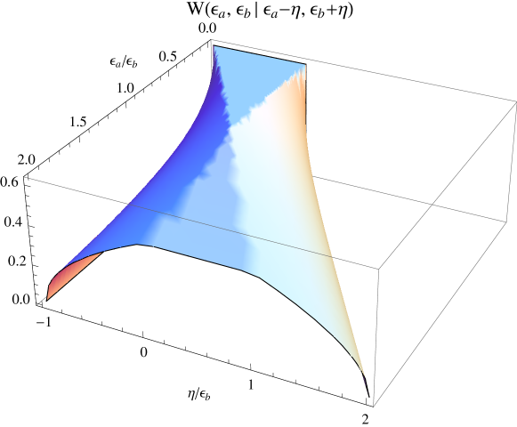
Figure 2: Stochastic kernel (69) associated with the probability of an energy exchange $\eta$ between two cells at energies $\epsilon_{a}$ and $\epsilon_{b}$.

The rate of energy exchange (2) is

$$\nu(\epsilon_{a},\epsilon_{b})=\frac{\sqrt{2\pi}}{12}\times\left\{\begin{array}[]{l@{\quad}l}\frac{\epsilon_{a}+3\epsilon_{b}}{\sqrt{\epsilon_{b}}}\,,&\epsilon_{b}\geq\epsilon_{a}\,,\\ \frac{3\epsilon_{a}+\epsilon_{b}}{\sqrt{\epsilon_{a}}}\,,&\epsilon_{a}\geq\epsilon_{b}\,,\\ \end{array}\right.$$ (76)

with equilibrium average taken with respect to the measure (17),

$$\nu_{\mathrm{B}}=\frac{4}{\pi T^{3}}\int\/\mathrm{d}\/\epsilon_{a}\/\mathrm{d}\/\epsilon_{b}\nu(\epsilon_{a},\epsilon_{b})\sqrt{\epsilon_{a}\epsilon_{b}}e^{-(\epsilon_{a}+\epsilon_{b})/T}=\sqrt{T}\,.$$ (77)

The micro-canonical average of the collision frequency is the quantity

$$\nu_{\mathrm{B}}(N)=\int\/\mathrm{d}\/\epsilon_{a}\/\mathrm{d}\/\epsilon_{b}\nu(\epsilon_{a},\epsilon_{b})P^{(\mathrm{mic})}_{N}(\epsilon_{a},\epsilon_{b})=\sqrt{T}[1+\mathcal{O}(1/N)]\,.$$ (78)

The amount of heat transfer is

$$j(\epsilon_{a},\epsilon_{b})=\frac{\sqrt{2\pi}}{24}(\epsilon_{a}-\epsilon_{b})\times\left\{\begin{array}[]{l@{\quad}l}\frac{\epsilon_{a}+3\epsilon_{b}}{\sqrt{\epsilon_{b}}}\,,&\epsilon_{b}\geq\epsilon_{a}\,,\\ \frac{3\epsilon_{a}+\epsilon_{b}}{\sqrt{\epsilon_{a}}}\,,&\epsilon_{a}\geq\epsilon_{b}\,,\\ \end{array}\right.$$ (81)

which is equivalent to

$$j(\epsilon_{a},\epsilon_{b})=\frac{1}{2}(\epsilon_{a}-\epsilon_{b})\nu(\epsilon_{a},\epsilon_{b}).$$ (82)

Thus, with the help of the identity

$$\frac{1}{\pi T^{5}}\int\/\mathrm{d}\/\epsilon_{a}\/\mathrm{d}\/\epsilon_{b}\nu(\epsilon_{a},\epsilon_{b})(\epsilon_{a}-\epsilon_{b})^{2}\sqrt{\epsilon_{a}\epsilon_{b}}e^{-(\epsilon_{a}+\epsilon_{b})/T}=\sqrt{T}\,,$$ (83)

we can compute the average of the heat current weighted by $(\epsilon_{a}-\epsilon_{b})/2$ with respect to local thermal equilibrium measure to obtain the heat conductivity:

$$\kappa =\frac{2}{\pi T^{5}}\int\/\mathrm{d}\/\epsilon_{a}\/\mathrm{d}\/\epsilon_{b}j(\epsilon_{a},\epsilon_{b})(\epsilon_{a}-\epsilon_{b})\sqrt{\epsilon_{a}\epsilon_{b}}e^{-(\epsilon_{a}+\epsilon_{b})/T}\,,$$ (84)

$$=\frac{1}{\pi T^{5}}\int\/\mathrm{d}\/\epsilon_{a}\/\mathrm{d}\/\epsilon_{b}\nu(\epsilon_{a},\epsilon_{b})(\epsilon_{a}-\epsilon_{b})^{2}\sqrt{\epsilon_{a}\epsilon_{b}}e^{-(\epsilon_{a}+\epsilon_{b})/T}\,,$$

$$=\sqrt{T}\,,$$

The ratio between the heat conductivity and collision frequency is therefore unity, as announced (5).

The same result is obtained from the equilibrium average of the second moment of the heat transfer (7):

$$h(\epsilon_{a},\epsilon_{b})=\frac{\sqrt{2\pi}}{420}\left\{\begin{array}[]{l@{\quad}l}\frac{35\epsilon_{b}^{2}(\epsilon_{b}-\epsilon_{a})+21\epsilon_{b}\epsilon_{a}^{2}+11\epsilon_{a}^{3}}{\sqrt{\epsilon_{b}}}\,,&\epsilon_{b}\geq\epsilon_{a}\,,\\ \frac{35\epsilon_{a}^{2}(\epsilon_{a}-\epsilon_{b})+21\epsilon_{a}\epsilon_{b}^{2}+11\epsilon_{b}^{3}}{\sqrt{\epsilon_{a}}}\,,&\epsilon_{a}\geq\epsilon_{b}\,,\end{array}\right.$$ (85)

which yields an alternative derivation of the heat conductivity by taking the equilibrium average of this quantity:

$$\kappa =\frac{2}{\pi T^{5}}\int\/\mathrm{d}\/\epsilon_{a}\/\mathrm{d}\/\epsilon_{b}h(\epsilon_{a},\epsilon_{b})\sqrt{\epsilon_{a}\epsilon_{b}}e^{-(\epsilon_{a}+\epsilon_{b})/T}\,,$$ (86)

$$=\sqrt{T}\,.$$

This result is universal for three-dimensional systems in the sense that it holds for confined particles interacting through hardcore collisions, independent of the shape of the confining cells and temperature, at least so long as the local dynamics is ergodic on the constant energy surface.

7 Numerical scheme

Equation (5) can be verified by direct numerical computations of the master equation (1) according to the scheme described in [6], based on Gillespie’s algorithm [9, 10]. We recall that the Monte-Carlo step necessitates two random trials. The first random number determines the time that will elapse until the next energy exchange event. The second one determines which one out of all the possible pairs of cells will perform an exchange of energy and how much energy will be exchanged between them.

Thus let $\xi$ and $\chi$ be these two random numbers, uniformly distributed on the unit interval and let us consider an array –whether one-, two- or three-dimensional– of $N$ pairs of energy variables $\Big{\{}\epsilon_{1}^{(i)},\epsilon_{2}^{(i)}\Big{\}}_{i=1}^{N}$.

The first random number, $\xi$, determines the time to the next energy exchange event, denoted $\tau$, according to the Poisson distribution whose relaxation rate is given by the sum of the respective exchange rates $\nu\Big{(}\epsilon_{1}^{(i)},\epsilon_{2}^{(i)}\Big{)}$ between pairs of energies $\Big{\{}\epsilon_{1}^{(i)},\epsilon_{2}^{(i)}\Big{\}}$,

$$\tau=\frac{\log\xi^{-1}}{\sum_{i=1}^{N}\nu\Big{(}\epsilon_{1}^{(i)},\epsilon_{2}^{(i)}\Big{)}}$$ (87)

The second random number, $\chi$, determines the pair $n$ of energies $\Big{(}\epsilon_{1}^{(n)},\epsilon_{2}^{(n)}\Big{)}$ undergoing the energy exchange and how much energy $\eta$ they exchange, according to

$$\chi=\frac{1}{\sum_{i=1}^{N}\nu\Big{(}\epsilon_{1}^{(i)},\epsilon_{2}^{(i)}\Big{)}}\left[\sum_{i=0}^{n-1}\nu\Big{(}\epsilon_{1}^{(i)},\epsilon_{2}^{(i)}\Big{)}+\int_{-\epsilon_{1}^{(n)}}^{\eta}\/\mathrm{d}\/\eta^{\prime}W\Big{(}\epsilon_{1}^{(n)},\epsilon_{2}^{(n)}|\epsilon_{1}^{(n)}-\eta,\epsilon_{2}^{(n)}+\eta\Big{)}\right]\,,$$ (88)

which must be solved for $\eta$. Thus, letting

$$x\equiv\chi\sum_{i=1}^{N}\nu\Big{(}\epsilon_{1}^{(i)},\epsilon_{2}^{(i)}\Big{)}-\sum_{i=0}^{n-1}\nu\Big{(}\epsilon_{1}^{(i)},\epsilon_{2}^{(i)}\Big{)}\,,$$ (89)

and assuming

$$0<x-\int_{-\epsilon_{1}^{(n)}}^{\eta}\/\mathrm{d}\/\eta^{\prime}W\Big{(}\epsilon_{1}^{(n)},\epsilon_{2}^{(n)}|\epsilon_{1}^{(n)}-\eta,\epsilon_{2}^{(n)}+\eta\Big{)}<\nu\Big{(}\epsilon_{1}^{(n)},\epsilon_{2}^{(n)}\Big{)}\,,$$ (90)

we have

$$\eta=\left\{\begin{array}[]{l@{\quad}l}3\left(\frac{2x^{2}\epsilon_{1}^{(n)}\epsilon_{2}^{(n)}}{3\pi}\right)^{1/3}-\epsilon_{2}^{(n)}\,,&0\leq x<\nu_{1}\Big{(}\epsilon_{1}^{(n)},\epsilon_{2}^{(n)}\Big{)}\,,\\ 2x\sqrt{\frac{2}{\pi}}\mathrm{max}\Big{(}\sqrt{\epsilon_{1}^{(n)}},\sqrt{\epsilon_{2}^{(n)}}\Big{)}-\frac{2}{3}\mathrm{min}\Big{(}\epsilon_{1}^{(n)},\epsilon_{2}^{(n)}\Big{)}\\ +\mathrm{min}\Big{(}0,\epsilon_{1}^{(n)}-\epsilon_{2}^{(n)}\Big{)}\,,&\nu_{1}\Big{(}\epsilon_{1}^{(n)},\epsilon_{2}^{(n)}\Big{)}\leq x<\nu_{2}\Big{(}\epsilon_{1}^{(n)},\epsilon_{2}^{(n)}\Big{)}\,,\\ \epsilon_{1}^{(n)}-3\left(\frac{2\epsilon_{1}^{(n)}\epsilon_{2}^{(n)}}{3\pi}\right)^{1/3}\Big{[}\nu\Big{(}\epsilon_{1}^{(n)},\epsilon_{2}^{(n)}\Big{)}-x\Big{]}^{2/3}\,,&\nu_{2}\Big{(}\epsilon_{1}^{(n)},\epsilon_{2}^{(n)}\Big{)}\leq x<\nu\Big{(}\epsilon_{1}^{(n)},\epsilon_{2}^{(n)}\Big{)}\,.\end{array}\right.$$ (91)

In the above equation, we introduced the intermediate bounds $\nu_{1}$ and $\nu_{2}$ which are computed through the partial integrals

$$\int_{-\epsilon_{b}}^{\eta}\/\mathrm{d}\/\eta^{\prime}W(\epsilon_{a},\epsilon_{b}|\epsilon_{a}-\eta^{\prime},\epsilon_{b}+\eta^{\prime})=$$ (92)

$$\sqrt{\frac{\pi}{2}}\times\left\{\begin{array}[]{l@{\quad}l}\frac{\left(\eta+\epsilon_{b}\right)^{\frac{3}{2}}}{3\sqrt{\epsilon_{a}\epsilon_{b}}}\,,&-\epsilon_{b}<\eta<\mathrm{min}(0,\epsilon_{a}-\epsilon_{b})\,,\\ \frac{2\mathrm{min}(\epsilon_{a},\epsilon_{b})+3[\eta-\mathrm{min}(0,\epsilon_{a}-\epsilon_{b})]}{6\mathrm{max}(\sqrt{\epsilon_{a}},\sqrt{\epsilon_{b}})}\,,&\mathrm{min}(0,\epsilon_{a}-\epsilon_{b})<\eta<\\ &\hskip 85.35826pt\mathrm{max}(0,\epsilon_{a}-\epsilon_{b})\,,\\ \frac{1}{3}\left[\frac{\epsilon_{a}+\epsilon_{b}+2\mathrm{max}(\epsilon_{a},\epsilon_{b})}{2\mathrm{max}(\sqrt{\epsilon_{a}},\sqrt{\epsilon_{b}})}-\frac{\left(\epsilon_{a}-\eta\right)^{\frac{3}{2}}}{\sqrt{\epsilon_{a}\epsilon_{b}}}\right]\,,&\mathrm{max}(0,\epsilon_{a}-\epsilon_{b})<\eta<\epsilon_{a}\,.\end{array}\right.$$ (97)

In particular,

$$\nu_{1}(\epsilon_{a},\epsilon_{b}) \equiv\int_{-\epsilon_{b}}^{\mathrm{min}(0,\epsilon_{a}-\epsilon_{b})}\/\mathrm{d}\/\eta W(\epsilon_{a},\epsilon_{b}|\epsilon_{a}-\eta,\epsilon_{b}+\eta)\,,$$ (98)

$$=\frac{\sqrt{2\pi}}{6}\frac{\mathrm{min}(\epsilon_{a},\epsilon_{b})}{\mathrm{max}(\sqrt{\epsilon_{a}},\sqrt{\epsilon_{b}})}\,,$$

$$\nu_{2}(\epsilon_{a},\epsilon_{b}) \equiv\int_{-\epsilon_{b}}^{\mathrm{max}(0,\epsilon_{a}-\epsilon_{b})}\/\mathrm{d}\/\eta W(\epsilon_{a},\epsilon_{b}|\epsilon_{a}-\eta,\epsilon_{b}+\eta)\,,$$ (99)

$$=\nu(\epsilon_{a},\epsilon_{b})-\frac{\sqrt{2\pi}}{6}\frac{\mathrm{min}(\epsilon_{a},\epsilon_{b})}{\mathrm{max}(\sqrt{\epsilon_{a}},\sqrt{\epsilon_{b}})}\,,$$

$$=\nu(\epsilon_{a},\epsilon_{b})-\nu_{1}(\epsilon_{a},\epsilon_{b})\,.$$

We remark that the scheme is explicit here and does not require using root finding algorithms to determine the amount $\eta$ of energy exchanged, as was the case with the kernel associated with two-dimensional underlying dynamics in [6]. This considerably reduces the amount of CPU time necessary to implement the algorithm.

7.1 Equilibrium simulation

We briefly discuss the results of equilibrium simulations performed along this scheme on one- and two-dimensional arrays of $N$ cells with periodic boundary conditions, i.e. identifying cells $N+1$ and $1$ in the one-dimensional case and working with a square lattice of size $\sqrt{N}\times\sqrt{N}$ and identifying the first and last columns and rows in the two-dimensional case.

The top panel of figure 3 shows the results of a numerical computation of the first three energy moments for the one-dimensional lattice with different values of $N$ up to $N=250$ and compares it to equation (28). The accuracy of the calculation demonstrates the invariance of the one-cell distributions (21), and by extension, of the micro-canonical distribution (18). This is further validated by a computation of the energy exchange frequency, which involves the two-cell distribution (22). The bottom panel of figure 3 thus shows the results of a numerical computation of this quantity for values of $N$ up to $N=250$, together with a comparison to a numerical evaluation of equation (78). Similar results are obtained for two-dimensional lattices.

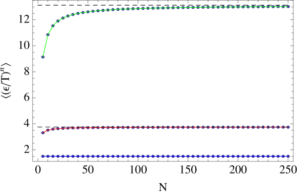
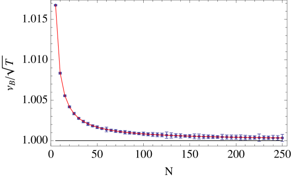
Figure 3: (Top) Energy moments, $\langle(\epsilon/T)^{n}\rangle$, for $n=1,2,3$, for values of $N$ up to $N=250$. The blue dots are the results of numerical computations of these quantities, using the scheme described above, and the solid lines correspond to their theoretical values derived in equation (28). The dashed line correspond to the canonical expectations (26). (Bottom) Micro-canonical energy exchange frequency vs. $N$. The blue dots are the results of numerical computations of the energy exchange frequency for the corresponding value of $N$. The solid red line is the numerical integration of the equation (78).

The computation of the mean-squared displacement of the Helfand moment, $H(t)=\sum_{a=1}^{N}a\epsilon_{a}(t)$, yields the conductivity in the limit of large system sizes,

$$\kappa=\lim_{N\to\infty}\frac{1}{N(E/N)^{2}}\lim_{n\to\infty}\bigg{\langle}\frac{1}{2\tau_{n}}\Delta H(\tau_{n})^{2}\bigg{\rangle}_{E/N}\,.$$ (100)

As seen in figure 4, the conductivity is identical to the collision frequency, in accordance with equation (5):

$$\frac{\kappa}{\nu_{\mathrm{B}}}=\left\{\begin{array}[]{l@{\quad}l}0.9994\pm 0.0016\,,&(1D)\,,\\ 0.9993\pm 0.0026\,,&(2D)\,.\end{array}\right.$$ (101)

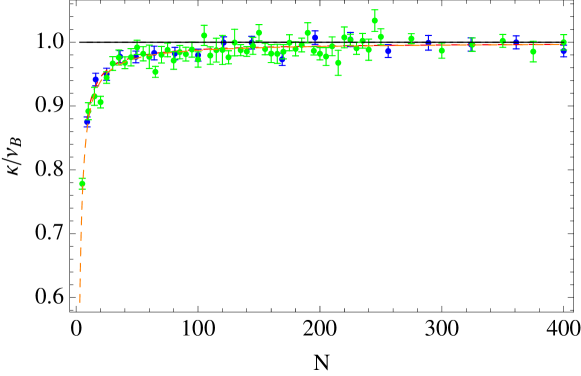
Figure 4: Ratio between the mean squared displacement of the Helfand moment and energy exchange frequency for one- (green) and two-dimensional (blue) lattices of cells vs. the size of the lattices $N$. The ratio $\kappa/\nu_{\mathrm{B}}$ is the infinite $N$ extrapolation of these data, which we evaluate by linear regression (dashed red line). Fitting the data points corresponding to $N\geq 9$ (of which only a fraction are displayed here) with weights inversely proportional to the sizes of their error bars, we obtain, for the one-dimensional lattice, $\kappa/\nu_{\mathrm{B}}=0.9994\pm 0.0016$, with $N$ up to 400, and, for the two-dimensional lattice, $\kappa/\nu_{\mathrm{B}}=0.9993\pm 0.0026$, with $N$ up to $400$ ($=20\times 20$).

7.2 Non-equilibrium simulation

Non-equilibrium boundary conditions are easily implemented on one-dimensional lattices by thermalising the boundary cells at respective temperatures $T_{-}=0.5$ and $T_{+}=1.5$ according to the scheme detailed in [6].

The heat conductivity is evaluated by computing the stationary heat current, $J_{\mathrm{H}}$, and comparing it to the temperature gradient according to

$$J_{\mathrm{H}}=-\kappa\frac{T_{+}-T_{-}}{N}\,,$$ (102)

in the limit of large system sizes $N$.

Denoting by $P^{(2)}_{a,a+1}(\epsilon,\epsilon^{\prime})$ the two-point marginal of the stationary state associated with cells $a$ and $a+1$ at respective energies $\epsilon$ and $\epsilon^{\prime}$, the heat current is

$$J_{\mathrm{H}}\equiv\int\/\mathrm{d}\/\epsilon\/\mathrm{d}\/\epsilon^{\prime}j(\epsilon,\epsilon^{\prime})P^{(2)}_{a,a+1}(\epsilon,\epsilon^{\prime})\,.$$ (103)

A numerical computation of this quantity was performed for different system sizes, as shown on the left panel of figure 5. The result of the infinite $N$ extrapolation yields

$$\frac{\kappa}{\nu_{\mathrm{B}}}=1.00016\pm 0.0005\,.$$ (104)

According to Fourier’s law, the corresponding local temperature profile is expected to be

$$T_{n}=\left[\frac{1}{2}(T_{-}^{\frac{3}{2}}+T_{+}^{\frac{3}{2}})+\frac{n}{N+1}(T_{+}^{\frac{3}{2}}-T_{-}^{\frac{3}{2}})\right]^{\frac{2}{3}}\,,$$ (105)

which is confirmed numerically as seen in the right panel of figure 5.

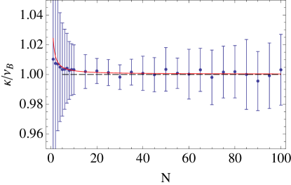
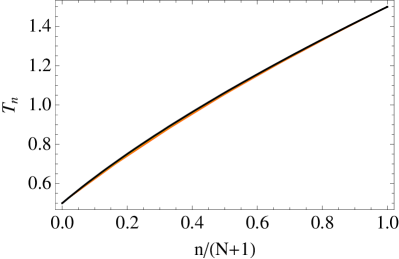
Figure 5: (Left) Ratio between the heat current (103) and local temperature gradient under thermal boundary conditions at the temperatures $T_{+}=1.5$ and $T_{-}=0.5$, corresponding to the temperature profiles shown above. The system sizes $N$ here range from $N=1$ to $N=100$. The ratio $\kappa/\nu_{\mathrm{B}}$ is computed from the infinite $N$ extrapolation of these data, evaluated by linear regression with respect to $1/N$ (solid red line). Fitting the data points weighed according to the sizes of their error bars, we obtain $\kappa/\nu_{\mathrm{B}}=1.00016\pm 5\,10^{-4}$. (Right) Temperature profiles obtained in the non-equilibrium stationary states of systems in contact with stochastically thermalised cells at $n=0$ ($T_{-}=1/2$) and $n=N+1$ ($T_{+}=3/2$). The thick black line corresponds to the profile (105) expected from Fourier’s law. Different system sizes are displayed, going from $N=5$ to $N=100$. The data is barely distinguishable from the curve (105) when $N$ is sufficiently large.

8 Conclusions and perspectives

To summarize, we have successfully extended the results presented in [6] to the confining dynamics of rarely interacting hard spheres. Our results thus further validate the claim that the identity between heat conductivity and collision frequency in such systems of confined particles interacting through rare hard core collisions is largely independent of the details of the underlying dynamics.

In a forthcoming publication, we will show that the dimensionality of the underlying dynamics is indeed arbitrary. In particular, one can consider systems which consist of a solid structure of confining pores of arbitrary shapes in which gas particles of arbitrary numbers are trapped. The geometry of the pores must be such that each isolated pore contains a fixed number of hard spheres with micro-canonical equilibrium measure whose energy is the sum of the kinetic energies of the gas particles. Under the assumption that relaxation to this local equilibrium measure takes place on time scales smaller than the time scales of energy exchanges between neighbouring pores, a master equation of the form (1) can be derived to describe the energy exchange process. The corresponding stochastic kernel will in this case depend on the geometry of the pores involved in the energy exchange and, in particular, on the precise number of particles in those pores. The symmetry relations (8) will thus reflect local properties of the system whose overall average yields the corresponding macroscopic properties. In this sense, one expects that Fourier’s law can be derived in a rather general setting for such systems of confined particles, and the value of the heat conductivity expressed in terms of the frequency of energy exchanges between the cells.

References

References

- [1] Bonetto F, Lebowitz J L, and Rey-Bellet L 2000 Fourier Law: A Challenge To Theorists in Fokas A, Grigoryan A, Kibble T, Zegarlinski B (Eds.) Mathematical Physics 2000 (Imperial College, London).
- [2] Gaspard G and Gilbert T 2008 Heat conduction and Fourier’s law by consecutive local mixing and thermalization Phys. Rev. Lett. 101 020601.
- [3] Gilbert T and Lefevere R 2008 Heat conductivity from molecular chaos hypothesis in locally confined billiard systems Phys. Rev. Lett. 101 200601.
- [4] Machta J and Zwanzig R 1983 Diffusion in a Periodic Lorentz Gas Phys. Rev. Lett. 50 1959.
- [5] Gaspard G and Gilbert T 2008 Heat conduction and Fourier’s law in a class of many particle dispersing billiards New J. Phys. 10 103004.
- [6] Gaspard G and Gilbert T 2008 On the derivation of Fourier’s law in stochastic energy exchange systems J. Stat. Mech. (2008) P11021.
- [7] Chernov N and Markarian R 2006 Chaotic billiards Math. Surveys and Monographs 127 (AMS, Providence, RI).
- [8] Ernst M H, Dorfman J R, Hoegy W R, and Van Leeuwen J M J 1969 Hard-sphere dynamics and binary-collision operators Physica 45 127; Dorfman J R and Ernst M H 1989 Hard-sphere binary-collision operators J. Stat. Phys. 57 581.
- [9] Gillespie D T 1976 General Method for Numerically Simulating the Stochastic Time Evolution of Coupled Chemical Reactions J. Comp. Phys. 22 403-434.
- [10] Gillespie D T 1977 Exact Stochastic Simulation of Coupled Chemical Reactions J. Phys. Chem. 81 2340-2361.