Casimir-Lifshitz Interaction between Dielectrics of Arbitrary Geometry: A Dielectric Contrast Perturbation Theory

Abstract

The general theory of electromagnetic–fluctuation–induced interactions in dielectric bodies as formulated by Dzyaloshinskii, Lifshitz, and Pitaevskii is rewritten as a perturbation theory in terms of the spatial contrast in (imaginary) frequency dependent dielectric function. The formulation can be used to calculate the Casimir-Lifshitz forces for dielectric objects of arbitrary geometry, as a perturbative expansion in the dielectric contrast, and could thus complement the existing theories that use perturbation in geometrical features. We find that expansion in dielectric contrast recasts the resulting Lifshitz energy into a sum of the different many-body contributions. The limit of validity and convergence properties of the perturbation theory is discussed using the example of parallel semi-infinite objects for which the exact result is known.

I Introduction

Macroscopic material boundaries that interact with fluctuating electromagnetic fields experience an induced interaction amongst themselves. This was first demonstrated for the case of two perfectly conducting parallel plates by Casimir Casimir48 , and was subsequently generalized to take into account frequency dependent dielectric properties of the objects by Lifshitz Lifshitz . Relevant experimental studies were being developed for a long time old until recently several high precision measurements of the Casimir force were performed measure . Lifshitz theory and its application to various situations such as materials with finite conductivity and finite temperature effects has been an active area of research in the past few years klim

The recent trend in miniaturization of mechanical devices naturally brought up the issue that Casimir-Lifshitz interactions need to be taken into consideration when small components are at close proximity of each other nanomech . For traditional design strategies these forces, which could dominate all the others at distances smaller than a few hundred nanometers, are to be eliminated. On the other hand, one can also imagine using them for novel design ideas that could potentially change the way we think about designing mechanical systems at that scale machine . For these reasons, it is necessary to develop a better understanding of Casimir-Lifshitz interactions when the objects involved do not have ideal geometrical shapes.

This is far from a trivial task, but in recent years there have been a number of significant developments to this end. These include perturbative approaches for geometries that can be considered as slightly deformed as compared to some ideal geometries GK ; EHGK ; lambrecht , semiclassical approaches semiclass and classical ray optics approximations Jaffe , multiple scattering and multipole expansions balian ; klich ; multipole1 ; multipole2 ; multipole3 , world-line method gies and exact numerical diagonalization method Emig-exact , and the recently developed numerical Green’s function calculation method Johnson . These different and complementary approaches are useful in understanding the subtleties involved in the dependence of the Casimir-Lifshitz energy on geometrical features of the boundaries.

An interesting result of the Lifshitz theory is that the interaction at small separations are effectively determined by the value of dielectric constants at relatively high (imaginary) frequencies where it is not much different from unity Lifshitz . This suggests that a useful complementary strategy could be pursued based on expansion in dielectric contrast. This approach, which has been the subject of a few recent studies barton ; ramin ; buhmann ; rudi ; milton , is useful as it can treat the effect of the geometry of boundaries exactly. Here we present a systematic formulation of this approach for the calculation of Casimir-Lifshitz energy for dielectric objects of arbitrary shape, in the form of an expansion in powers of the dielectric contrast in the medium (see Fig. 1). We find that expansion in powers of the difference between dielectric constant as compared to the background takes on the form of an expansion in multi-body contributions to the interaction. We provide explicit expressions for each term in the expansion in the form of convolutions of a tensorial kernel. We show that a resummation of the expansion can help augment the convergence properties of the series, and make it applicable to a wider range of dielectric properties.

The rest of the paper is organized as follows. Section II lays out the general formalism used for calculating the Casimir-Lifshitz interaction, which is applicable in general to metals and dielectrics. In Sec. III, the dielectric contrast perturbation theory is developed based on the formalism of Sec. II and an explicit expression is obtained for each term in the expansion. In Sec. IV, the series obtained in Sec. III is resummed using a decomposition of the kernel involved in the general expression for the energy. Section V gives the derivation of the Casimir-Polder energy using the formalism developed in Sec. IV, as an example. The convergence properties of the series obtained as well as the nature of the divergent contributions in the theory are discussed in Sec. VI. Section VII is devoted to a specific class of geometries where two nearly parallel semi-infinite dielectric objects are placed in front of each other. Finally, Sec. VIII concludes the paper with some discussions.

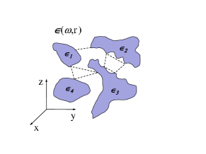
Figure 1: Schematics of the dielectric function profile, and the many-body contributions to the electromagnetic–fluctuation forces.

II General Formalism

Let us assume that we have an assortment of dielectric objects in space with arbitrary shapes and frequency dependent dielectric properties, as sketched in Fig. 1. This medium can be described using a frequency- and space-dependent dielectric function $\epsilon(\omega,{\bf r})$. We consider fluctuating electromagnetic fields in this medium, which we choose to describe in the temporal gauge, where the electrostatic potential vanishes identically, namely $\phi=0$.

We start from the thermal (finite temperature) Green’s function of the electromagnetic field ${\cal D}_{ij}(\zeta_{s};{\bf r},{\bf r}^{\prime})$ in imaginary frequency, where $\zeta_{s}=2\pi sk_{\rm B}T/\hbar$ is the Matsubara frequency with $k_{\rm B}T$ being the thermal energy and $s$ a positive integer LanLif . In the medium described above, the thermal Green function is the solution to the following equation

$$\left[\frac{\zeta_{s}^{2}}{c^{2}}\epsilon(i\zeta_{s},{\bf r})\delta_{ij}+\partial_{i}\partial_{j}-\partial_{l}^{2}\delta_{ij}\right]{\cal D}_{jk}(\zeta_{s};{\bf r},{\bf r}^{\prime})=\delta_{ik}\delta^{3}({\bf r}-{\bf r}^{\prime}).$$ (1)

By introducing the operator

$${\cal K}_{ij}(\zeta_{s};{\bf r},{\bf r}^{\prime})=\left[\frac{\zeta_{s}^{2}}{c^{2}}\epsilon(i\zeta_{s},{\bf r})\delta_{ij}+\partial_{i}\partial_{j}-\partial_{l}^{2}\delta_{ij}\right]\delta^{3}({\bf r}-{\bf r}^{\prime}),$$ (2)

we can write Eq. (1) as

$$\int d^{3}{\bf r}_{1}\;{\cal K}_{ij}(\zeta_{s};{\bf r},{\bf r}_{1}){\cal D}_{jk}(\zeta_{s};{\bf r}_{1},{\bf r}^{\prime})=\delta_{ik}\delta^{3}({\bf r}-{\bf r}^{\prime}),$$ (3)

which means that as an operator we have

$${\cal K}_{ij}(\zeta_{s};{\bf r},{\bf r}^{\prime})={\cal D}_{ij}^{-1}(\zeta_{s};{\bf r},{\bf r}^{\prime}).$$ (4)

Now imagine a process in which we start from the empty space and introduce the dielectric objects into the space in a perturbative manner, similar to the charging process of a capacitor or constructing a charge distribution by bringing infinitesimal charge elements from infinity to assemble the distribution. Using standard diagrammatic techniques Dzy , we can show that the introduction of the dielectric objects causes the Helmholtz free energy of the system to change according to the following formula LanLif

$$\delta{\cal F}=\delta{\cal F}_{0}+k_{\rm B}T{\sum_{s=0}^{\infty}}^{\prime}\int d^{3}{\bf r}_{1}d^{3}{\bf r}_{2}\;{\cal D}_{ij}(\zeta_{s};{\bf r}_{1},{\bf r}_{2})\delta{\cal P}_{ji}(\zeta_{s};{\bf r}_{2},{\bf r}_{1}),$$ (5)

where

$$\delta{\cal P}_{ij}(\zeta_{s};{\bf r},{\bf r}^{\prime})=\frac{\zeta_{s}^{2}}{c^{2}}\delta_{ij}\delta^{3}({\bf r}-{\bf r}^{\prime})\delta\epsilon(i\zeta_{s},{\bf r}),$$ (6)

is the Polarization operator, and the primed summation means that the $s=0$ term has an extra factor of $\frac{1}{2}$. In the diagrammatics, the Polarization operator is formally related to the Green function via the Dyson equation

$${\cal D}_{ij}(\zeta_{s};{\bf r},{\bf r}^{\prime})={\cal D}_{ij}^{(0)}(\zeta_{s};{\bf r},{\bf r}^{\prime})-\int d^{3}{\bf r}_{1}d^{3}{\bf r}_{2}\;{\cal D}_{ik}^{(0)}(\zeta_{s};{\bf r},{\bf r}_{1})\delta{\cal P}_{kl}(\zeta_{s};{\bf r}_{1},{\bf r}_{2}){\cal D}_{lj}(\zeta_{s};{\bf r}_{2},{\bf r}^{\prime}),$$ (7)

where ${\cal D}_{ij}^{(0)}(\zeta_{s};{\bf r},{\bf r}^{\prime})$ denotes the Green function before the change in the dielectric profile due to the introduction of new material. Equation (7) can be solved to yield

$${\cal D}_{ij}^{-1}(\zeta_{s};{\bf r},{\bf r}^{\prime})={{\cal D}_{ij}^{(0)}}^{-1}(\zeta_{s};{\bf r},{\bf r}^{\prime})+\delta{\cal P}_{ij}(\zeta_{s};{\bf r},{\bf r}^{\prime}).$$ (8)

Equations (2) and (6) lead us to the following observation

$$\delta{\cal P}_{ij}(\zeta_{s};{\bf r},{\bf r}^{\prime})=\delta{\cal K}_{ij}(\zeta_{s};{\bf r},{\bf r}^{\prime}).$$ (9)

which helps us to write Eq. (5) in the form of

$$\delta{\cal F}=\delta{\cal F}_{0}+k_{\rm B}T{\sum_{s=0}^{\infty}}^{\prime}{\rm tr}\left[{\cal K}^{-1}\delta{\cal K}\right].$$ (10)

Equation (10) can be formally integrated to yield the following expression for the contribution to the Helmholtz free energy due to Casimir-Lifshitz (CL) interactions:

$${\cal F}_{\rm CL}=k_{\rm B}T{\sum_{s=0}^{\infty}}^{\prime}{\rm tr}\ln\left[{\cal K}_{ij}(\zeta_{s};{\bf r},{\bf r}^{\prime})\right].$$ (11)

At (effectively) low temperatures, we can convert the summation over $s$ into an integration by changing $\Delta s=1$ into $ds=\hbar d\zeta/(2\pi k_{\rm B}T)$. In this case, we find the Casimir-Lifshitz energy as

$$E_{\rm CL}=\hbar\int_{0}^{\infty}\frac{d\zeta}{2\pi}\;{\rm tr}\ln\left[{\cal K}_{ij}(\zeta;{\bf r},{\bf r}^{\prime})\right].$$ (12)

This could be a relatively simple starting point for the calculation of the Casimir-Lifshitz energy in any system.

III Dielectric Contrast Perturbation Theory

We can now construct a systematic perturbation theory scheme based on the above definition of the Casimir-Lifshitz energy. The starting point is to write the dielectric function profile as

$$\epsilon(i\zeta,{\bf r})=1+\delta\epsilon(i\zeta,{\bf r}),$$ (13)

which can be used to decompose the kernel ${\cal K}_{ij}$ into a part that corresponds to the empty space and a perturbation that entails the dielectric inhomogeneity profile. In Fourier space, this reads

$${\cal K}_{ij}(\zeta;{\bf q},{\bf q}^{\prime})={\cal K}_{0,ij}(\zeta,{\bf q})(2\pi)^{3}\delta^{3}({\bf q}+{\bf q}^{\prime})+\delta{\cal K}_{ij}(\zeta;{\bf q},{\bf q}^{\prime}),$$ (14)

where

$${\cal K}_{0,ij}(\zeta,{\bf q})=\frac{\zeta^{2}}{c^{2}}\delta_{ij}+q^{2}\delta_{ij}-q_{i}q_{j},$$ (15)

and

$$\delta{\cal K}_{ij}(\zeta;{\bf q},{\bf q}^{\prime})=\frac{\zeta^{2}}{c^{2}}\delta_{ij}\delta\tilde{\epsilon}(i\zeta,{\bf q}+{\bf q}^{\prime}).$$ (16)

This decomposition can now be used to construct the perturbation theory.

The expressions for the Casimir-Lifshitz energy [Eqs. (11) and (12)] involve ${\rm tr}\ln\left[{\cal K}\right]$, which can be written as a perturbative series by using

$${\rm tr}\ln\left[{\cal K}\right] = {\rm tr}\ln\left[{\cal K}_{0}\right]+{\rm tr}\ln[{\cal I}+{\cal K}_{0}^{-1}\delta{\cal K}]$$

$$= {\rm tr}\ln\left[{\cal K}_{0}\right]+\sum_{n=1}^{\infty}\frac{(-1)^{n-1}}{n}\;{\rm tr}\left[\left({\cal K}_{0}^{-1}\delta{\cal K}\right)^{n}\right],$$

where ${\cal I}$ is the identity tensor and

$${\cal K}_{0,ij}^{-1}(\zeta,{\bf q})=\frac{\frac{\zeta^{2}}{c^{2}}\delta_{ij}+q_{i}q_{j}}{\frac{\zeta^{2}}{c^{2}}\left[\frac{\zeta^{2}}{c^{2}}+q^{2}\right]}.$$ (18)

Putting in the explicit forms for ${\cal K}_{0}^{-1}$ and $\delta{\cal K}$, we can write the explicit form for the trace as

$${\rm tr}[({\cal K}_{0}^{-1}\delta{\cal K})^{n}]=\int\frac{d^{3}{\bf q}^{(1)}}{(2\pi)^{3}}\cdots\frac{d^{3}{\bf q}^{(n)}}{(2\pi)^{3}}\frac{[\frac{\zeta^{2}}{c^{2}}\delta_{i_{1}i_{2}}+q_{i_{1}}^{(1)}q_{i_{2}}^{(1)}]\cdots[\frac{\zeta^{2}}{c^{2}}\delta_{i_{n}i_{1}}+q_{i_{n}}^{(n)}q_{i_{1}}^{(n)}]}{[\frac{\zeta^{2}}{c^{2}}+q^{(1)2}]\cdots[\frac{\zeta^{2}}{c^{2}}+q^{(n)2}]}\delta\tilde{\epsilon}(i\zeta,-{\bf q}^{(1)}+{\bf q}^{(2)})\cdots\;\delta\tilde{\epsilon}(i\zeta,-{\bf q}^{(n)}+{\bf q}^{(1)}).$$ (19)

The above expression contains the geometric information about the arrangement of the dielectric objects through the Fourier transform of the dielectric function profile. We can now rewrite Eq. (19) in real space, and find the following series expression for the Casimir-Lifshitz energy of any heterogeneous dielectric medium

$$E_{\rm CL}=\hbar\int_{0}^{\infty}\frac{d\zeta}{2\pi}\;\sum_{n=1}^{\infty}\frac{(-1)^{n-1}}{n}\;\int d^{3}{\bf r}_{1}\cdots d^{3}{\bf r}_{n}\;{\cal G}^{\zeta}_{i_{1}i_{2}}({\bf r}_{1}-{\bf r}_{2})\cdots\;{\cal G}^{\zeta}_{i_{n}i_{1}}({\bf r}_{n}-{\bf r}_{1})\;\delta\epsilon(i\zeta,{\bf r}_{1})\cdots\;\delta\epsilon(i\zeta,{\bf r}_{n}),$$ (20)

where the Green function defined as ${\cal G}^{\zeta}_{ij}({\bf r})=\frac{\zeta^{2}}{c^{2}}{\cal K}_{0,ij}^{-1}(\zeta,{\bf r})$ reads

$${\cal G}^{\zeta}_{ij}({\bf r})=\frac{\zeta^{2}}{c^{2}}\frac{{\rm e}^{-\zeta r/c}}{4\pi r}\left[\delta_{ij}\left(1+\frac{c}{\zeta r}+\frac{c^{2}}{\zeta^{2}r^{2}}\right)-\frac{r_{i}r_{j}}{r^{2}}\left(1+3\frac{c}{\zeta r}+3\frac{c^{2}}{\zeta^{2}r^{2}}\right)\right]+\frac{1}{3}\delta_{ij}\delta^{3}({\bf r}),$$ (21)

in real space. The tensorial kernel ${\cal G}^{\zeta}_{ij}$, has the structure of the electric field of a radiating dipole in imaginary frequency, including the delta function contribution that ensures appropriate behavior of the expression in the near-field Jackson . This kernel has been introduced some time ago in connection with van der Waals interactions Green .

The main result of Eq. (20) [and a re-summed version of it given in Eq. (29) below] has a number of interesting characteristics. First, We find that an expansion in powers of $\delta\epsilon$ automatically turns into a summation of integrated contributions of $n$-body interactions. Moreover, all of the $n$-body interaction terms have simple explicit expressions in terms of a single fundamental kernel that mediates the two-body part of the interaction. Finally, we find a closed form expression for the Lifshitz energy for any geometrical arrangement of dielectric bodies in terms of quadratures, which is amenable to simple diagrammatic rules and can hence be easily adapted for numerical computations at any given order of the perturbation theory.

IV Clausius-Mossotti Resummation of the Perturbation Theory

The perturbation theory developed above uses the spatial contrast in the dielectric function as expansion parameter and this in general may not be a suitably controlled expansion parameter, especially at zero frequency where the dielectric contrast could be considerably larger than unity (see Sec. VI for more discussion). The formulation can be augmented by resumming the perturbation theory such that it is organized as an expansion in powers of the combination $\frac{\delta\epsilon}{1+\delta\epsilon/3}=\frac{3(\epsilon-1)}{(2+\epsilon)}$ instead of $\delta\epsilon$. The new expansion parameter, which reminds us of the Clausius-Mossotti equation for molecular polarizability Jackson , is systematically smaller than the dielectric contrast itself, and is finite even for real metals at zero frequency (where the dielectric contrast diverges).

The key to this remedy lies in the Dirac delta function term in the expression of the kernel in Eq. (21). This suggests a decomposition of the form

$${\cal K}_{0}^{-1}=\frac{c^{2}}{3\zeta^{2}}\left[3{\cal A}+{\cal I}\right],$$ (22)

to be used in the formulation, where the operator ${\cal A}$ is defined as

$${\cal A}_{ij}(\zeta,{\bf q})=\frac{2\frac{\zeta^{2}}{c^{2}}\delta_{ij}+3q_{i}q_{j}-q^{2}\delta_{ij}}{3\left[\frac{\zeta^{2}}{c^{2}}+q^{2}\right]},$$ (23)

in Fourier space, and as

$${\cal A}_{ij}(\zeta,{\bf r}) = \frac{\zeta^{2}}{c^{2}}\frac{{\rm e}^{-\zeta r/c}}{4\pi r}\left[\delta_{ij}\left(1+\frac{c}{\zeta r}+\frac{c^{2}}{\zeta^{2}r^{2}}\right)\right.$$ (24)

$$\left.-\frac{r_{i}r_{j}}{r^{2}}\left(1+3\frac{c}{\zeta r}+3\frac{c^{2}}{\zeta^{2}r^{2}}\right)\right],$$

in position space. Putting Eq. (22) in Eq. (LABEL:eq:trlnK), we find

$${\rm tr}\ln\left[{\cal K}\right] = {\rm tr}\ln\left[{\cal K}_{0}\right]+{\rm tr}\ln\left[{\cal I}+{\cal K}_{0}^{-1}\delta{\cal K}\right],$$ (25)

$$= {\rm tr}\ln\left[{\cal K}_{0}\right]+{\rm tr}\ln\left[\left({\cal I}+\frac{c^{2}}{3\zeta^{2}}{\cal I}\delta{\cal K}\right)+\frac{c^{2}}{\zeta^{2}}{\cal A}\delta{\cal K}\right],$$

$$= {\rm tr}\ln\left[{\cal K}_{0}\right]+{\rm tr}\ln\left[{\cal I}+\frac{c^{2}}{3\zeta^{2}}\delta{\cal K}\right]$$

$$+{\rm tr}\ln\left[{\cal I}+\frac{c^{2}}{\zeta^{2}}{\cal A}\delta{\cal K}\left({\cal I}+\frac{c^{2}}{3\zeta^{2}}\delta{\cal K}\right)^{-1}\right].$$

Defining a new operator

$$\delta{\cal B}\equiv\frac{c^{2}}{\zeta^{2}}\delta{\cal K}\left({\cal I}+\frac{c^{2}}{3\zeta^{2}}\delta{\cal K}\right)^{-1},$$ (26)

which in position space has the following explicit form

$$\delta{\cal B}_{ij}(\zeta;{\bf r},{\bf r}^{\prime})=\left[\frac{\delta\epsilon(i\zeta,{\bf r})}{1+\frac{1}{3}\delta\epsilon(i\zeta,{\bf r})}\right]\delta_{ij}\delta^{3}({\bf r}-{\bf r}^{\prime}),$$ (27)

we can rewrite Eq. (25) as

$${\rm tr}\ln\left[{\cal K}\right] = {\rm tr}\ln\left[{\cal K}_{0}\right]+{\rm tr}\ln\left[{\cal I}+\frac{c^{2}}{3\zeta^{2}}\delta{\cal K}\right]+{\rm tr}\ln\left[{\cal I}+{\cal A}\delta{\cal B}\right],$$ (28)

$$= {\rm tr}\ln\left[{\cal K}_{0}\right]+{\rm tr}\ln\left[{\cal I}+\frac{c^{2}}{3\zeta^{2}}\delta{\cal K}\right]$$

$$+\sum_{n=1}^{\infty}\frac{(-1)^{n-1}}{n}\;{\rm tr}\left[\left({\cal A}\delta{\cal B}\right)^{n}\right].$$

This form can now be used to recast the perturbative expansion for the Casimir-Lifshitz energy as a systematic expansion in powers of the new perturbation parameter, which is always less than unity. We thus find

$$E_{\rm CL} = \hbar\int_{0}^{\infty}\frac{d\zeta}{2\pi}\;\sum_{n=1}^{\infty}\frac{(-1)^{n-1}}{n}\int d^{3}{\bf r}_{1}\cdots d^{3}{\bf r}_{n}$$ (29)

$$\times {\cal A}_{i_{1}i_{2}}({\bf r}_{1}-{\bf r}_{2})\cdots{\cal A}_{i_{n}i_{1}}({\bf r}_{n}-{\bf r}_{1})$$

$$\times \left[\frac{\delta\epsilon(i\zeta,{\bf r}_{1})}{1+\frac{1}{3}\delta\epsilon(i\zeta,{\bf r}_{1})}\right]\cdots\left[\frac{\delta\epsilon(i\zeta,{\bf r}_{n})}{1+\frac{1}{3}\delta\epsilon(i\zeta,{\bf r}_{n})}\right],$$

in real space. In this result, we have neglected two remaining terms in Eq. (28). The first one is the trivial term ${\rm tr}\ln\left[{\cal K}_{0}\right]$ that corresponds to the self energy of vacuum and could be easily eliminated as it does not depend on any of the physical parameters involved. The second term in Eq. (28) is a singular contribution, which has the explicit form of

$$\hbar\int_{0}^{\infty}\frac{d\zeta}{2\pi}\int d^{3}{\bf r}\;\ln\left[1+\frac{1}{3}\delta\epsilon(i\zeta,{\bf r})\right]\int\frac{d^{3}{\bf q}}{(2\pi)^{3}}.$$ (30)

This term does depend on the geometry of the dielectric objects, and need to be subtracted off for any given geometry and dielectric configuration. We will comment on the general issues related to such divergent contributions as well as the convergence properties of the series in the following Section.

V Example: Casimir-Polder Interaction

To see how the formalism works, let us use it to calculate the Casimir-Polder (CP) interaction between two objects at long separations. Consider a sphere of volume $v_{1}$ and dielectric function $\epsilon_{1}(i\zeta)$ located at the origin, and a sphere of volume $v_{2}$ and dielectric function $\epsilon_{2}(i\zeta)$ located at a separation $R$ from the first one. To calculate the Casimir-Polder energy, we can use Eq. (29) in conjunction with

$$\frac{\delta\epsilon(i\zeta,{\bf r})}{1+\frac{1}{3}\delta\epsilon(i\zeta,{\bf r})} = \frac{\delta\epsilon_{1}(i\zeta)}{1+\frac{1}{3}\delta\epsilon_{1}(i\zeta)}~{}v_{1}\delta^{3}({\bf r})$$ (31)

$$+ \frac{\delta\epsilon_{2}(i\zeta)}{1+\frac{1}{3}\delta\epsilon_{2}(i\zeta)}~{}v_{2}\delta^{3}({\bf r}-{\bf R}).$$

This is a singular form for the profile and is only valid in the limit that the separation is much larger than the typical size of the objects. Therefore, to be consistent with this singular limit we should only keep the leading order term in the size of the objects. A typical term in Eq. (29) with this dielectric profile, which does not contribute to the self energies of the two objects, would (symbolically) look like

$$\left(\frac{\delta\epsilon_{1}(i\zeta)}{1+\frac{1}{3}\delta\epsilon_{1}(i\zeta)}\right)^{m}~{}v_{1}^{m}\left(\frac{\delta\epsilon_{2}(i\zeta)}{1+\frac{1}{3}\delta\epsilon_{2}(i\zeta)}\right)^{n-m}~{}v_{2}^{n-m}$$

$$\times~{}{\cal A}_{i_{1}i_{2}}({\bf 0}_{1})\cdots{\cal A}_{i_{m}i_{m+1}}(-{\bf R}){\cal A}_{i_{m+1}i_{m+2}}({\bf 0}_{2})\cdots{\cal A}_{i_{n}i_{1}}({\bf R}),$$

(32)

which involves multiple powers of the quantity

$$f=v~{}{\cal A}_{ij}({\bf 0}).$$ (33)

Using the proper definition of $f$ within our singular description of the objects, we find

$$f=\lim_{{\bf r}\to{\bf 0}}~{}\left[\left(\frac{4\pi}{3}r^{3}\right){\cal A}_{ij}({\bf r})\right]=0.$$ (34)

Therefore, to the leading order, we find

$$E_{\rm CP} = -\hbar\int_{0}^{\infty}\frac{d\zeta}{2\pi}~{}\left[\frac{v_{1}\delta\epsilon_{1}(i\zeta)}{1+\frac{1}{3}\delta\epsilon_{1}(i\zeta)}\right]\left[\frac{v_{2}\delta\epsilon_{2}(i\zeta)}{1+\frac{1}{3}\delta\epsilon_{2}(i\zeta)}\right]$$ (35)

$$\times~{}{\cal A}_{ij}({\bf R}){\cal A}_{ji}(-{\bf R}).$$

Using the following definition for dynamic polarizability

$$\alpha(i\zeta)=\frac{1}{4\pi}\left[\frac{v_{1}\delta\epsilon_{1}(i\zeta)}{1+\frac{1}{3}\delta\epsilon_{1}(i\zeta)}\right],$$ (36)

and Eq. (24), we can rewrite Eq. (35) as

$$E_{\rm CP} = -\frac{\hbar}{\pi R^{6}}\int_{0}^{\infty}d\zeta~{}\alpha_{1}(i\zeta)\alpha_{2}(i\zeta)~{}{\rm e}^{-2\zeta R/c}$$ (37)

$$\times \left[3+6\frac{\zeta R}{c}+5\frac{\zeta^{2}R^{2}}{c^{2}}+2\frac{\zeta^{3}R^{3}}{c^{3}}+\frac{\zeta^{4}R^{4}}{c^{4}}\right].$$

Ignoring the frequency dependence of the polarizabilities, we find

$$E_{\rm CP}=-\frac{23}{4\pi}\frac{\hbar c}{R^{7}}\alpha_{1}\alpha_{2},$$ (38)

which is the celebrated result for Casimir-Polder interaction CP . The above results could also be obtained using Eq. (20) in which case the corresponding $f$-factors would create nonvanishing constant values that would need to be added up to generate the Clausius-Mossotti form of the polarizabilities.

While the limiting form at longest separations can be obtained by this simple treatment, the correction terms (that are appreciable at closer separations) will systematically be produced from to the $f$-factors that technically speaking correspond to higher multipole contributions to the Casimir-Polder energy, as well as many body contributions. To keep track of these corrections in a systematic way requires a multipole expansion type approach of the type developed in Refs. multipole1 ; multipole2 ; multipole3 . Finally, we note that the simple treatment given above corresponds to spheres where the symmetry of the object easily guarantees that Eq. (34) holds true. For more complicated geometries, the question of orientation as well as the shape of the object complicates matters more multipole1 ; multipole3 and a more systematic approach is needed.

VI Convergence and Regularization of the Perturbation Theory

VI.1 When is the series expansion convergent?

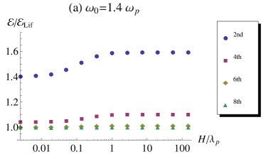
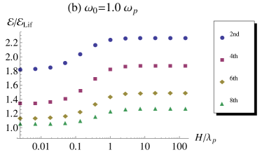
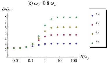
Figure 2: Comparison of the expansion in Eq. (20) up to the 2nd, 4th, 6th, and 8th order, with the exact Lifshitz result for a pair of parallel semi-infinite dielectrics, as a function of their separation $H$ in units of the plasma wavelength $\lambda_{p}$. The dielectric constant of both objects is chosen as Eq. (40) with (a) $\omega_{0}=1.4\;\omega_{p}$, (b) $\omega_{0}=1.0\;\omega_{p}$, and (c) $\omega_{0}=0.8\;\omega_{p}$.

Because the formulation is constructed as a perturbation theory, which can perhaps complement other perturbation theories for Casimir-Lifshitz interaction between objects of arbitrary geometry, we need to address the convergence properties of the expansion. To examine the convergence property of Eq. (20), we can use a specific example for which the exact Casimir-Lifshitz energy is known, and compare it with the perturbative approximations at given orders. We consider the case of two identical semi-infinite dielectric objects with flat boundaries that are placed parallel to each other at a separation $H$. The exact expression for the energy per unit area for this problem is known to be Lifshitz

$${\cal E}_{\rm Lif} = \frac{\hbar}{4\pi^{2}c^{2}}\int_{0}^{\infty}d\zeta\;\zeta^{2}\int_{1}^{\infty}dp\;p$$ (39)

$$+\left\{\ln\left[1-\frac{(s-p)^{2}}{(s+p)^{2}}{\rm e}^{-2p\zeta H/c}\right]\right.$$

$$+\left.\ln\left[1-\frac{(s-p\epsilon)^{2}}{(s+p\epsilon)^{2}}{\rm e}^{-2p\zeta H/c}\right]\right\},$$

where $s=\sqrt{\epsilon-1+p^{2}}$. We assume a simple form of

$$\epsilon(i\zeta)=1+\frac{\omega_{p}^{2}}{\omega_{0}^{2}+\zeta^{2}},$$ (40)

for the dielectric constant (in imaginary frequency), where $\omega_{p}$ represents the plasma frequency, from which the plasma wavelength $\lambda_{p}=2\pi c/\omega_{p}$ can be extracted. We have checked that a dissipative term of the form $\gamma\zeta$ in the denominator of Eq. (40) would not alter are results significantly for realistic values of $\gamma$, therefore we have neglected this term for simplicity of our presentation.

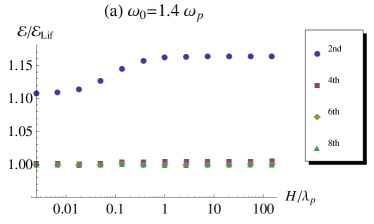
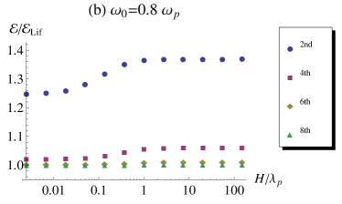
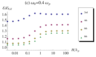
Figure 3: Comparison of the expansion in Eq. (29) (the so-called Clausius-Mossotti resummation) up to the 2nd, 4th, 6th, and 8th order, with the exact Lifshitz result for a pair of parallel semi-infinite dielectrics, as a function of their separation $H$ in units of the plasma wavelength $\lambda_{p}$. The dielectric constant of both objects is chosen as Eq. (40) with (a) $\omega_{0}=1.4\;\omega_{p}$, (b) $\omega_{0}=0.8\;\omega_{p}$, and (c) $\omega_{0}=0.4\;\omega_{p}$.

In Fig. 2, the ratio between the energy as calculated from Eq. (20) and the exact Lifshitz result is shown as a function of the separation, up to the second, fourth, sixth, and eighth order in perturbation theory. The results clearly show a crossover between two asymptotic regimes near $H=\lambda_{p}/(2\pi)$ note1 . Figure 2a corresponds to $\omega_{0}=1.4\;\omega_{p}$ and shows a rapid convergence. This can be understood from the fact that even at zero frequency where the dielectric contrast has its largest value, this example yields $\delta\epsilon(0)=0.5$ that is smaller than unity. Figure 2b shows that when $\omega_{0}=1.0\;\omega_{p}$ the series is still convergent (despite $\delta\epsilon(0)=1$), although not as rapidly as in the example of Fig. 2a. For $\omega_{0}=0.8\;\omega_{p}$, the series is divergent, as Fig. 2c shows. Therefore, the series in Eq. (20) appears to be rapidly convergent when $\delta\epsilon(0)<1$, and the convergence is considerably more efficient for $H<\lambda_{p}/(2\pi)$ [as compared to $H>\lambda_{p}/(2\pi)$], especially for $\delta\epsilon(0)\lesssim 1$.

The resummation of the perturbation theory discussed in Sec. IV improves the convergence property of the series as it effectively replaces $\delta\epsilon$ (that can have any value) by $\frac{\delta\epsilon}{1+\delta\epsilon/3}=\frac{3(\epsilon-1)}{(2+\epsilon)}$, which is bound to be between $0$ and $3$ even for real metals at zero frequency. More explicitly, using Eq. (40) one can see that the expansion parameter at zero frequency, which is the parameter that controls the convergence of the series at large separations, changes from $\delta\epsilon(0)=\omega_{p}^{2}/\omega_{0}^{2}$ to $3\omega_{p}^{2}/(3\omega_{0}^{2}+\omega_{p}^{2})$. This suggests that at large separations, the series [in Eq. (29)] should now be convergent for $\omega_{0}>0.8\;\omega_{p}$ (so that the expansion parameter is smaller than unity). Figure 3 shows the convergence property of a few examples using Eq. (29) instead of Eq. (20). For $\omega_{0}=1.4\;\omega_{p}$, a much more rapid convergence is observed as shown in Fig. 3a, while the previously divergent case of $\omega_{0}=0.8\;\omega_{p}$ now shows a good convergence, as seen in Fig. 3b and in agreement with the argument above. As Fig. 3c shows, even for $\omega_{0}=0.4\;\omega_{p}$ one still observes a good convergence despite the fact that the zero frequency expansion parameter is equal to 2.

Figure 4a shows the result of the expansion for $\omega_{0}=0.3\;\omega_{p}$. Interestingly, it appears that in this case the series is (at least up the eighth order in perturbation) convergent for $H<\lambda_{p}/(2\pi)$, while it clearly diverges for $H>\lambda_{p}/(2\pi)$. One can roughly say that the appropriate parameter that controls the convergence at small separations is the expansion parameter at $\zeta=\omega_{0}$, which is $3\omega_{p}^{2}/(6\omega_{0}^{2}+\omega_{p}^{2})$. For $\omega_{0}=0.3\;\omega_{p}$, this parameter is $\simeq 2$, which is consistent with the value of the zero frequency expansion parameter in the borderline convergence case at large separations obtained for $\omega_{0}=0.4\;\omega_{p}$. Finally, for $\omega_{0}=0.1\;\omega_{p}$, the series is divergent, as can be seen in Fig. 4b. It is interesting that the criterion for convergence seems to be that the relevant expansion parameter—i.e. the parameter at the relevant frequency—needs to be smaller than 2.

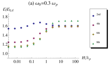
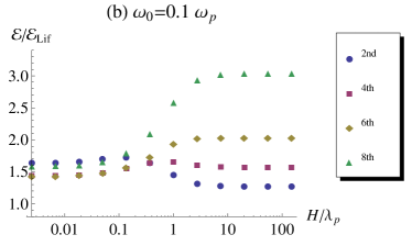
Figure 4: Comparison of the expansion in Eq. (29) (the so-called Clausius-Mossotti resummation) up to the 2nd, 4th, 6th, and 8th order, with the exact Lifshitz result for a pair of parallel semi-infinite dielectrics, as a function of their separation $H$ in units of the plasma wavelength $\lambda_{p}$. The dielectric constant of both objects is chosen as Eq. (40) with (a) $\omega_{0}=0.3\;\omega_{p}$ (corresponding to silicon) and (b) $\omega_{0}=0.1\;\omega_{p}$.

VI.2 Divergencies and Regularization

A general issue with the calculation of the Casimir-Lifshitz energy is the appearance of divergent contributions, like in any quantum field theory calculation. In the case of a system with arbitrary geometry, it is not clear how these divergencies depend on the details of the geometry, so that they could be identified and dealt with in a systematic way. The present formulation also suffers from the presence of divergent terms, but similar to any perturbative field theory with a manifest recipe for constructing each term, these divergent contributions could be systematically identified and regularized order by order in perturbation.

As pointed out by Barton barton , it is important to examine the nature of the divergent contributions, and for example determine whether they are controlled by the minimum possible distance between atoms and molecules (i.e. cutoff on wavevector), transparency of the materials at high frequency (i.e. plasma frequency as cutoff) or ultraviolet frequency cutoff in vacuum. This point has not always been carefully dealt with in the literature of the Casimir-Lifshitz interactions, partly because the largely used perfect conductor limit already blurs this distinction at the outset when it assumes the plasma frequency is infinite.

In our formulation, the divergencies originating from lack of molecular excluded volume in the theory will be regularized using a high wavevector cutoff in the ${\bf q}$ integrals in Eq. (19) or a short distance cutoff in the position integrals in Eqs. (20) and (29). To see how this works let us go to Eq. (19) and look at the ${\bf q}$ integrations. We have

$${\rm tr}[({\cal K}_{0}^{-1}\delta{\cal K})^{n}]=\int\frac{d^{3}{\bf q}^{(1)}}{(2\pi)^{3}} \cdots \frac{d^{3}{\bf q}^{(n)}}{(2\pi)^{3}}~{}M({\bf q}^{(1)},\cdots,{\bf q}^{(n)})$$

$$\times~{}\delta\tilde{\epsilon}(i\zeta,-{\bf q}^{(1)}+{\bf q}^{(2)}) \cdots \delta\tilde{\epsilon}(i\zeta,-{\bf q}^{(n)}+{\bf q}^{(1)}).$$ (41)

where

$$M({\bf q}^{(1)}, \cdots ,{\bf q}^{(n)})=\left[3\zeta^{2n}+\zeta^{2n-2}\left(q^{(1)2}+\cdots+q^{(n)2}\right)\right.$$ (42)

$$\left.+\cdots+\left({\bf q}^{(1)}\cdot{\bf q}^{(2)}\right)\cdots\left({\bf q}^{(n)}\cdot{\bf q}^{(1)}\right)\right]/$$

$$\left[\left(\frac{\zeta^{2}}{c^{2}}+q^{(1)2}\right)\cdots\left(\frac{\zeta^{2}}{c^{2}}+q^{(n)2}\right)\right].$$

Since the (Fourier-space) dielectric contrast profiles only depend on the differences between the wavevectors, we can change the integration variables so that one independent wavevector can be integrated out. Using ${\bf q}_{i}={\bf q}^{(i)}-{\bf Q}$ where ${\bf Q}=\frac{1}{n}({\bf q}^{(1)}+\cdots+{\bf q}^{(n)})$, we find

$${\rm tr}[({\cal K}_{0}^{-1}\delta{\cal K})^{n}]=n\int\frac{d^{3}{\bf q}_{1}}{(2\pi)^{3}} \cdots \frac{d^{3}{\bf q}_{n-1}}{(2\pi)^{3}}\frac{d^{3}{\bf Q}}{(2\pi)^{3}}$$

$$\times~{}M({\bf q}_{1}+{\bf Q}, \cdots ,{\bf q}_{n}+{\bf Q})$$

$$\times~{}\delta\tilde{\epsilon}(i\zeta,-{\bf q}_{1}+{\bf q}_{2}) \cdots \delta\tilde{\epsilon}(i\zeta,-{\bf q}_{n}+{\bf q}_{1}),$$ (43)

where ${\bf q}_{n}=-{\bf q}_{1}-\cdots-{\bf q}_{n-1}$. The integral

$$\int\frac{d^{3}{\bf Q}}{(2\pi)^{3}}~{}M({\bf q}_{1}+{\bf Q},\cdots,{\bf q}_{n}+{\bf Q}),$$

can now be performed independently, and looking at the definition of the kernel $M$ in Eq. (42) we can see that it diverges at high values of ${\bf Q}$ where $M\to 1$. This divergent contribution can be extracted by writing $M=M-1+1$ and separating the $1$ factor, which leads to a regularized contribution proportional to $\int\frac{d^{3}{\bf Q}}{(2\pi)^{3}}=\frac{1}{a^{3}}$. The remaining ${\bf q}$ integrations for this divergent contribution can be carried out, and the series can be summed up to yield an overall singular contribution of the form

$$E_{\rm sing.}=\frac{\hbar}{a^{3}}\int_{0}^{\infty}\frac{d\zeta}{2\pi}\int d^{3}{\bf r}\;\ln\left[\epsilon(i\zeta,{\bf r})\right],$$ (44)

which corresponds to volume terms and can be systematically isolated for any geometry and dielectric configuration. This result entails a similar volume contribution calculated in Ref. barton at the second order in $\delta\epsilon$. Other divergent contributions in the present formulation can be dealt with in a similar manner to the above example.

Finally, we note that using a very similar calculation to the one presented in Sec. V for the Casimir-Polder interaction, one can show that for an arbitrary assortment as depicted in Fig. 1, the Casimir-Lifshitz energy calculated from the present formalism in the limit where the objects are far from each other only contains divergent contributions in the self energies of these objects and all of the terms that depend on the distances—including the many-body terms—are finite.

VII Parallel Semi-Infinite Objects

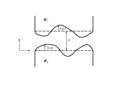
Figure 5: Schematics of two semi-infinite dielectric bodies with boundaries of non-ideal shape.

Due to its importance, we now focus our attention on the specific arrangement shown in Fig. 5, where two nearly parallel semi-infinite dielectric bodies with irregularly shaped boundaries are placed next to each other at a mean separation $H$. We can write down the dielectric function profile in space as

$$\epsilon(i\zeta,{\bf r})=\left\{\begin{array}[]{ll}\epsilon_{2}(i\zeta),&\;H+h_{2}({\bf x})\leq z<+\infty,\\ \\ 1,&\;h_{1}({\bf x})<z<H+h_{2}({\bf x}),\\ \\ \epsilon_{1}(i\zeta),&\;-\infty<z\leq h_{1}({\bf x}),\end{array}\right.$$ (45)

which in Fourier space reads

$$\delta\tilde{\epsilon}(i\zeta,{\bf q}) = \frac{i}{q_{z}}\int d^{2}{\bf x}\;{\rm e}^{i{\bf q}_{\perp}\cdot{\bf x}}$$ (46)

$$\times ~{}\left[\delta\epsilon_{2}\;{\rm e}^{iq_{z}\left[H+h_{2}({\bf x})\right]}-\delta\epsilon_{1}\;{\rm e}^{iq_{z}h_{1}({\bf x})}\right].$$

When the parameters are such that the leading contribution in Eq. (29) comes from the second order term (see Sec. VI), we can simplify the expression for the Casimir-Lifshitz interaction and write it in a closed form that can be readily used in studies of various geometrical effects. A similar strategy has been discussed in Ref. barton , where a large variety of other geometries has been considered. Putting in the dielectric function profile of Eq. (45), we find

$$E_{2} = -\frac{9\hbar}{128\pi^{3}c^{4}}\int_{0}^{\infty}d\zeta\;\zeta^{4}\left[\frac{\epsilon_{1}(i\zeta)-1}{\epsilon_{1}(i\zeta)+2}\right]\left[\frac{\epsilon_{2}(i\zeta)-1}{\epsilon_{2}(i\zeta)+2}\right]$$

$$\times \int d^{2}{\bf x}d^{2}{\bf x}^{\prime}\;{\cal W}\left(\frac{\zeta}{c}[{\bf x}-{\bf x}^{\prime}],\frac{\zeta}{c}[H+h_{2}({\bf x})-h_{1}({\bf x}^{\prime})]\right),$$

(47)

where

$${\cal W}({\bf y},h)=8\;\Gamma\left(0,2\sqrt{y^{2}+h^{2}}\right)+\int_{1}^{\infty}\frac{ds}{s^{3/2}}\;{\rm e}^{-2\sqrt{y^{2}+h^{2}s}}$$

$$\times\left[\frac{3}{(y^{2}+h^{2}s)^{2}}+\frac{6}{(y^{2}+h^{2}s)^{3/2}}+\frac{4\;(1-h^{2}s)}{(y^{2}+h^{2}s)}\right],$$

(48)

and $\Gamma(a,z)=\int_{z}^{\infty}dt\;t^{a-1}\;{\rm e}^{-t}$ is the incomplete gamma function. Note that at this order, the Lifshitz energy is pairwise additive, and that the effect of geometry has been taken into account exactly for any arbitrary profile. In the above result, we have kept the frequency dependence of the dielectric functions as well as the geometry of the boundaries arbitrary for generality of the presentation. The expression in Eq. (47) can be considerably simplified for $h_{1}({\bf x})=0$:

$$\left.E_{2}\right|_{h_{1}({\bf x})=0}=\int d^{2}{\bf x}\;{\cal E}_{2}\left(H+h_{2}({\bf x})\right),$$ (49)

in terms of the original Lifshitz result for the energy per unit area of flat boundaries (within the same scheme of Clausius-Mossotti approximation) Lifshitz

$${\cal E}_{2}(H) = -\frac{9\hbar}{64\pi^{2}c^{2}}\int_{0}^{\infty}d\zeta\;\zeta^{2}\;{\cal L}\left(\frac{\zeta H}{c}\right)$$ (50)

$$\times \left[\frac{\epsilon_{1}(i\zeta)-1}{\epsilon_{1}(i\zeta)+2}\right]\left[\frac{\epsilon_{2}(i\zeta)-1}{\epsilon_{2}(i\zeta)+2}\right],$$

with

$${\cal L}(u)=4(u^{2}-1)E_{1}(2u)+\frac{{\rm e}^{-2u}}{u^{2}}(1+2u+u^{2}-2u^{3}),$$ (51)

and the exponential integral function defined as $E_{n}(z)=\int_{1}^{\infty}dt\;{\rm e}^{-zt}/t^{n}$. This simplification is a general feature that is present for any pairwise additive interactions, as has been shown in Ref. EHGK .

VIII Discussion

When dealing with complicated quantum field theories, it is always helpful to try and formulate complementary perturbative schemes so that the specific point of interest, which is usually out of reach, is approached from different directions. This could potentially provide complementary information that could be compiled to yield an improved insight into the properties of the theory. A good example of this synergy is the perturbation theory and $1/n$ expansion of the $O(n)$ model of the $\phi^{4}$ quantum field theory zinn . A similar strategy has been the underlying motivation for the work presented here: expansion in dielectric contrast allows us to formulate a perturbative scheme for calculating the Casimir-Lifshitz interaction between object with arbitrary geometry keeping the effect of the geometry exact. The motivation behind this alternative approach comes from the fact that at distances smaller than the plasma wavelength the effective dielectric contrast that determines the Casimir-Lifshitz interaction corresponds to the high frequency limit of Eq. (40), which is effectively smaller than the equivalent value for the large distance regime. This view is confirmed by the plots in Figs. 2, 3, and 4, which show that the series expansion in dielectric contrast converges more rapidly at short distances. Interestingly, Fig. 4a suggests that it is possible to have a convergence at distances smaller than the plasma wavelength—typically a few hundred nanometers—while the same series diverges at larger distances. This marginal case is observed for $\omega_{0}=0.3~{}\omega_{p}$, which coincidentally corresponds to silicon silicon that is a common choice for fabrication of small mechanical components with fine geometrical features.

The perturbation theory seems to have good convergence property for materials that have a dielectric contrast of $\sim 2$, or a dielectric constant of $\sim 3$, at the relevant frequency that is zero for large distance asymptotics and $\omega_{0}$ for short distance regime. While this is somewhat restrictive, as for example it does not include real metals, it is not too far from being able to include some commonly used dielectric materials, such as silicon for example. Note that this complementary approach keeps the effect of the geometrical features exact, which is a significant improvement compared with complementary theories that apply to objects with small deformations. Finally, we note that it might be possible to use Borel summation method zinn (or other equivalent techniques) to improve the convergence of the series expansion in the strong coupling limit of dielectric contrast.

In conclusion, we have developed a perturbative scheme for calculating the Casimir-Lifshitz interaction between objects of arbitrary geometry. Explicit expressions are provided for each term in the perturbation theory, as multiple integrals over the bodies of the interacting objects. This method could in principle be used to calculate the interactions at any order using standard numerical integration techniques.

- (1) H.B.G. Casimir, Proc. K. Ned. Akad. Wet. 51, 793 (1948).
- (2) E.M. Lifshitz, Sov. Phys. JETP 2, 73 (1956); I.E. Dzyaloshinskii, E.M. Lifshitz, and L.P. Pitaevskii, Adv. Phys. 10, 165 (1961).
- (3) I.I. Abricossova and B.V. Deryaguin, Dokl. Akad. Nauk. SSSR 90 1055 (1953); M. J. Sparnaay, Physica (Utrecht) 24, 751 (1958); D. Tabor and R.H.S. Winterton, Proc. R. Soc. Lond. A 312, 435 (1969).
- (4) S.K. Lamoreaux, Phys. Rev. Lett. 78, 5 (1997); U. Mohideen and A. Roy, Phys. Rev. Lett. 81, 4549 (1998); A. Roy and U. Mohideen, Phys. Rev. Lett. 82, 4380 (1999); H.B. Chan et al, Science 291, 1941 (2001); F. Chen, U. Mohideen, G.L. Klimchitskaya, and V.M. Mostepanenko, Phys. Rev. Lett. 88, 101801 (2002); Phys. Rev. A 66, 032113 (2002); G. Bressi et al, Phys. Rev. Lett. 88, 041804 (2002); R.S. Decca et al Phys. Rev. Lett. 91, 050402 (2003); D.E. Krause, Phys. Rev. Lett. 98, 050403 (2007); H.B. Chan et al, Phys. Rev. Lett. 101, 030401 (2008).
- (5) For a recent round up of some of the controvercies in this area, see e.g.: G. L. Klimchitskaya, J. Phys.: Conf. Ser. 161 012002 (2009).
- (6) F.M. Serry et al, J. Microelectromech. Syst. 4, 193 (1995); E. Buks and M.L. Roukes, Phys. Rev. B 63, 033402 (2001); H.B. Chan et al, Phys. Rev. Lett. 87, 211801 (2001); G. Palasantzas and J.Th.M. De Hosson, Phys. Rev. B 72, 121409 (R) (2005).
- (7) A. Ashourvan, M.F. Miri, and R. Golestanian, Phys. Rev. Lett. 98, 140801 (2007); Phys. Rev. E 75, 040103 (R) (2007); T. Emig, Phys. Rev. Lett. 98, 160801 (2007); M. Miri and R. Golestanian, Appl. Phys. Lett. 92, 113103 (2008); F.C. Lombardo et al., J. Phys. A 41 164009 (2008); I. Cavero-Peláez et al., Phys. Rev. D 78 065019 (2008).
- (8) R. Golestanian and M. Kardar, Phys. Rev. Lett. 78, 3421 (1997); Phys. Rev. A 58, 1713 (1998); M. Kardar and R. Golestanian, Rev. Mod. Phys. 71, 1233 (1999).
- (9) T. Emig, A. Hanke, R. Golestanian, and M. Kardar, Phys. Rev. Lett. 87, 260402 (2001); Phys. Rev. A 67, 022114 (2003).
- (10) P.A. Maia Neto, A. Lambrecht, and S. Reynaud, Phys. Rev. A 72, 012115 (2005); R.B. Rodrigues, P.A. Maia Neto, A. Lambrecht, and S. Reynaud, Phys. Rev. Lett. 96, 100402 (2006).
- (11) M. Schaden and L. Spruch, Phys. Rev. A 58, 935 (1998).
- (12) R.L. Jaffe and A. Scardicchio, Phys. Rev. Lett. 92, 070402 (2004).
- (13) R. Balian and B. Duplantier, Ann. Phys. (New York) 104, 300 (1977); 112, 165 (1978).
- (14) O. Kenneth and I. Klich, Phys. Rev. Lett. 97, 160401 (2006)
- (15) R. Golestanian, Phys. Rev. E 62, 5242 (2000).
- (16) T. Emig, N. Graham, R.L. Jaffe, and M. Kardar, Phys. Rev. Lett. 99, 170403 (2007).
- (17) T. Emig, N. Graham, R.L. Jaffe, and M. Kardar, Phys. Rev. A 79, 054901 (2009).
- (18) H. Gies and K. Klingmuller, Phys. Rev. Lett. 96, 220401 (2006); Phys. Rev. Lett. 97, 220405 (2006).
- (19) T. Emig, Europhys. Lett. 62, 466 (2003); R. Büscher and T. Emig, Phys. Rev. Lett. 94, 133901 (2005); A. Lambrecht and V.N. Marachevsky, Phys. Rev. Lett. 101, 160403 (2008).
- (20) A. Rodriguez, M. Ibanescu, D. Iannuzzi, F. Capasso, J.D. Joannopoulos, and S.G. Johnson, Phys. Rev. Lett. 99, 080401 (2007); A. Rodriguez, M. Ibanescu, D. Iannuzzi, J.D. Joannopoulos, and S.G. Johnson, Phys. Rev. A 76, 032106 (2007); A. Rodriguez, J.D. Joannopoulos, and S.G. Johnson, Phys. Rev. A 77, 062107 (2008).
- (21) G. Barton, J. Phys. A 34, 4083 (2001).
- (22) R. Golestanian, Phys. Rev. Lett. 95, 230601 (2005).
- (23) S.Y. Buhmann and D.-G. Welsch, Appl. Phys. B 82, 2, 189 (2006).
- (24) G. Veble and R. Podgornik, Eur. Phys. J. E 23, 275 279 (2007).
- (25) K.A. Milton, P. Parashar, and J. Wagner, Phys. Rev. Lett. 101, 160402 (2008).
- (26) E. M. Lifshitz and L. P. Pitaevskii, Statistical Physics: Part 2 (Pergamon, Oxford, 1980).
- (27) A. A. Abrikosov, L. P. Gor’kov, and I. Ye. Dzyaloshinskii, Methods of Quantum Field Theory in Statistical Physics (Dover Publications, New York, 1975).
- (28) J.D. Jackson, Classical Electrodynamics (Wiley, New York, 1999).
- (29) I. Brevik and J.S. Høye, Physica A (Amsterdam) 153, 420 (1988).
- (30) H.B.G. Casimir, and D. Polder, Phys. Rev. 73, 360 (1948).
- (31) Note that the last few data points in Figs. 2, 3, and 4 corresponding to large values of would lie in the thermal regime where the sum over the frequency should be discretized [see Eq. (11)]. These points are presented to help demonstrate the crossover behavior in a convincing way.
- (32) J. Zinn-Justin, Quantum field theory and critical phenomena 2nd edition (Oxford University Press, Oxford, 1993).
- (33) A. Lambrecht, I. Pirozhenko, L. Durafourg, and Ph. Andreucci, Europhys. Lett. 77, 44006 (2007).