Flocking of Multi-agent Dynamical Systems Based on Pseudo-leader Mechanism

Abstract

Flocking behavior of multiple agents can be widely observed in nature such as schooling fish and flocking birds. Recent literature has proposed the possibility that flocking is possible even only a small fraction of agents are informed of the desired position and velocity. However, it is still a challenging problem to determine which agents should be informed or have the ability to detect the desired information. This paper aims to address this problem. By combining the ideas of virtual force and pseudo-leader mechanism, where a pseudo-leader represents an agent who can detect the desired information, we propose a scheme for choosing pseudo-leaders in a multi-agent group. The presented scheme can be applied to a multi-agent group even with an unconnected or switching neighbor graph. Experiments are given to show that the methods presented in this paper are of high accuracy and perform well.

I Introduction

Flocking is a collective behavior of a large group of mobile agents. Typical flocking phenomena include flocks of birds, schools of fish, herds of animals and colonies of bacteria. In nature, animals achieve flocking for various reasons. For example, in order to keep safety in numbers and also to confuse predators, they will form flocks for protection. An agent is more likely to be attacked if it strays away from the flocking group.

As a common demonstration of emergence and emergent behavior, flocking was first simulated on a computer by Craig Reynolds [2]. In 1987, he started with a boid model to build a simulated flock and introduced three rules to simulate flocking:

• Collision Avoidance: steer to avoid collision with nearby flockmates (short range repulsion).

• Velocity Matching: steer to match velocity with nearby flockmates.

• Flock Centering: steer to stay close to nearby flockmates (long range attraction).

The mechanism, known as “separation”, “alignment” and “cohesion”, results in all agents moving in a formation with the same heading and a fixed network structure. From then on, these three rules have been widely used to study flocking behavior.

As a special case of Reynolds’ model, in [3], Vicsek et al. presented a simulation model based on nearest neighborhood law, in which each agent’s heading is updated by the average of the headings of its nearest neighbors and itself. It was shown that the headings of all the group agents converge to a common value.

A lot of works have been published based on Reynolds’ and Vicsek’s models in recent years [4]-[12]. To thoroughly and systematically investigate flocking behavior, artificial potential functions (APFs) are widely used. In [5], Tanner et al. presented an APF in a network with fixed topology which is a differential, nonnegative and radially unbounded function of the distance between two agents. Then, he modified the APF to a nonsmooth one in a network with switching topology which captures the fact that there is no agent interaction beyond a proper distance [6]. Later, Olfati-Saber modified Tanner’s APF and defined another APF which is a bounded and smooth one for switching topology.

In view of the pitfall of regular fragmentation [8], which is a phenomenon of flocking failure most likely occurring for generic set of initial states and large number of agents, Olfati-Saber also introduced a flocking mechanism based on a virtual leader [8]. Even though the initial states is selected randomly, the mechanism can guarantee a flocking behavior. However, this method assumes that all the agents know information about the virtual leader. In consideration of practical use, Shi et al. and Su et al. showed that flocking appears even when only some agents are informed [9]-[11], these we call pseudo-leaders in this paper.

Though Shi et al. and Su et al. showed that flocking could appear when not all the agents are informed in a group, precisely which agents should be informed has not yet been considered. In this paper, we focus on investigating which agents should be selected as pseudo-leaders for flocking in a weighted network. Another difference from previous work is that, in the absence of control, the acceleration of each agent is dynamic. This can be seen in our system model in Section II. That is, if there are no attractive/repulsive control, no information exchange with others and no information received from the virtual leader for an agent, its acceleration is dynamic instead of constant, as is the case in previous work. By using Lyapunov stability theory, a simple criterion for choosing pseudo-leaders is proposed.

The reminder of this paper is organized as follows. In Section II, model depiction, preliminaries about graph theory, and mathematical analysis are briefly introduced. In Section III, the main results are proposed. We investigate how to select pseudo-leaders for flocking in a multi-agent dynamical group with fixed topology. Section IV gives some extensions and discussion of the main results so that one can gain useful insight into the problem of choosing pseudo-leaders. Two computational examples in small-sized and large-scale groups are simulated to illustrate effectiveness of the proposed approach in Section V. We summarize the main ideas and conclusions in Section VI.

II Preliminaries

II-A Graph theory

To make this paper self-contained, some basics of graph theory are recalled [13].

A graph $\mathcal{G}$ is a pair of sets $(\mathcal{V},\mathcal{E})$, where $\mathcal{V}$ is a finite non-empty set of elements called vertices, and $\mathcal{E}$ is a set of unordered pairs of distinct vertices called edges. The set $\mathcal{V}$ and $\mathcal{E}$ are the vertex set and edge set of $\mathcal{G}$, and are often denoted by $\mathcal{V(G)}$ and $\mathcal{E(G)}$, respectively. If $i,j\,\in\,\mathcal{V}$ and $(i,j)\,\in\,\mathcal{E}$, then $i$ and $j$ are adjacent vertices, or neighbors. The set of neighbors of a vertex $i$ is $\mathcal{N}_{i}$. A walk in a graph is a sequence of vertices and edges $j_{0}$, $e_{1}$, $j_{1}$, $\cdots$, $e_{k}$, $j_{k}$, in which each edge $e_{r}\,=\,(j_{r-1},j_{r})$. A path is a walk in which no vertex is repeated. If there is a path between any two vertices of a graph $\mathcal{G}$, then $\mathcal{G}$ is said to be connected. If $\mathcal{G}$ and $\mathcal{G}_{1}$ are graphs with $\mathcal{V}(\mathcal{G}_{1})\,\subseteq\,\mathcal{V(G)}$ and $\mathcal{E}(\mathcal{G}_{1})\,\subseteq\,\mathcal{E(G)}$, then $\mathcal{G}_{1}$ is a subgraph of $\mathcal{G}$.

The position and velocity neighbor graph $\mathcal{G}\,=\,(\mathcal{V},\mathcal{E},\textbf{W})$ is a weighted graph consisting of a set of indexed vertices and a set of ordered edges, where $\textbf{W}\,=\,(w_{ij})\,\in\,\mathbb{R}^{N\,\times\,N}$ is the weight matrix which represents the weighted coupling coefficients of interaction between the agents. If there is a link from vertex $i$ to vertex $j\,(j\,\neq\,i)$, then $w_{ij}\,=\,w_{ji}\,>\,0$ and $w_{ij}$ is the weight; otherwise, $w_{ij}\,=\,0$. Throughout the paper, assume that W is a symmetric matrix satisfying diffusive condition

$$\sum\limits_{j=1}^{N}\,w_{ij}\,=\,0.$$

II-B Model depiction

Consider a multi-agent system consisting of $N$ agents. Here, the moving model of each agent in the group is given by

$$\begin{array}[]{l}\dot{\textbf{p}}_{i}\,=\,\textbf{v}_{i},\\ \dot{\textbf{v}}_{i}\,=\,\textbf{f}(\textbf{v}_{i})\,+\,\textbf{u}_{i},\end{array}$$ (1)

where $1\leq{i}\leq{N}$, $\textbf{p}_{i}\,\in\,\mathbb{R}^{n}$, $\textbf{v}_{i}\,\in\,\mathbb{R}^{n}$ and $\textbf{f}(\textbf{v}_{i})\,\in\,\mathbb{R}^{n}$ denote the position, velocity and the acceleration dynamics (without control input) of the $i$-th agent respectively, and $\textbf{u}_{i}\,\in\,\mathbb{R}^{n}$ is the control input of agent $i$.

The motion model for the virtual leader is

$$\begin{array}[]{l}\dot{\textbf{p}}_{l}\,=\,\textbf{v}_{l},\\ \dot{\textbf{v}}_{l}\,=\,\textbf{f}(\textbf{v}_{l}),\end{array}$$ (2)

where $\textbf{p}_{l}\,\in\,\mathbb{R}^{n}$, $\textbf{v}_{l}\,\in\,\mathbb{R}^{n}$ and $\textbf{f}(\textbf{v}_{l})\,\in\,\mathbb{R}^{n}$ represent the position, velocity and the acceleration dynamics of the virtual leader, respectively.

The flocking task is to design an appropriate control input $\textbf{u}_{i}$ such that Reynolds’ rules are followed, and then all agents moving in a formation with a common heading and collision avoidance.

II-C Mathematical Preliminaries

In this subsection, some useful mathematical definitions, lemmas and assumptions are outlined.

Definition 1. A matrix $\textbf{A}\,=\,(a_{ij})\,\in\,\mathbb{R}^{N\,\times\,N}$ is called reducible if the indices $1,2,\cdots,N$ can be divided into two disjoint nonempty sets $i_{1},i_{2},\cdots,i_{\beta_{1}}$ and $j_{1},j_{2},\cdots,j_{\beta_{2}}$ (with $\beta_{1}\,+\,\beta_{2}\,=\,N$) such that

$$a_{i_{\kappa_{1}},j_{\kappa_{2}}}\,=\,0$$

for $1\,\leq\,\kappa_{1}\,\leq\,\beta_{1}$ and $1\,\leq\,\kappa_{2}\,\leq\,\beta_{2}$. A matrix $\textbf{A}\,=\,(a_{ij})\,\in\,\mathbb{R}^{N\,\times\,N}$ is irreducible if and only if it is not reducible.

A matrix is reducible if and only if it can be placed into block upper-triangular form by simultaneous row/column permutations. In addition, a matrix is reducible if and only if its associated graph is not connected [15].

Definition 2 [14] . A matrix $\textbf{A}\,=\,(a_{ij})\,\in\,\mathbb{R}^{N\,\times\,N}$ is called diagonally dominant if $|a_{ii}|\,\geq\,\,\sum\limits_{j=1,j\,\neq\,i}^{N}\,|a_{ij}|$ for $1\,\leq\,i\,\leq\,N$. A is called strictly diagonally dominant if $|a_{ii}|\,>\,\,\sum\limits_{j=1,j\,\neq\,i}^{N}\,|a_{ij}|$ for $1\,\leq\,i\,\leq\,N$.

The Gershgorin circle theorem [14] results in many interesting conclusions. A strictly diagonally dominant matrix is nonsingular. A symmetric diagonally dominant real matrix with nonnegative diagonal entries is positive semi-definite. If a symmetric matrix is strictly diagonally dominant and all its diagonal elements are positive, then its eigenvalues are positive; if all its diagonal elements are negative, then its eigenvalues are negative. Thus it is obvious that the real part of eigenvalues of the weight matrix W which are all negative except an eigenvalue $0$ with multiplicity one. Throughout the paper, we denote a positive definite (positive semi-definite, negative definite, negative semi-definite) matrix A as $\textbf{A}>\textbf{0}\;(\geq\textbf{0},\;<\textbf{0},\;\leq\textbf{0})$.

Definition 3 [16] . A set $\Omega$ is said to be a positively invariant set with respect to an equation if a solution $x(t)$ of this equation satisfies

$$x(0)\,\in\,\Omega\,\Rightarrow\,x(t)\,\in\,\Omega\ \ \ \ \ \ \ \ \ \ \forall\,t\,\geq\,0.$$

Definition 4 [16] . A continuous function $g:[0,\bar{\rho})\rightarrow[0,\infty)$ is said to belong to class $\mathcal{K}$ if it is strictly increasing and $g(0)=0$. It is said to belong to class $\mathcal{K}_{\infty}$ if $\bar{\rho}=\infty$ and $g(\rho)\rightarrow\infty$ as $\rho\rightarrow\infty$.

Definition 5. $2$-norm, also called Euclidean norm, of a vector $\xi$ is defined as

$$\|\xi\|_{2}\,=\,\sqrt{\xi^{\top}\,\xi},$$

where $\top$ denotes the transpose of a vector or a matrix.

Definition 6 [8] . $\sigma$-norm of a vector $\xi$ is defined as

$$\|\xi\|_{\sigma}\,=\,\frac{1}{\sigma}\,\left[\sqrt{1\,+\,\sigma\,\|\xi\|_{2}^{2}}-1\right],$$

where $\sigma$ is a positive constant.

Due to the fact that $\|\xi\|_{\sigma}=0$ as $\|\xi\|_{2}=0$, $\|\xi\|_{\sigma}\rightarrow\infty$ as $\|\xi\|_{2}\rightarrow\infty$, and that $\frac{d\,\|\xi\|_{\sigma}}{d\,\|\xi\|_{2}}\,=\,\frac{\|\xi\|_{2}}{\sqrt{1\,+\,\sigma\,\|\xi\|_{2}^{2}}}\,>\,0$ when $\|\xi\|_{2}\,\neq\,0$, $\|\xi\|_{\sigma}$ is a class $\mathcal{K}_{\infty}$ function of $\|\xi\|_{2}$. On the other hand, note that even though $\|\xi\|_{\sigma}$ is not a norm in the sense of algebra, it is differentiable everywhere while $\|\xi\|_{2}$ is not. Thus $\|\xi\|_{\sigma}$ instead of $\|\xi\|_{2}$ is used to construct APF in this paper.

Definition 7. Artificial Potential Function (APF) $V_{ij}$ is a differentiable, nonnegative, radially unbounded [16] function of $\|\textbf{p}_{i}-\textbf{p}_{j}\|_{\sigma}$, which is the $\sigma$-norm of the position error between the $i$-th and the $j$-th agents. $V_{ij}(\|\textbf{p}_{i}-\textbf{p}_{j}\|_{\sigma})$ has the following properties:

(1)  $V_{ij}(\|\textbf{p}_{i}-\textbf{p}_{j}\|_{\sigma})\,\rightarrow\,\infty$ as $\|\textbf{p}_{i}-\textbf{p}_{j}\|_{\sigma}\,\rightarrow\,0$,

(2)  $V_{ij}(\|\textbf{p}_{i}-\textbf{p}_{j}\|_{\sigma})$ attains its unique minimum when the $i$-th agent and the $j$-th agent are located at a desired distance.

An example of APF is

$$V_{ij}(\|\textbf{p}_{i}-\textbf{p}_{j}\|_{\sigma})\,=\,c_{1}\,\ln\,\|\textbf{p}_{i}-\textbf{p}_{j}\|_{\sigma}^{2}\,+\,\frac{c_{2}}{\|\textbf{p}_{i}-\textbf{p}_{j}\|_{\sigma}^{2}},$$ (3)

where $c_{1}>0$, $c_{2}>0$ are two constants. The potential function approaches infinity as $\|\textbf{p}_{i}-\textbf{p}_{j}\|_{\sigma}$ tends to $0$, and attains its unique minimum when $\|\textbf{p}_{i}-\textbf{p}_{j}\|_{\sigma}\,=\,\sqrt{\frac{c_{2}}{c_{1}}}$.

In order to derive the main results, the following lemmas and assumption are needed.

Lemma 1. (Schur complement [17, 18]) The following linear matrix inequality (LMI)

$$\left(\begin{array}[]{ll}\mathcal{A}(x)&\mathcal{B}(x)\\ \mathcal{B}(x)^{\top}&\mathcal{C}(x)\end{array}\right)<\textbf{0},$$

where $\mathcal{A}(x)^{\top}\,=\,\mathcal{A}(x)$, $\mathcal{C}(x)^{\top}\,=\,\mathcal{C}(x)$, is equivalent to either of the following conditions:

(a) $\mathcal{A}(x)<\textbf{0}$ and $\mathcal{C}(x)\,-\,\mathcal{B}(x)^{\top}\,\mathcal{A}(x)^{-1}\,\mathcal{B}(x)<\textbf{0}$
(b) $\mathcal{C}(x)<\textbf{0}$ and $\mathcal{A}(x)\,-\,\mathcal{B}(x)\,\mathcal{C}(x)^{-1}\,\mathcal{B}(x)^{\top}<\textbf{0}$.

Lemma 2 [19] . If a symmetric matrix $\textbf{A}\,=\,(a_{ij})\,\in\,\mathbb{R}^{N\,\times\,N}$ $(a_{ij}>0,\;{i}\neq{j})$ is irreducible and satisfies diffusive condition, then $\textbf{A}-\textbf{D}_{i}<\textbf{0}$ holds for a diagonal matrix $\textbf{D}_{i}\,=\,diag\{0,\cdots,0,\delta,0,\cdots,0\}\,\in\,\mathbb{R}^{N\,\times\,N}$, where the $i$-th $(1\,\leq\,i\,\leq\,N)$ element $\delta$ is any positive constant and the others are $0$.

Assumption 1 (A1). Suppose that there exists a positive constant $\alpha$ satisfying $(\xi_{2}-\xi_{1})^{\top}(\textbf{f}(\xi_{2})-\textbf{f}(\xi_{1}))\,\leq\,\alpha\,\|\xi_{2}-\xi_{1}\|_{2}^{2}$ for any two vectors $\xi_{1},\xi_{2}\,\in\,\mathbb{R}^{n}$.

III Main results

In this section, a group of mobile agents with fixed topology is considered. Assume that the position and velocity neighbor graph $\mathcal{G}\,=\,(\mathcal{V},\mathcal{E},\textbf{W})$ is connected. That is, the weight matrix W is irreducible. For the case that $\mathcal{G}\,=\,(\mathcal{V},\mathcal{E},\textbf{W})$ is unconnected, discussion will be found in Section IV. C.

Generally, there should be attractive and repulsive mechanisms in the control input, where the attraction indicates that each agent wants to be close to nearby agents and repulsion provides the fact that each agent does not want to be too close to nearby flockmates. These two mechanisms can be jointly embodied in APF (actually there are many ways to achieve attraction and repulsion).

Besides “separation” and “cohesion”, “alignment” is an important rule in flocking. We use the approach that group members receive moving information from a virtual leader to realize alignment. Based on this approach, recent literatures have shown the phenomenon that flocking will appear even if not all the agents are informed in the group. Here, we investigate which agents should be selected as informed ones for flocking in a weighted network. An agent, which utilizes the motion information of the virtual leader as a reference in its controller, is a pseudo-leader of the group. Suppose that the $i_{1}$-th, $i_{2}$-th, $\cdots,i_{m}$-th agents are chosen as the pseudo-leaders.

The control law for the $i$-th agent is given by

$$\begin{array}[]{l}\textbf{u}_{i}\,=\,\textbf{u}^{1}_{i}\,+\,\textbf{u}^{2}_{i}\,+\,\textbf{u}^{3}_{i},\\ \textbf{u}^{1}_{i}\,=\,-\sum\limits_{j\,\in\,\mathcal{N}_{i}}\,w_{ij}(\textbf{v}_{i}-\textbf{v}_{j})\,=\,\sum\limits_{j=1}^{N}\,w_{ij}\textbf{v}_{j},\\ \textbf{u}^{2}_{i}\,=\,-\sum\limits_{j\,\in\,\mathcal{N}_{i}}\,w_{ij}\,\nabla_{\textbf{p}_{i}}V_{ij}(\|\textbf{p}_{i}-\textbf{p}_{j}\|_{\sigma})\,=\,-\sum\limits_{j=1,j\neq{i}}^{N}\,w_{ij}\,\nabla_{\textbf{p}_{i}}V_{ij}(\|\textbf{p}_{i}-\textbf{p}_{j}\|_{\sigma}),\\ \textbf{u}^{3}_{i}\,=\,\left\{\begin{array}[]{l}-h_{i_{r}}(\textbf{v}_{i_{r}}-\textbf{v}_{l}),\ \ \dot{h}_{{i_{r}}}\,=\,k_{{i_{r}}}(\|\textbf{v}_{i_{r}}-\textbf{v}_{l}\|_{2}^{2})\ \ \ \ \ i\,\in\,\{i_{r}|1\leq{r}\leq{m},\;1\leq{i_{r}}\leq{N}\},\\ \textbf{0}\ \ \ \ \ \ \ \ \ \ \ \ \ \ \ \ \ \ \ \ \ \ \ \ \ \ \ \ \ \ \ \ \ \ \ \ \ \ \ \ \ \ \ \ \ \ \ \ \ \ \mathrm{otherwise},\end{array}\right.\end{array}$$ (4)

where $\nabla$ represents the gradient of a function, $h_{i_{r}}$ is the adaptive feedback gain, $k_{i_{r}}\,>\,0\;(1\,\leq\,r\,\leq\,m,1\;\leq\,i_{r}\,\leq\,N)$ is a constant. For agent $i$, $\textbf{u}^{1}_{i}$ is the velocity coupling of interactions between agents, and $\textbf{u}^{2}_{i}$ stands for the coupling gradient of APF with respect to its position. The term $\textbf{u}^{3}_{i}$, which will disappear if agent $i$ is not a pseudo-leader, controls the received information from the virtual leader. It provides an adaptive feedback adjusting mechanism and will be more practical in engineering than those with linear feedback ones.

Define the position and velocity error between agent $i$ and the virtual leader as $\textbf{e}_{i}^{\textbf{p}}\,\triangleq\,\textbf{p}_{i}\,-\textbf{p}_{l}$, $\textbf{e}_{i}^{\textbf{v}}\,\triangleq\,\textbf{v}_{i}\,-\textbf{v}_{l}$, then we have

$$\begin{array}[]{l}\dot{\textbf{e}}_{i}^{\textbf{p}}\,=\,\textbf{e}_{i}^{\textbf{v}},\\ \dot{\textbf{e}}_{i}^{\textbf{v}}\,=\,\textbf{f}(\textbf{v}_{i})\,-\,\textbf{f}(\textbf{v}_{l})\,+\,\textbf{u}_{i}.\end{array}$$

Since A1 holds, we obtain

$${\textbf{e}_{i}^{\textbf{v}}}^{\top}(\textbf{f}(\textbf{v}_{i})-\textbf{f}(\textbf{v}_{l}))\,\leq\,\alpha\,\|\textbf{e}_{i}^{\textbf{v}}\|_{2}^{2}$$

for $1\,\leq\,i\,\leq\,N$. In addition, it is easily to get

$$\begin{array}[]{rcl}\nabla_{\textbf{p}_{i}}V_{ij}(\|\textbf{p}_{i}-\textbf{p}_{j}\|_{\sigma})&=&\,\nabla_{\textbf{p}_{i}}\,V_{ij}(\|\textbf{e}^{\textbf{p}}_{i}-\textbf{e}^{\textbf{p}}_{j}\|_{\sigma})\\ &=&\,\nabla_{\textbf{e}_{i}^{\textbf{p}}}V_{ij}(\|\textbf{e}^{\textbf{p}}_{i}-\textbf{e}^{\textbf{p}}_{j}\|_{\sigma})\end{array}$$

and

$$\nabla_{\textbf{e}_{i}^{\textbf{p}}}V_{ij}(\|\textbf{e}^{\textbf{p}}_{i}-\textbf{e}^{\textbf{p}}_{j}\|_{\sigma})\,=\,-\nabla_{\textbf{e}_{j}^{\textbf{p}}}V_{ij}(\|\textbf{e}^{\textbf{p}}_{i}-\textbf{e}^{\textbf{p}}_{j}\|_{\sigma}),$$

and then it follows

$$\begin{array}[]{rcl}\frac{d}{dt}\,V_{ij}(\|\textbf{p}_{i}-\textbf{p}_{j}\|_{\sigma})&=&\,2\,\dot{\textbf{e}}_{i}^{\textbf{p}\,\top}\,\nabla_{\textbf{e}_{i}^{\textbf{p}}}\,V_{ij}(\|\textbf{e}^{\textbf{p}}_{i}-\textbf{e}^{\textbf{p}}_{j}\|_{\sigma})\\ &=&\,2\,{\textbf{e}_{i}^{\textbf{v}}}^{\top}\,\nabla_{\textbf{p}_{i}}\,V_{ij}(\|\textbf{p}_{i}-\textbf{p}_{j}\|_{\sigma}).\end{array}$$

Theorem 1. Suppose that A1 holds. If $\textbf{W}_{N-m}\,+\,\alpha\,\textbf{I}_{N-m}\,<\,\textbf{0}$, where $\textbf{W}_{N-m}$ is the minor matrix of the weight matrix W by removing all the $i_{r}$-th $(1\,\leq\,r\,\leq\,m,1\;\leq\,i_{r}\,\leq\,N)$ row-column pairs, flocking behavior appears in system (1) by the control strategy (2) and (4). That is, the velocities of all agents approach the desired velocity asymptotically, collisions between agents are avoided and the distances between all agents are invariant. Furthermore, the global potentials of all agents in the group are minimized with the final configuration.

Proof. Consider a positive semi-definite function as

$$\begin{array}[]{rcl}L&=&\frac{1}{2}\,\sum\limits_{i=1}^{N}\,\sum\limits_{j=1,j\neq{i}}^{N}\,w_{ij}\,V_{ij}(\|\textbf{p}_{i}-\textbf{p}_{j}\|_{\sigma})\,+\,\frac{1}{2}\,\sum\limits_{i=1}^{N}\,{\textbf{e}_{i}^{\textbf{v}}}^{\top}\,\textbf{e}_{i}^{\textbf{v}}\\ &&+\,\frac{1}{2}\,\sum\limits_{r=1}^{m}\,\frac{(h_{i_{r}}\,-\,h)^{2}}{k_{i_{r}}},\end{array}$$

where $h>0$ is a constant to be determined.

We now prove that $\Omega_{c}\,=\,\{(\textbf{p}_{i}-\textbf{p}_{j},\textbf{e}_{i}^{\textbf{v}})\,|\,L\,\leq\,c,\;c>0\}$, the sub-level set of $L$, is compact. Firstly, from $L\,\leq\,c$ one gets $\|\textbf{e}_{i}^{\textbf{v}}\|_{2}^{2}\,=\,{\textbf{e}_{i}^{\textbf{v}}}^{\top}\,\textbf{e}_{i}^{\textbf{v}}\,\leq\,2\,c$ and $w_{ij}\,V_{ij}(\|\textbf{p}_{i}-\textbf{p}_{j}\|_{\sigma})\,\leq\,2\,c$ for $1\,\leq\,i,j\,\leq\,N$. Due to the fact that the continuous function $V_{ij}$ is radially unbounded, $V_{ij}(\|\textbf{p}_{i}-\textbf{p}_{j}\|_{\sigma})\,\rightarrow\,\infty$ as $\|\textbf{p}_{i}-\textbf{p}_{j}\|_{\sigma}\,\rightarrow\,0$, and that $\|\textbf{p}_{i}-\textbf{p}_{j}\|_{\sigma}$ is a class $\mathcal{K}_{\infty}$ function with respect to $\|\textbf{p}_{i}-\textbf{p}_{j}\|_{2}$, there exists a positive constant $c^{\prime}$ such that $\|\textbf{p}_{i}-\textbf{p}_{j}\|_{2}\,\leq\,c^{\prime}$. Thus $\Omega_{c}$ is a bounded set. Secondly, because $\Omega^{\prime}_{c}\,=\,\{L\,|\,L\,\leq\,c,\;c>0\}$ is closed, $\Omega_{c}$ is a closed set for the continuity of function $L$. Then according to Heine-Borel Theorem [20], $\Omega_{c}$ is compact.

Regarding $L$ as a Lyapunov candidate, its derivative along the trajectories of (1), (2) and (4) is

$$\begin{array}[]{rcl}\dot{L}&=&\sum\limits_{i=1}^{N}\,{\textbf{e}_{i}^{\textbf{v}}}^{\top}\,\left(\,\textbf{f}(\textbf{v}_{i})-\textbf{f}(\textbf{v}_{l})\,+\,\sum\limits_{j=1}^{N}\,w_{ij}\,\textbf{e}_{j}^{\textbf{v}}\,-\sum\limits_{j=1,j\neq{i}}^{N}\,w_{ij}\,\nabla_{\textbf{p}_{i}}V_{ij}(\|\textbf{p}_{i}-\textbf{p}_{j}\|_{\sigma})\right)\\ &&+\,\sum\limits_{i=1}^{N}\sum\limits_{j=1,j\neq{i}}^{N}\,w_{ij}\,{\textbf{e}_{i}^{\textbf{v}}}^{\top}\,\nabla_{\textbf{p}_{i}}V_{ij}(\|\textbf{p}_{i}-\textbf{p}_{j}\|_{\sigma})\,-\,\sum\limits_{r=1}^{m}\,h_{i_{r}}\,{\textbf{e}_{i_{r}}^{\textbf{v}}}^{\top}\,\textbf{e}_{i_{r}}^{\textbf{v}}\,+\,\sum\limits_{r=1}^{m}\,(h_{i_{r}}\,-\,h)\,{\textbf{e}_{i_{r}}^{\textbf{v}}}^{\top}\,\textbf{e}_{i_{r}}^{\textbf{v}}\\ &\leq&\sum\limits_{i=1}^{N}\,\alpha\,{\textbf{e}_{i}^{\textbf{v}}}^{\top}\,\textbf{e}_{i}^{\textbf{v}}\,+\,\sum\limits_{i=1}^{N}\,\sum\limits_{j=1}^{N}\,w_{ij}\,{\textbf{e}_{i}^{\textbf{v}}}^{\top}\,\textbf{e}_{j}^{\textbf{v}}\,-\,\sum\limits_{r=1}^{m}\,h\,{\textbf{e}_{i_{r}}^{\textbf{v}}}^{\top}\,\textbf{e}_{i_{r}}^{\textbf{v}}\\ &=&\sum\limits_{i=1}^{N}\,\alpha\,\|\textbf{e}_{i}^{\textbf{v}}\|_{2}^{2}\,+\,\sum\limits_{i=1}^{N}\,w_{ii}\,\|\textbf{e}_{i}^{\textbf{v}}\|_{2}^{2}\,+\,\sum\limits_{i=1}^{N}\,\sum\limits_{j=1,j\neq{i}}^{N}\,w_{ij}\,{\textbf{e}_{i}^{\textbf{v}}}^{\top}\,\textbf{e}_{j}^{\textbf{v}}\,-\,\sum\limits_{r=1}^{m}\,h\,\|\textbf{e}_{i_{r}}^{\textbf{v}}\|_{2}^{2}\\ &\leq&\sum\limits_{i=1}^{N}\,\alpha\,\|\textbf{e}_{i}^{\textbf{v}}\|_{2}^{2}\,+\,\sum\limits_{i=1}^{N}\,w_{ii}\,\|\textbf{e}_{i}^{\textbf{v}}\|_{2}^{2}\,+\,\sum\limits_{i=1}^{N}\,\sum\limits_{j=1,j\neq{i}}^{N}\,w_{ij}\,\|\textbf{e}_{i}^{\textbf{v}}\|_{2}\,\|\textbf{e}_{j}^{\textbf{v}}\|_{2}\,-\,\sum\limits_{r=1}^{m}\,h\,\|\textbf{e}_{i_{r}}^{\textbf{v}}\|_{2}^{2}\\ &\triangleq&{\textbf{e}^{\textbf{v}}}^{\top}\,\textbf{Q}\,\textbf{e}^{\textbf{v}},\end{array}$$

where $\textbf{e}^{\textbf{v}}\,=\,(\|\textbf{e}_{1}^{\textbf{v}}\|_{2},\|\textbf{e}_{2}^{\textbf{v}}\|_{2},\cdots,\|\textbf{e}_{N}^{\textbf{v}}\|_{2})^{\top}$, $\textbf{Q}\,=\,\alpha\,\textbf{I}_{N}\,+\,\textbf{W}\,-\,\textbf{H}$, and H is a diagonal matrix whose $i_{r}$-th $(1\leq{r}\leq{m})$ elements are $h$ and the others are $0$.

After applying row-column permutation, Q can be changed into

$$\left(\begin{array}[]{cc}\textbf{W}^{*}+\alpha\textbf{I}_{m}-{h}\textbf{I}_{m}&\mathbf{W}^{**}\\ {\textbf{W}^{**}}^{\top}&\textbf{W}_{N-m}+\alpha\textbf{I}_{N-m}\end{array}\right),$$

where $\textbf{W}^{*},\textbf{W}^{**}$ are the corresponding matrices with compatible dimensions. Since $\textbf{W}_{N-m}\,+\,\alpha\,\textbf{I}_{N-m}\,<\,\textbf{0}$, $\textbf{W}_{N-m}\,+\,\alpha\,\textbf{I}_{N-m}$ is invertible. According to Lemma 1, choosing $h$ be a positive constant satisfying $\textbf{W}^{*}\,+\,\alpha\,\textbf{I}_{m}\,-\,h\,\textbf{I}_{m}\,-\,\textbf{W}^{**}\,(\textbf{W}_{N-m}\,+\,\alpha\,\textbf{I}_{N-m})^{-1}\,{\textbf{W}^{**}}^{\top}\,<\,\textbf{0}$, we have $\textbf{Q}\,<\,\textbf{0}$. Furthermore, $\dot{L}\,\leq\,0$, $L(t)$ is a non-increasing function of $t$. Thus any solution of (1), (2) and (4) starting in $\Omega_{c}$ will stay in it. Namely, $\Omega_{c}$ is a positively invariant set.

Because $\Omega_{c}$ is compact and positively invariant, every solution of the system converges to the largest invariant set $\Omega^{*}$ of the set $\{(\textbf{p}_{i}-\textbf{p}_{j},\textbf{e}_{i}^{\textbf{v}})\,|\,\dot{L}=0\}$ on the basis of LaSalle’s invariance principle [16]. In $\Omega^{*}$, $\dot{\textbf{e}}_{i}^{\textbf{p}}\,=\,\textbf{e}_{i}^{\textbf{v}}\,=\,\textbf{0}$, which means that all agent velocities are equal and their position differences remain unchanged in steady state.

Furthermore, $\textbf{e}_{i}^{\textbf{v}}\,=\,\textbf{0}$ leads to $\dot{\textbf{e}}_{i}^{\textbf{v}}\,=\,\textbf{0}$ in $\Omega^{*}$. Combining with equation (1), (2) and (4), we have $\sum\limits_{j=1,j\neq{i}}^{N}\,w_{ij}\,\nabla_{\textbf{p}_{i}}V_{ij}(\|\textbf{p}_{i}-\textbf{p}_{j}\|_{\sigma})\,=\,0$ for $1\,\leq\,i\,\leq\,N$. This indicates that the group final configuration is a local minima of global potential function of agent $i$.

Collision avoidance can be proved by contradiction. Assume that there exists a time $t_{1}>0$ so that the position difference between two distinct agents ${i}^{*}$ and ${i}^{**}$ satisfies $\|\textbf{p}_{{i}^{*}}-\textbf{p}_{{i}^{**}}\|_{2}\,\rightarrow\,0$ as $t\,\rightarrow\,t_{1}$. Then $\|\textbf{p}_{{i}^{*}}-\textbf{p}_{{i}^{**}}\|_{\sigma}\,\rightarrow\,0$ since $\|\centerdot\|_{\sigma}$ is a class $\mathcal{K}_{\infty}$ function with respect to $\|\centerdot\|_{2}$. According to the definition of APF, $V_{ij}(\|\textbf{p}_{{i}^{*}}-\textbf{p}_{{i}^{**}}\|_{\sigma})\,\rightarrow\,\infty$. This is in contradiction with the fact that $\Omega_{c}$ is a positively invariant set. Therefore, no two agents collide at any time $t\,\geq\,0$.

Thus the proof is completed. $\hfill{}\Box$

From this theorem, if $\lambda_{max}(\textbf{W}_{N-m})\,<\,-\alpha$, where $\lambda_{max}(\centerdot)$ represents the maximum eigenvalue of a symmetric matrix, $\bar{\mathcal{V}}\,=\,\{i_{1},i_{2},\cdots,i_{m}\}$ can be chosen as the pseudo-leader set to guarantee flocking in system (1), (2) and (4).

IV Discussion and Extensions

In this section, some remarks and extensions are discussed to give some insights into the main results.

IV-A Other flocking models

Previous papers studied a classical model for flocking behavior in such as [5]-[10]. The motion models of the $i$-th agent and the virtual leader respectively are

$$\begin{array}[]{l}\dot{\textbf{p}}_{i}\,=\,\textbf{v}_{i},\\ \dot{\textbf{v}}_{i}\,=\,\textbf{u}_{i},\end{array}$$ (5)

and

$$\begin{array}[]{l}\dot{\textbf{p}}_{l}\,=\,\textbf{v}_{l},\\ \dot{\textbf{v}}_{l}\,=\,\textbf{0},\end{array}$$ (6)

where $\textbf{p}_{i}$, $\textbf{v}_{i}$ $({i}\,=\,1,2,\cdots,{N},l)$, $\textbf{u}_{i}({i}\,=\,1,2,\cdots,{N})$ and f have the same meaning with the equations (1) and (2). It is assumed that if there are no attractive/repulsive control, no information exchange with others and no information receiving from the virtual leader for an agent, then its acceleration is $\textbf{f}(\textbf{v}_{i})\,=\,\textbf{f}(\textbf{v}_{l})\,=\,0$. For the virtual leader, $\textbf{f}(\textbf{v}_{l})\,=\,0$ implies that it moves along a straight line with a desired velocity $\textbf{v}_{l}(0)$. Letting $\alpha\,=\,0$, we have the following theorem for choosing pseudo-leaders in the classical model.

Theorem 2. If $\textbf{W}_{N-m}\,<\,\textbf{0}$ holds, flocking behavior will appear in system (5) by the control strategy (4) and (6). That is, the velocities of all agents approach the desired velocity asymptotically, collisions between agents are avoided and the distances between all agents are invariant. In addition, the global potentials of all these agents are minimized with the group final configuration.

For other flocking models such as taking velocity damping into consideration [11] (which is frequently unavoidable when objects move with high speeds or in a viscous environment), the schemes for determining pseudo-leaders can be attained by similar analysis.

IV-B A single pseudo-leader is enough for flocking

Consider the classical model at first. Denote the minor matrix of W by deleting any row-column pair as $\textbf{W}_{N-1}$. It can be rewritten as $\textbf{W}_{N-1}\,=\,\hat{\textbf{W}}_{N-1}\,+\,\sum\limits_{i}\,\textbf{D}_{i}$, where $1\,\leq\,i\,\leq\,\chi$, $1\,\leq\,\chi\,\leq\,N-1$, $\hat{\textbf{W}}_{N-1}$ is the corresponding symmetric and diffusive matrix, and $\textbf{D}_{i}$ is the diagonal matrix where the $i$-th element is negative and the others are $0$. According to Lemma 2, $\textbf{W}_{N-1}$ is negative definite. Therefore, flocking will occur with just one single pseudo-leader (any agent is available as an option) based on Theorem 2.

Below we will discuss the model presented in Section II. B. Suppose that the weight matrix $\textbf{W}\,=\,w\,\textbf{B}$, where $w>0$ is the common weight coupling, $\textbf{B}\,=\,(b_{ij})\,\in\,\mathbb{R}^{N\,\times\,N}$ is the adjacent matrix with $b_{ij}\,=\,b_{ji}\,=\,1$ if there is a link from agent $i$ to agent $j\,(j\,\neq\,i)$ and $b_{ij}\,=\,0$ otherwise. Moreover, B satisfies diffusive condition $\sum\limits_{j=1}^{N}\,b_{ij}\,=\,0$. For an agent $i_{r}\;(1\,\leq\,r\,\leq\,m,\;1\,\leq\,i_{r}\,\leq\,N)$, if the minor matrix $\textbf{B}_{N-1}$ that is obtained by deleting the $i_{r}$-th row-column pair of B satisfies $\lambda_{max}(\textbf{B}_{N-1})\,<\,-\frac{\alpha}{w}\,$, it can be picked out as a pseudo-leader for flocking according to Theorem 1. Since $\textbf{B}_{N-1}$ is negative definite by Gerschgorin theorem, it is concluded that flocking will be achieved with just one single pseudo-leader, which can be selected randomly from the vertex set $\mathcal{V}$, provided that the common coupling weight $w$ is large enough.

IV-C The position and velocity neighbor graph is unconnected

In the main results, we assume that the position and velocity neighbor graph $\mathcal{G}\,=\,(\mathcal{V},\mathcal{E},\textbf{W})$ is connected. In reality, however, it is not always the case. Suppose that the graph consists of several connected subgraphs $\mathcal{G}^{j}\,=\,(\mathcal{V}^{j},\mathcal{E}^{j},\textbf{W}^{j})\;(j\,\in\,\{1,2,\cdots\})$, where $\bigcup\limits_{j}\,\mathcal{V}^{j}\,=\,\mathcal{V}$, $\bigcup\limits_{j}\,\mathcal{E}^{j}\,=\,\mathcal{E}$, $\textbf{W}^{j}\,\in\,R^{N_{j}\,\times\,N_{j}}$ is the weight matrix of subgraph $\mathcal{G}^{j}$ which is symmetric, irreducible and diffusive, and $\sum\limits_{j}\,N_{j}\,=\,N$. In subgraph $\mathcal{G}^{j}$, pseudo-leader set $\bar{\mathcal{V}}^{j}$ can be picked out according to Theorem 1 or Theorem 2. Put the pseudo-leaders in all the subgraphs together, the scheme for choosing pseudo-leader set $\bar{\mathcal{V}}\,=\,\bigcup\limits_{j}\,\bar{\mathcal{V}}^{j}$ of the whole unconnected group is obtained.

As discussed in the previous subsection, one single pseudo-leader in each connected subgroup is enough for flocking. If, however, there exists a connected subgroup in which no agent is informed, it is impossible for this subgroup to detect the desired moving information. Thus flocking failure, such as regular fragmentation, may occur under this circumstance.

IV-D The position and velocity neighbor graph is switching

The aforementioned results are on the basis of a multi-agent group whose topology is fixed. We can also consider a switching position and velocity neighbor graph $\mathcal{G}(t)\,=\,(\mathcal{V},\mathcal{E}(t),\textbf{W}(t))$, where

$$\textbf{W}(t)\,=\,\textbf{W}(\tau_{k})\ \ \ \ \ \ \ \ \ \ \ \ \ t\,\in\,[\tau_{k},\tau_{k+1}),\;k=0,1,\cdots$$

with $\tau_{0}\,=\,0$ is a switching matrix. It is easy to see that the graph switches at some instant time. Since $\textbf{W}(\tau_{k})$ is invariant in $[\tau_{k},\tau_{k+1})$, a temporal pseudo-leader set $\bar{\mathcal{V}}(\tau_{k})$ in this time interval can be determined based on Theorem 1 or Theorem 2. Thus for a multi-agent group whose topology is switching, a switching scheme can be employed to choose pseudo-leaders for flocking.

For those switching models which utilize local information (nearest neighbor law) to establish the group topology [8]-[10], this technique will be more efficient than using a fixed pseudo-leader set.

IV-E Center of the group members

Define the position and velocity of the center of all group members as

$$\begin{array}[]{l}\bar{\textbf{p}}\,\triangleq\,\frac{1}{N}\,\sum\limits_{i=1}^{N}\,\textbf{p}_{i},\\ \bar{\textbf{v}}\,\triangleq\,\frac{1}{N}\,\sum\limits_{i=1}^{N}\,\textbf{v}_{i}.\end{array}$$

Then we have the error system

$$\begin{array}[]{l}\bar{\textbf{e}}^{\textbf{p}}\,\triangleq\,\bar{\textbf{p}}\,-\,\textbf{p}_{l}\,=\,\frac{1}{N}\,\sum\limits_{i=1}^{N}\,\textbf{e}_{i}^{\textbf{p}},\\ \bar{\textbf{e}}^{\textbf{v}}\,\triangleq\,\bar{\textbf{v}}\,-\,\textbf{v}_{l}\,=\,\frac{1}{N}\,\sum\limits_{i=1}^{N}\,\textbf{e}_{i}^{\textbf{v}}.\end{array}$$

According to the proof of Theorem 1, every solution of the system converges to the largest invariant set $\Omega^{*}$ of the set $\{(\textbf{p}_{i}-\textbf{p}_{j},\textbf{e}_{i}^{\textbf{v}})\,|\,\dot{L}=0\}$, in which $\dot{\textbf{e}}_{i}^{\textbf{p}}\,=\,\textbf{e}_{i}^{\textbf{v}}\,=\,\textbf{0}$ for $1\,\leq\,\,i\,\leq\,N$. This results in $\dot{\bar{\textbf{e}}}^{\textbf{p}}\,=\,\bar{\textbf{e}}^{\textbf{v}}\,=\,\textbf{0}$ in $\Omega^{*}$. That is, in steady state, the center of all agent velocities is equal to the desired velocity, and the position difference between the center and the virtual leader remains unchanged.

V Numerical Simulations

V-A Flocking in a small-sized multi-agent group

In the following, Theorem 1 is illustrated by using Lü system [21] as the dynamical acceleration in system (1) and (2). As a typical benchmark chaotic system, Lü system is given by

$$\begin{array}[]{rcl}\dot{\textbf{x}}&=&\left(\begin{array}[]{ccc}-a&a&0\\ 0&c&0\\ 0&0&-b\end{array}\right)\left(\begin{array}[]{c}x_{1}\\ x_{2}\\ x_{3}\end{array}\right)\,+\,\left(\begin{array}[]{c}0\\ -x_{1}x_{3}\\ x_{1}x_{2}\end{array}\right)\\ &\triangleq&{\textbf{R}}{\mathbf{x}}\,+\,\textbf{T}(\textbf{x})\,,\end{array}$$

which has a chaotic attractor when $a=36$, $b=3$, $c=20$. For any two state vectors y and z of Lü system, there exist constants $M_{s}$ such that $\|y_{s}\|,\,\|z_{s}\|\,\leq\,M_{s}$ for $1\,\leq\,s\,\leq\,3$ since the Lü attractor is bounded within a certain region. From simple numerical calculation, $M_{1}=25$, $M_{2}=30$, $M_{3}=45$ is obtained. Therefore, one has

$$\begin{array}[]{l}(\textbf{y}-\textbf{z})^{\top}(\textbf{f}(\textbf{y})-\textbf{f}(\textbf{z}))\\ =(\textbf{y}-\textbf{z})^{\top}\,\textbf{R}\,(\textbf{y}-\textbf{z})+\,(\textbf{y}-\textbf{z})^{\top}\,(\textbf{T}(\textbf{y})-\textbf{T}(\textbf{z}))\\ =(\textbf{y}-\textbf{z})^{\top}\,\textbf{R}\,(\textbf{y}-\textbf{z})+\,(y_{1}\,-\,z_{1})\,(z_{2}\,y_{3}\,-\,y_{2}\,z_{3})\\ =(\textbf{y}-\textbf{z})^{\top}\,\left(\left(\begin{array}[]{ccc}-a&\frac{a}{2}&0\\ \frac{a}{2}&c&0\\ 0&0&-b\end{array}\right)\,+\,\left(\begin{array}[]{ccc}0&-\frac{y_{3}}{2}&\frac{y_{2}}{2}\\ -\frac{y_{3}}{2}&0&0\\ \frac{y_{2}}{2}&0&0\end{array}\right)\,\right)\,(\textbf{y}-\textbf{z})\\ \leq\lambda_{max}\left(\begin{array}[]{ccc}-a&\frac{a}{2}-\frac{y_{3}}{2}&\frac{y_{2}}{2}\\ \frac{a}{2}-\frac{y_{3}}{2}&c&0\\ \frac{y_{2}}{2}&0&-b\end{array}\right)\,\|(\textbf{y}-\textbf{z})\|^{2}\\ \approx 60.3402\,\|(\textbf{y}-\textbf{z})\|^{2}\end{array}$$

Thus Lü system satisfies the assumption A1 with $\alpha\,=\,60.3402$.

For simplicity, consider the group with ten nodes whose adjacent matrix is

$$\textbf{B}\,=\,\left(\begin{array}[]{cccccccccc}-7&1&1&0&1&0&1&1&1&1\\ 1&-4&0&0&0&1&1&1&0&0\\ 1&0&-4&1&0&0&0&0&1&1\\ 0&0&1&-3&1&1&0&0&0&0\\ 1&0&0&1&-2&0&0&0&0&0\\ 0&1&0&1&0&-2&0&0&0&0\\ 1&1&0&0&0&0&-2&0&0&0\\ 1&1&0&0&0&0&0&-2&0&0\\ 1&0&1&0&0&0&0&0&-2&0\\ 1&0&1&0&0&0&0&0&0&-2\end{array}\right).$$

The common weight coupling is $w=70$. By deleting the first three row-column pairs of B, the maximum eigenvalue of the minor matrix is $\lambda_{max}(\textbf{B}_{7})\,=\,-1$. It is easy to see that

$$\lambda_{max}(\textbf{B}_{7})\,<\,-\frac{\alpha}{w}.$$

Thus the first three agents can be picked out as pseudo-leaders in the group according to Theorem 1.

Simulation results are shown in Fig. 1 - Fig. 4 . In the simulation, the initial positions of the ten agents in the group are distributed randomly from the cube $[0,5]^{3}$. The initial velocity coordinates are randomly chosen from the cube $[0,2]^{3}$. The initial position and velocity of the virtual leader, which is marked with a red star in Fig. 1 and Fig. 2, are set as $\textbf{p}_{l}(0)\,=\,(6,6,6)^{\top}$ and $\textbf{v}_{l}(0)\,=\,(1,1,1)^{\top}$ respectively. Other parameters are chosen as $h_{i_{r}}(0)\,=\,1$ and $k_{i_{r}}\,=\,0.01\;(1\,\leq\,r\,\leq\,m,\;1\,\leq\,i_{r}\,\leq\,N)$. Letting $\sigma\,=\,0.1$ in $\sigma$-norm and $c_{1}\,=\,c_{2}\,=\,\frac{1}{2}$, we use the following APF

$$V_{ij}(\|\textbf{p}_{i}-\textbf{p}_{j}\|_{\sigma})\,=\,c_{1}\,\ln\,\|\textbf{p}_{i}-\textbf{p}_{j}\|_{\sigma}^{2}\,+\,\frac{c_{2}}{\|\textbf{p}_{i}-\textbf{p}_{j}\|_{\sigma}^{2}}.$$

The group’s moving states at $t=0$ and $t=30$ are illustrated in Fig. 1 and Fig. 2. Here, the solid circles represent the pseudo-leaders that receive moving information of the virtual leader, and the hollow ones denote the followers in the group. The arrows display velocity vectors of all the agents. The dash lines depict the connections between agents. From these two figures, it is seen that in spite of the initial disordered state, all the agents flock at $t=30$.

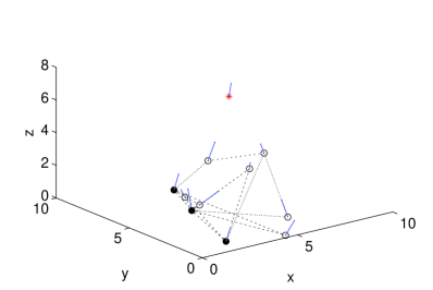
Figure 1: Initial moving state of the group when $N=10$ and $m=3$.

Figure 2: Group’s moving state when $N=10$ and $m=3$ at $t=30$.

The state of position and velocity differences between the agents and the virtual leader are illustrated in Fig. 3 and Fig. 4 respectively. It is shown that the velocities of all the group members converge to the desired velocity. Moreover, the position errors between agents remain fixed after a period of time.

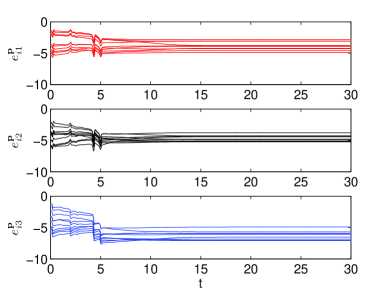
Figure 3: The position differences ${e}_{is}^{\textbf{p}}$ $(1\,\leq\,i\,\leq\,10,\;1\,\leq\,s\,\leq\,3)$ between the agents and the virtual leader when $N=10$ and $m=3$.

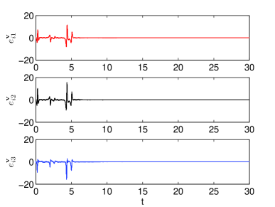
Figure 4: The velocity differences ${e}_{is}^{\textbf{v}}$ $(1\,\leq\,i\,\leq\,10,\;1\,\leq\,s\,\leq\,3)$ between the agents and the virtual leader when $N=10$ and $m=3$.

V-B Flocking in a 200-sized multi-agent group

Large-scale groups with complex topology are common in nature. It has been demonstrated that the topological information of most large-sized systems display scale-free features, among which Barabási and Albert (BA) model [22] of preferential attachment has become the standard mechanism to explain the emergence of scale-free networks. Nodes are added to the network with a preferential bias toward attachment to nodes with already high degree. This naturally gives rise to hubs with a degree distribution following a power-law.

In this subsection, a BA scale-free network consisting of $200$ agents with $q_{0}=5$ and $q=5$ are considered, where $q_{0}$ is the size of the initial network, and $q$ is the number of edges added in each step. Similar to the previous simulation, we take the Lü system as the dynamical acceleration in system (1) and (2). The initial positions and the velocities of the $200$ agents are selected randomly from the cube $[0,50]^{3}$ and $[0,2]^{3}$, and that of the virtual leader are selected as $\textbf{p}_{l}(0)\,=\,(60,60,60)^{\top}$ and $\textbf{v}_{l}(0)\,=\,(1,1,1)^{\top}$. Assume that the other parameters in the simulation are the same as those in the previous subsection.

Denote $\textbf{B}^{BA}_{194}$ as the minor matrix of the adjacent matrix $\textbf{B}^{BA}$ by removing $6$ row-column pairs which corresponds to the $6$ agents with the largest degree in the whole group. Since the maximum eigenvalue of $\textbf{B}^{BA}_{194}$ satisfies

$$\lambda_{max}(\textbf{B}^{BA}_{194})\,=\,-0.9284\,<\,-0.8620\,=\,-\frac{\alpha}{w},$$

the $6$ agents with the largest degrees can be picked out as pseudo-leaders of the group. After using the control mechanism presented in Theorem 1, flocking appears by letting just $3\%$ agents be informed. The moving states of all the group members at $t=0$ and $t=30$ are exhibited in Fig. 5 and Fig. 6.

Clearly, the approaches presented in this paper are of high accuracy with good performance not only for small-sized multi-agent groups but also for larger-scale multi-agent systems.

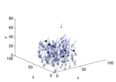
Figure 5: Initial moving state of the group when $N=200$ and $m=6$.

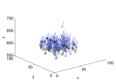
Figure 6: Group’s moving state when $N=200$ and $m=6$ at $t=30$.

VI Conclusions

In this paper, we have presented a criterion for choosing pseudo-leaders in a multi-agent dynamical group. Particularly, the weight configuration of the position and velocity neighbor graph is not necessarily irreducible or time invariant. By combining the ideas of virtual force and pseudo-leader mechanism, mathematical analysis has been deduced to illustrate how to determine the pseudo-leader set in a group. The proposed schemes have been proved rigorously by using Schur complement and Lyapunov stability theory. Finally, two computational examples including small-sized and larger-scale multi-agent groups have been shown to illustrate the effectiveness of the proposed approach.

References

• [1]
• [2] C. W. Reynolds, “Flocks, herds, and schools: a distributed behavioral model,” Computer Graphics, vol. 21, no. 4, pp. 25-34, Jul. 1987.
• [3] T. Vicsek, A. Czirok, E. Ben-Jacob, I. Cohen and O. Shochet, “Novel type of phase transition in a system of self-driven particles,” Phys. Rev. Lett., vol. 75, pp. 1226-1229, Aug. 1995.
• [4] Jackie (Jianhong) Shen, “Cucker-Smale flocking under hierarchical leadership,” SIAM Journal on Applied Mathematics, vol. 68, no. 3, pp. 694-719, 2007.
• [5] H. G. Tanner, A. Jadbabaie and G. J. Pappas, “Stable flocking of mobile agents, part I: fixed topology,” Proc. the 42nd IEEE Conference on Decision and Control, pp. 2010-2015, Dec. 2003.
• [6] H. G. Tanner, A. Jadbabaie and G. J. Pappas, “Stable flocking of mobile agents, part II: dynamic topology,” Proc. the 42nd IEEE Conference on Decision and Control, pp. 2010-2015, Dec. 2003.
• [7] H. G. Tanner, A. Jadbabaie and G. J. Pappas, “Flocking in fixed and switching networks,” IEEE Transactions on Automatic Control, vol. 52, no. 5, pp. 863-868, May. 2007.
• [8] R. Olfati-Saber, “Flocking for multi-agent dynamic systems: algorithms and theory,” IEEE Transactions on Automatic Control, vol. 51, no. 3, pp. 401-420, Mar. 2006.
• [9] H. S. Su, X. F. Wang and Z. L. Lin, “Flocking of multi-agents with a virtual leader, part I: with a minority of informed agents,” Proc. the 46th IEEE Conference on Decision and Control, pp. 2937-2942, Dec. 2007.
• [10] H. S. Su, X. F. Wang and Z. L. Lin, “Flocking of multi-agents with a virtual leader, part II: with a virtual leader of varying velocity,” Proc. the 46th IEEE Conference on Decision and Control, pp. 1429-1434, Dec. 2007.
• [11] H. Shi, L. Wang and T. G. Chu, “Virtual leader approach to coordinated control of multiple mobile agents with asymmetric interactions,” Physica D, vol. 213, pp. 51-65, 2006.
• [12] X. H. Li, J. Z. Xiao and Z. J. Cai, “Stable flocking of swarms using local information,” Proc. IEEE Int. Conf. on Systems, Man and Cybernetics, pp. 3921-3926, Oct. 2005.
• [13] C. Godsil and G. Royle, Algebraic Graph Theory. Springer-Verlag, New York, 2001.
• [14] P. A. Horn and C. R. Johnson, Matrix Analysis. Cambridge University Press, New York, 1985.
• [15] I. S. Gradshteyn and I. M. Ryzhik, Tables of Integrals, Series, and Products. 6th edition, Academic Press, 2000.
• [16] K. K. Hassan, Nonlinear systems. 3rd edition, Prentice Hall, 2002.
• [17] S. Boyd, L. E. Ghaoui, E. Feron and V. Balakrishnan, Linear matrix inequalities in system and control theory. Philadelphia, PA: SIAM, 1994.
• [18] W. W. Yu, J. D. Cao and J. H. Lü, “Global synchronization of linearly hybrid coupled networks with time-varying delay,” SIAM Journal on Applied Dynamical Systems, vol. 7, no. 1, pp. 108-133, 2008.
• [19] T. P. Chen, X. W. Liu and W. L. Lu, “Pinning complex networks by a single controller,” IEEE Trans. Circuits Syst. I, vol. 54, no. 6, pp. 1317-1326, 2007.
• [20] H. Jeffreys and B. S. Jeffreys, Methods of Mathematical Physics. 3rd edition, Cambridge University Press, 1988.
• [21] J. H. Lü, G. Chen, D. Cheng, and S. Celikovsky, “Bridge the gap between the Lorenz system and the Chen system,” International Journal of Bifurcation and Chaos, vol. 12, no. 12, pp. 2917-2926, Dec. 2002.
• [22] A-L. Barab$\acute{a}$si and R. Albert, “Emergence of Scaling in Random Networks,” Science, vol. 286, no. 5439, pp. 509-512, Oct. 1999.
• [23]