Weak-Coupling Limit. I
A Contraction Semigroup for Infinite Subsystems

Abstract

We consider the class of quantum mechanical master equations defined on a generic Banach space, arising by projecting weakly perturbed one-parameter groups of isometries. We show that the possible semigroup approximations are far from unique. However, uniqueness can be reestablished through the introduction of a dynamical time averaging map. The generator of the resulting Contraction Semigroup is always well defined, irrespective of the dimensions of the projected subspace, and of the spectral properties of its free dynamics. We show how our approach includes and generalizes the preexisting literature.

1 Introduction

After the pioneering works in 1974 and 1976 by Davies ([1, 2]), a huge amount of physical information about the irreversibility and the evolution of open quantum mechanical systems has been gained [3]. Alicky [4] showed in 1977 that these efforts were deeply connected to the celebrated ”Fermi’s Golden Rule”, that now had become mathematically consistent. The conceptual importance of these works is clearly not only academic, as the need for a better understanding of irreversible processes has never been more urgent. Today, so many nanotechnologies are pushing devices towards limits where neither quantum phase coherence, nor dissipation/dephasing, can be neglected [5, 6, 7, 8, 9]. Many attempts to improve the theory have been made since then (see for example [10, 11]), but despite the compelling need, no substantial, fundamental progress, directly applicable to nowadays technologies, has been made so far.

To be more specific, the problem is to understand the dynamics of a subsystem of interest, when the global system is fully coherent. In many cases, the dynamics of the global system can be splitted into a part that leaves the subsystem invariant, plus an interaction between the subsystem and the remaining ”unobserved” degrees of freedom. The problem then arises whether or not the subsystem can be given a markovian, possibly dissipative, dynamics as a consequence of its interaction with those degrees of freedom. It has been shown since the ’70s that this problem can be attacked, and partially solved [1, 2], when the amount of unobserved degrees of freedom is huge, and the interaction is made small. This last condition is referred to as the ”weak-coupling limit”.

In [1] the author was able to give a solid physical model of a discrete ”atom” (system A) interacting with a fermionic particle reservoir at thermal equilibrium (environment B). In that case, the subsystem was made of unentangled pairs of atomic states (also referred to as ”density matrices”) and a fermionic thermal equilibrium state, while all the entangled pairs just constituted the remaining, uninteresting, degrees of freedom. The model was of high conceptual importance, as the markovian (and dissipative) dynamics for the subsystem was shown to guarantee the state positivity at all times. This fact gave just enough internal robustness to the model as to be of invaluable practical use, for at any time, the subsystem evolution could be given a strong physical meaning. But the system A had to be finite dimensional, or at least, its unperturbed hamiltonian was forced to have discrete spectrum. This fact constitutes a severe limitation with respect to nowadays needs to explore systems at mesoscopic scale, where energy spectra are often of mixed nature.

Unfortunately, positivity through the weak-coupling limit procedure becomes no more available when the system is infinite dimensional, or the spectrum is continuous. In that case indeed Davies showed that a markovian approximation, for the subsystem exact projected dynamics, could still be achieved [2], but positivity could not be shown even for the old and ”safe” partial tracing over the thermal bath’s degrees of freedom. Being more general, the theory was and is currently applied in many physical urgent contests (see for example [12]), but certainly it did not share the enormous success of the previous one among physicists, precisely because of the serious positivity limitation. For example, all of the steady state analysis became, physically, completely meaningless.

In this work we provide a rigorous solution to this problem in the general contest of Banach spaces, by extending and putting on more firm grounds our initial study in [13]. We suppose the global system is undergoing a fully coherent evolution (according to a perturbed one-parameter group of isometries), and discover a whole class of new markovian approximations for the subsystem, by suitably manipulating the memory kernel of the exact projected evolution, in the limit of small perturbation. This class includes the markovian approximation performed by Davies in [2], and every generator in it is well defined irrespective of the subsystem spectral properties and dimensions. Since we will work in the general contest of Banach spaces, we will not address positivity at this time, but it will be evident that none of generators found so far gives rise to a contraction semigroup, which is a basic requirement for a Quantum Dynamical Semigroup [14] in the more specific contest of $W^{*}$-algebras.

At this point, we will introduce a ”transition time” function, that will scale with the inverse of the perturbation, and will represent physically the transition time among the set of relevant states, due to the perturbation. This time will serve us to perform a ”dynamical average” among all the generators previously found. The result will be a ”dynamical time averaging map”, very similar to the time average proposed in [1], but fundamentally different in that $i)$ it will scale with the coupling constant and $ii)$ it averages among different generators (in [1] the time average acts on one generator only). We shall be able to prove that the resulting transition time dynamically averaged generator $i)$ correctly approximates the exact projected dynamics in the weak-coupling limit, $ii)$ is always well defined, irrespective of the subsystem spectral properties and dimensions, $iii)$ accounts also for first order contributions, $iv)$ boils down to the averaged generator in [1] in case of discrete spectrum, and we shall prove the all important result that $v)$ it gives rise to a contraction semigroup on the projected Banach subspace.

Thus the requirement of a contraction semigroup essentially removes the degeneracy of all the possible semigroup approximations. The generality with which we shall be able to make our statements (no dependence on spectral properties or dimensions of the projected subspace) establishes on firm grounds the possibility of many new important physical (and mathematical) applications.

2 General Theory and Motivation

We report from Davies [2] the general framework we’ll be involved with. We suppose that $P_{0}$ is a linear projection on a Banach space $\mathcal{B}$ (that represents some global system), put $P_{1}=1-P_{0}$ and $\mathcal{B}_{i}=P_{i}\mathcal{B}$, so that

$$\mathcal{B}=\mathcal{B}_{0}\oplus\mathcal{B}_{1},$$ (1)

and we take $\mathcal{B}_{0}$ to represent a subsystem of interest, $\mathcal{B}_{1}$ being the remaining degrees of freedom. We suppose that $Z$ is the (densely defined) generator of a strongly continuous one-parameter group of isometries $U_{t}$ on $\mathcal{B}$ with

$$U_{t}P_{0}=P_{0}U_{t}$$ (2)

for all $t\in\mathbb{R}$, or equivalently

$$[Z,P_{0}]=0$$ (3)

and put $Z_{i}=P_{i}Z$. We suppose that $A$ is a bounded perturbation of $Z$ and put $A_{ij}=P_{i}AP_{j}$. We let $U^{\lambda}_{t}$ be the one parameter group generated by $(Z+\lambda A_{00}+\lambda A_{11})$ so that

$$U^{\lambda}_{t}P_{0}=P_{0}U^{\lambda}_{t}$$ (4)

for all $t\in\mathbb{R}$, and let $V_{t}^{\lambda}$ be the one parameter group generated by $Z+\lambda A$, so that

$$V^{\lambda}_{t}=U^{\lambda}_{t}+\lambda\int_{0}^{t}U^{\lambda}_{t-s}(A_{01}+A_{10})V^{\lambda}_{s}ds.$$ (5)

Then putting

$$X^{\lambda}_{t}=P_{0}U^{\lambda}_{t}$$ (6)

and defining the projected evolution as

$$W^{\lambda}_{t}=P_{0}V^{\lambda}_{t}P_{0}$$ (7)

and one obtains the all important closed and exact integral equation

$$W^{\lambda}_{t}=X^{\lambda}_{t}+\lambda^{2}\int_{0}^{t}ds\int_{0}^{s}du\;X^{\lambda}_{t-s}A_{01}U^{\lambda}_{s-u}A_{10}W^{\lambda}_{u}.$$ (8)

This is nothing but the integrated form of the well known master equation constructed by Nakajima, Prigogine, Resibois, and Zwanzig [15, 16], which follows by repeatedly making use of (5) with

$$W^{\lambda}_{t}=X^{\lambda}_{t}+\lambda\int_{0}^{t}ds\;X^{\lambda}_{t-s}A_{01}V^{\lambda}_{s}P_{0}$$ (9)

and

$$P_{1}V^{\lambda}_{s}P_{0}=\lambda\int_{0}^{s}du\;U^{\lambda}_{s-u}A_{10}W^{\lambda}_{u}.$$ (10)

Now let $X^{\lambda}_{t}$ is a one parameter group of isometries. For example, Davies proves [2] that

Lemma 3

If $\|P_{0}\|=1$ and $\|e^{At}\|=1$ for all $t\in\mathbb{R}$, then $X^{\lambda}_{t}$ is a one parameter group of isometries on $\mathcal{B}_{0}$ for all real $\lambda$.

Then, changing variables to $x=s-u$, $\sigma=\lambda^{2}u$ and introducing the time rescaled (and $A_{00}$-renormalized) interaction picture evolution $W^{\lambda,i}_{\tau}=X_{-\lambda^{-2}\tau}W^{\lambda}_{\lambda^{-2}\tau}$, one is led to [2]:

$$W^{\lambda,i}_{\tau}=1+\int_{0}^{\tau}d\sigma\;X_{-\lambda^{-2}\sigma}^{\lambda}K(\lambda,\tau-\sigma)X_{\lambda^{-2}\sigma}^{\lambda}W^{\lambda,i}_{\sigma}$$ (11)

where

$$K(\lambda,\tau)=\int_{0}^{\lambda^{-2}\tau}X_{-x}A_{01}U^{\lambda}_{x}A_{10}\;dx.$$ (12)

This form separates an ”interacting” and ”slowly varying” part $K(\lambda,\tau)$ from the ”rapidly oscillating” free-evolution $X_{\lambda^{-2}\sigma}$ to second order in the coupling constant $\lambda$. Now in the weak-coupling limit $\lambda\rightarrow 0$, the slowly varying integral kernel $K(\lambda,\tau)$ converges to

$$K_{D}=\int_{0}^{\infty}U_{-x}A_{01}U_{x}A_{10}\;dx\;,$$ (13)

where $K_{D}$ is the celebrated Davies’ superoperator. Substituting $K_{D}\sim K(\lambda,\tau)$ in (11) and moving back to the ”Schrödinger picture” we obtain the markovian approximation for our subsystem dynamics

$${W}^{\lambda}_{t}\approx\overline{W}^{\lambda}_{t}=e^{(Z_{0}+\lambda A_{00}+\lambda^{2}K_{D})t},\quad 0\leq t\leq\lambda^{-2}\tau\quad,\lambda\approx 0$$ (14)

Indeed in [2] an important theorem shows that under reasonable and general conditions the approximation holds in the weak-coupling limit, up to $\lambda^{-2}$-rescaled positive times $\tau$, independently of the subsystem dimensions or spectral properties. Unfortunately, $K_{D}$ does not guarantee positivity of the generated evolution, for example in the case of partial tracing over a bath [1], and thus may fail to furnish a physically acceptable model at times $t>\lambda^{-2}\tau$. This fact precludes the important possibility to study the limit dynamics at all times, together with all the steady state analysis.

However, in [1] the author shows that, in case $\mathcal{B}_{0}$ is finite dimensional (or more generally when $Z_{0}$ has discrete spectrum), one can define a temporal average $K_{D}^{\natural}$ of $K_{D}$ and show that the generated evolution is still asymptotic to the exact one in the weak-limit (at least when $A_{00}=0$). Moreover, the author also shows that if the projection $P_{0}$ is taken to be the partial trace over a bath, the averaged $K_{D}^{\natural}$ generates a Quantum Dynamical Semigroup (QDS) in the sense of [14].

So finally $K_{D}$ does not guarantee a positive evolution at all times, while $K_{D}^{\natural}$ is well defined only in the far too restrictive case of discrete $Z_{0}$-spectrum. This serious problem is physically so important as to motivate our work.

4 Classes of Generators and Dynamical Transition Time

In our first main theorem, we shall look for the most general form of an operator whose evolution is still asymptotic to the exact one in the weak-limit. To this purpose, note that $K_{D}$ has been defined thanks to the change of variable

$$\left(\begin{array}[]{c}s\\ u\end{array}\right)=\left(\begin{array}[]{c c}\lambda^{-2}&1\\ \lambda^{-2}&0\end{array}\right)\left(\begin{array}[]{c}\sigma\\ x\end{array}\right).$$ (15)

Here instead we would like to allow for the most general change of variable that keeps a $\lambda^{-2}$ jacobian, proper of a second order approximation, while fixing the relative variable to be $s-u=x$. So we chose

$$\left(\begin{array}[]{c}s\\ u\end{array}\right)=\left(\begin{array}[]{ccc}\lambda^{-2}&&\alpha+{1\over 2}\\ \lambda^{-2}&&\alpha-{1\over 2}\end{array}\right)\left(\begin{array}[]{c}\sigma-\lambda^{2}q\\ x\end{array}\right),$$ (16)

with inverse

$$\left(\begin{array}[]{c}\sigma\\ x\end{array}\right)=\left(\begin{array}[]{c c c}\left({1\over 2}-\alpha\right)\lambda^{2}&&\left({1\over 2}+\alpha\right)\lambda^{2}\\ 1&&-1\end{array}\right)\left(\begin{array}[]{c}s\\ u\end{array}\right)+\left(\begin{array}[]{c}\lambda^{2}q\\ 0\end{array}\right),$$ (17)

for some real $\alpha$ and $q$. Some straightforward algebra shows that the integration domain $s=0\ldots\lambda^{-2}\tau$, $u=0\ldots s$ in (8), becomes the domain $\mathcal{D}(\lambda,\tau,\alpha,q)$ in the $(\sigma,x)$ plane given by the triangle of vertices

$$\mathcal{D}(\lambda,\tau,\alpha,q)=\triangle\left\{(\lambda^{2}q,0),(\tau+\lambda^{2}q,0),\left(\left({1\over 2}-\alpha\right)\tau+\lambda^{2}q,\lambda^{-2}\tau\right)\right\}$$ (18)

(see figure (1)).

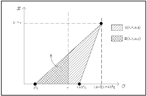
Figure 1: Integration domains $\mathcal{D}(\lambda,\tau,\alpha,q)$ and $\overline{\mathcal{D}}(\lambda,\tau,\alpha,q)$ defined in (18) and (32) respectively (we have put $q>0$ , $\alpha<-1/2$ for clarity). The arrow indicates the asymptotic behavior of the two domains in the weak coupling limit $\lambda\rightarrow 0$ (see discussion in the text following (18)).

Accordingly, equation (8), written for $W^{\lambda,i}_{\tau}=X_{-\lambda^{-2}\tau}W^{\lambda}_{\lambda^{-2}\tau}$, becomes

$$W^{\lambda,i}_{\tau} = 1+\iint\limits_{\mathcal{D}(\lambda,\tau,\alpha,q)}\!\!d\sigma dx\;X^{\lambda}_{-\lambda^{-2}\sigma+q-\left(\alpha+{1\over 2}\right)x}A_{01}U^{\lambda}_{x}A_{10}X^{\lambda}_{\lambda^{-2}\sigma-q+\left(\alpha-{1\over 2}\right)x}$$ (19)

$$\times W^{\lambda,i}_{\sigma-\lambda^{2}(q+(\alpha-1/2)x)}\;.$$

We now consider the following facts, which will be made precise and proven in Theorem 7.1:

• $\mathcal{D}(\lambda,\tau,\alpha,q)\rightarrow[0,\tau]\times[0,\infty)$ as $\lambda\rightarrow 0$, for any real $\alpha$ and $q$. This justifies the approximation

  $$\iint\limits_{\mathcal{D}(\lambda,\tau,\alpha,q)}\!\!\!\!d\sigma\,dx\approx\int_{0}^{\tau}d\sigma\int_{0}^{\infty}dx\;e^{-(x/2)^{2}/T(\lambda)^{2}}\qquad\lambda\approx 0,$$ (20)

  for some real function $T$ of the coupling constant, provided $\lim_{\lambda\rightarrow 0}T(\lambda)=+\infty$. Indeed, exponential factor would not change the asymptotic behavior of the kernel, and would naturally conserve the original character of a bounded integration domain for every nonzero $\lambda$;

• In the weak coupling limit $\lambda\rightarrow 0$ one could approximate

  $$W^{\lambda,i}_{\sigma-\lambda^{2}(q+(\alpha-1/2)x)}\approx W^{\lambda,i}_{\sigma}$$ (21)

  in the integral kernel of (19).

Once all this is proven to be legitimate, equation (19) becomes

$$W^{\lambda,i}_{\tau}\approx 1+\int_{0}^{\tau}d\sigma\;X_{-\lambda^{-2}\sigma}^{\lambda}K_{(\alpha,q,T(\lambda))}X_{\lambda^{-2}\sigma}^{\lambda}W^{\lambda,i}_{\sigma}$$ (22)

or, which is the same,

$$W^{\lambda}_{t}\approx\exp\{(Z_{0}+\lambda A_{00}+\lambda^{2}K_{(\alpha,q,T(\lambda))})t\},$$ (23)

where we give the following

Definition 5

Let $\alpha,q\in\mathbb{R}$ be two given real numbers, and let $T\in\mathcal{C}([-1,1],\overline{\mathbb{R}})$ be a real valued positive continuous function on the interval $[-1,1]$, where $\overline{\mathbb{R}}=\mathbb{R}\cup\{\infty\}$. For $\lambda\in I$ define the linear operator $K_{(\alpha,q,T(\lambda))}$ on $\mathcal{B}_{0}$ as

$$K_{(\alpha,q,T(\lambda))}=\int_{0}^{\infty}dx\;e^{-\left({x\over 2}\right)^{2}/T(\lambda)^{2}}\;U_{-\left(\alpha+{1\over 2}\right)x+q}A_{01}U_{x}A_{10}U_{\left(\alpha-{1\over 2}\right)x-q}\;.$$ (24)

Denote also with

$$\overline{W}^{\lambda}_{t}=\exp\{(Z_{0}+\lambda A_{00}+\lambda^{2}K_{(\alpha,q,T(\lambda))})t\}$$ (25)

the associated semigroup on $\mathcal{B}_{0}$.

Then, under fairly general hypotheses, we shall prove that $\overline{W}^{\lambda}_{t}$ is compatible with the exact $W^{\lambda}_{t}$ in the weak coupling limit $\lambda\rightarrow 0$, up to $\lambda^{-2}$-rescaled positive times $\tau$:

$$\lim_{\lambda\rightarrow 0}\left\{\sup_{0\leq t\leq\lambda^{-2}\overline{\tau}}\|W^{\lambda}_{t}-\overline{W}^{\lambda}_{t}\|\right\}=0.$$ (26)

We stress that, as in [2], we do not assume that $\mathcal{B}_{0}$ is finite-dimensional.

The following lemma is not new, and for example it is contained in Theorem 1.2 of [2], but we report it here as we shall make use of it repeatedly all throughout.

Lemma 6

Let $b\in\mathcal{B}_{0}$ be given, together with some real $\overline{\tau}>0$. Suppose $W^{\lambda}_{t}$ and $\overline{W}^{\lambda}_{t}$ are operators on $\mathcal{B}_{0}$ such that $f_{\lambda}(\tau)=X^{\lambda}_{-\lambda^{-2}\tau}W^{\lambda}_{\lambda^{-2}\tau}b$ satisfies

$$f_{\lambda}=\sum_{n\geq 0}\mathcal{H}_{\lambda}^{n}b$$ (27)

for a Volterra operator $\mathcal{H}_{\lambda}$ on the Banach space $\mathcal{V}=\mathcal{C}^{0}([0,\overline{\tau}],\mathcal{B}_{0})$ of continuous $\mathcal{B}_{0}$-valued functions on the interval $[0,\overline{\tau}]$ (assume the same holds also for $\overline{W}^{\lambda}_{t}$, with associated $\overline{f}_{\lambda}$ and $\overline{\mathcal{H}}_{\lambda}$). Suppose there exists a real positive $c$ such that $\|\mathcal{H}_{\lambda}\|_{{}_{\mathcal{V}}}\leq c\overline{\tau}$ and $\|\overline{\mathcal{H}}_{\lambda}\|_{{}_{\mathcal{V}}}\leq c\overline{\tau}$ uniformly on $|\lambda|\leq 1$. Put

$$\begin{array}[]{ll}i)&\lim_{\lambda\rightarrow 0}\|\mathcal{H}_{\lambda}-\overline{\mathcal{H}}_{\lambda}\|_{{}_{\mathcal{V}}}=0\;;\\ ii)&\lim_{\lambda\rightarrow 0}\|f_{\lambda}-\overline{f}_{\lambda}\|_{\infty}=0\;;\\ iii)&\lim_{\lambda\rightarrow 0}\;\sup_{0\leq t\leq\lambda^{-2}\overline{\tau}}\;\|W^{\lambda}_{t}b-\overline{W}^{\lambda}_{t}b\|_{{}_{\mathcal{B}_{0}}}=0\;.\end{array}$$ (28)

Then $i)\Rightarrow ii)\Rightarrow iii)$.

Proof. Of course $ii)\Rightarrow iii)$ as $X^{\lambda}_{t}$ is group of isometries and one has

$$\sup_{0\leq t\leq\lambda^{-2}\overline{\tau}}\|W^{\lambda}_{t}b-\overline{W}^{\lambda}_{t}b\|_{{}_{\mathcal{B}_{0}}}=\sup_{0\leq\tau\leq\overline{\tau}}\;\|f_{\lambda}(\tau)-\overline{f}_{\lambda}(\tau)\|_{{}_{\mathcal{B}_{0}}}=\|f_{\lambda}-\overline{f}_{\lambda}\|_{\infty}\;.$$ (29)

Then, subtracting the von Newmann expansions for $f_{\lambda}$ and $\overline{f}_{\lambda}$ one obtains

$$\|f_{\lambda}-\overline{f}_{\lambda}\|_{\infty}\leq\sum_{n=1}^{\infty}\|\mathcal{H}_{\lambda}^{n}b-\overline{\mathcal{H}}_{\lambda}^{n}b\|_{\infty}$$ (30)

$$= \sum_{n=1}^{\infty}\|\mathcal{H}_{\lambda}^{n}b-\mathcal{H}_{\lambda}^{n-1}\overline{\mathcal{H}}_{\lambda}b+\mathcal{H}_{\lambda}^{n-1}\overline{\mathcal{H}}_{\lambda}b-\cdots+\mathcal{H}_{\lambda}\overline{\mathcal{H}}_{\lambda}^{n-1}b-\overline{\mathcal{H}}_{\lambda}^{n}b\|_{\infty}$$

$$= \sum_{n=1}^{\infty}\|\mathcal{H}_{\lambda}^{n-1}(\mathcal{H}_{\lambda}-\overline{\mathcal{H}}_{\lambda})b+\mathcal{H}_{\lambda}^{n-2}(\mathcal{H}_{\lambda}-\overline{\mathcal{H}}_{\lambda})\overline{\mathcal{H}}_{\lambda}b+\cdots+(\mathcal{H}_{\lambda}-\overline{\mathcal{H}}_{\lambda})\overline{\mathcal{H}}_{\lambda}^{n-1}b\|_{\infty}$$

$$\leq \|\mathcal{H}_{\lambda}-\overline{\mathcal{H}}_{\lambda}\|_{{}_{\mathcal{V}}}\|b\|_{{}_{\mathcal{B}_{0}}}\sum_{n=1}^{\infty}{(\overline{\tau}\>c)^{n-1}\over(n-1)!}$$

and the last series is (obviously) convergent and independent of $\lambda$. Note that we have used (and will use throughout) the important property that if $\mathcal{H}$ is Volterra and $\|\mathcal{H}\|\leq C$, then $\|\mathcal{H}\|^{n}\leq C^{n}/n!$.

This shows that $i)\Rightarrow ii)$ and thus finishes the proof. $\quad\Box$

We still need a technical but important result, that will allow us to perform approximation (21): its interpretation will become clear in the context of Theorem 7.1, but it deserves to be reported in the more autonomous environment of a Lemma, as it will find application also in our second main result, Theorem 9.1.

Lemma 7

Let $\mathcal{B}_{0}$ be a Banach space, $\overline{\tau}>0$, and let $\mathcal{V}=\mathcal{C}^{0}([0,\overline{\tau}],\mathcal{B}_{0})$ be the Banach space of continuous functions from $[0,\overline{\tau}]$ into $\mathcal{B}_{0}$. For some real $q$ and $\alpha$, let $\mathcal{D}(\lambda,\tau,\alpha,q)$ be the triangle in the $(\sigma,x)$-plane of vertices

$$\mathcal{D}(\lambda,\tau,\alpha,q)=\triangle\left\{(\lambda^{2}q,0),(\tau+\lambda^{2}q,0),\left(\left({1\over 2}-\alpha\right)\tau+\lambda^{2}q,\lambda^{-2}\tau\right)\right\}$$ (31)

and define the truncated domain (see figure (1))

$$\overline{\mathcal{D}}(\lambda,\tau,\alpha,q)=\mathcal{D}(\lambda,\tau,\alpha,q)\cap[0,\tau]\times[0,\infty).$$ (32)

Let $T\in\mathcal{C}([-1,1],\overline{\mathbb{R}})$ be a real valued positive continuous function on the interval $[-1,1]$, and assume that $T(\lambda)\sim|\lambda|^{\xi}$ for $\lambda\rightarrow 0$ with $\xi<2$. Let $\mathcal{H}_{(\lambda\alpha q)}$ be a Volterra integral operator on $\mathcal{V}$ and assume it can be put in the form

$$(\mathcal{H}_{(\lambda\alpha q)}g)(\tau)=\int\!\!\!\!\!\!\!\!\!\!\!\!\int\limits_{\overline{\mathcal{D}}(\lambda,\tau,\alpha,q)}\!\!\!\!\!\!d\sigma dx\;e^{-{(x/2)^{2}\over T(\lambda)^{2}}}\;K_{\alpha q}(\lambda,\sigma,x)\>g\left(\sigma-\lambda^{2}\left(q+\left(\alpha-{1/2}\right)x\right)\right),$$ (33)

for a suitable kernel $K_{\alpha q}(\lambda,\sigma,x)$, and define the Volterra integral operator $\overline{\mathcal{H}}_{(\lambda\alpha q)}$ by

$$(\overline{\mathcal{H}}_{(\lambda\alpha q)}g)(\tau)=\int\!\!\!\!\!\!\!\!\!\!\!\!\int\limits_{\overline{\mathcal{D}}(\lambda,\tau,\alpha,q)}\!\!\!\!\!\!d\sigma dx\;e^{-{(x/2)^{2}\over T(\lambda)^{2}}}\;K_{\alpha q}(\lambda,\sigma,x)\>g(\sigma).$$ (34)

Suppose that $\|K_{\alpha q}(\lambda,\sigma,x)\|=k(x)$ independently on $\sigma,\lambda,\alpha,q$, and that

$$\int_{0}^{\infty}dx\;k(x)=c$$ (35)

for some finite $0<c<\infty$, and assume $\|\mathcal{H}_{(\lambda\alpha q)}\|<\overline{\tau}c$.

Let $b\in\mathcal{B}_{0}$ and define the von Neumann series $f_{(\lambda\alpha q)}$ and $\overline{f}_{(\lambda\alpha q)}$ through equation (27) in Lemma (6).

Then

$$\|\overline{\mathcal{H}}_{(\lambda\alpha q)}\|\leq\overline{\tau}c$$ (36)

and

$$\lim_{\lambda\rightarrow 0}\|f_{(\lambda\alpha q)}-\overline{f}_{(\lambda\alpha q)}\|_{\infty}=0\;.$$ (37)

Proof. Estimation (36) is a trivial consequence of the definition of $\overline{\mathcal{H}}_{(\lambda\alpha q)}$, as

$$\|\overline{\mathcal{H}}_{(\lambda\alpha q)}g(\tau)\|\leq\tau\int_{0}^{\infty}k(x)\|g\|_{\infty}.$$ (38)

To show the validity of (37) we start proceeding as in Lemma 6 to obtain

$$\|f_{(\lambda\alpha q)}-\overline{f}_{(\lambda\alpha q)}\|_{\infty}\\ \leq\sum_{n=1}^{\infty}\;\sum_{l=1}^{n-1}\;{(\overline{\tau}\>c)^{n-l-1}\over(n-l)!}\;\|(\mathcal{H}_{(\lambda\alpha q)}-\overline{\mathcal{H}}_{(\lambda\alpha q)})\>\overline{\mathcal{H}}_{(\lambda\alpha q)}^{l}\>b\|_{\infty}\;.$$

Note that the case $l=0$ has been dropped, since $\mathcal{H}_{(\lambda\alpha q)}b=\overline{\mathcal{H}}_{(\lambda\alpha q)}b$ trivially, as $b$ is constant, as one can see from (33). Now if we could show that for every $\epsilon>0$ there exists some $\overline{\lambda}>0$ such that $|\lambda|<\overline{\lambda}$ implies that for every $l\geq 1$

$$\|(\mathcal{H}_{(\lambda\alpha q)}-\overline{\mathcal{H}}_{(\lambda\alpha q)})\>\overline{\mathcal{H}}_{(\lambda\alpha q)}^{l}\>b\|_{\infty}\leq{(\overline{\tau}\>c)^{l-1}\over(l-1)!}\>\overline{\tau}\;\|b\|_{\mathcal{B}_{0}}\>\epsilon\;,$$ (39)

we would be done, as, following estimation (4), we would have

$$\|f_{\lambda}-\overline{f}_{\lambda}\|_{\infty}\leq\sum_{n=1}^{\infty}\;\sum_{l=1}^{n-1}\;{(\overline{\tau}\>c)^{n-2}\over(n-l)!(l-1)!}\>\overline{\tau}\;\|b\|_{\mathcal{B}_{0}}\>\epsilon\;,$$ (40)

and the series would obviously converge (because $c>0$ by hypothesis).

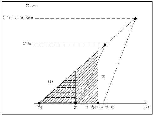
Figure 2: Integration domains $\overline{\mathcal{D}}(\lambda,\sigma,\alpha,q)$ (rectangular triangle $(1)$), $\overline{\mathcal{D}}(\lambda,\sigma-\lambda^{2}\left(q+\left(\alpha-{1\over 2}\right)x\right),\alpha,q)$ (rectangular triangle $(2)$) and $S(\lambda,\sigma,x)$ (region $(1)\cup(2)$). We have put $\alpha<-1/2$, $q>0$ for clarity. The two truncated triangles $\overline{\mathcal{D}}$ are similar, as are also the untruncated, underlying $\mathcal{D}$. Note the scaling behavior with $\lambda^{2}$.

To show that property (39) holds, we take $l>0$ and evaluate

$$\left[(\mathcal{H}_{(\lambda\alpha q)}-\overline{\mathcal{H}}_{(\lambda\alpha q)})\>\overline{\mathcal{H}}_{(\lambda\alpha q)}^{l}\>b\right](\tau)$$ (41)

$$= \iint\limits_{\overline{\mathcal{D}}(\lambda,\tau,\alpha,q)}\!\!\!\!\!\!d\sigma dx\;e^{-{(x/2)^{2}\over T(\lambda)^{2}}}\;K_{\alpha q}(\lambda,\sigma,x)$$

$$\times\left\{(\overline{\mathcal{H}}_{(\lambda\alpha q)}^{l}\>b)\left(\sigma-\lambda^{2}(q+(\alpha-1/2)x)\right)-(\overline{\mathcal{H}}_{(\lambda\alpha q)}^{l}\>b)(\sigma)\right\}$$

$$= \iint\limits_{\overline{\mathcal{D}}(\lambda,\tau,\alpha,q)}d\sigma dx\;e^{-{(x/2)^{2}\over T(\lambda)^{2}}}\;K_{\alpha q}(\lambda,\sigma,x)$$

$$\times\iint\limits_{S(\lambda,\alpha,q,\sigma,x)}d\sigma_{1}dx_{1}\,\Delta^{\lambda}(\sigma_{1},x_{1})\,e^{-{(x/2)^{2}\over T(\lambda)^{2}}}\;K_{\alpha q}(\lambda,\sigma_{1},x_{1})\,(\overline{\mathcal{H}}_{(\lambda\alpha q)}^{l-1}b)(\sigma_{1})$$

where we have put $\Delta^{\lambda}=\chi^{\lambda}_{1}-\chi^{\lambda}_{2}$, $\chi^{\lambda}_{1}$ being the characteristic function of $\overline{\mathcal{D}}(\lambda,\sigma-\lambda^{2}\left(q+\left(\alpha-{1\over 2}\right)x\right),\alpha,q)$, $\chi^{\lambda}_{2}$ the characteristic function of $\overline{\mathcal{D}}(\lambda,\sigma,\alpha,q)$, and we have defined (see Figure 2)

$$S(\lambda,\alpha,q,\sigma,x)=\overline{\mathcal{D}}\left(\lambda,\sigma-\lambda^{2}\left(q+\left(\alpha-{1\over 2}\right)x\right),\alpha,q\right)\cup\overline{\mathcal{D}}(\lambda,\sigma,\alpha,q)\;.$$ (42)

Passing to the norms, we estimate the left hand side of (39) as

$$\|(\mathcal{H}_{\lambda}-\overline{\mathcal{H}}_{(\lambda\alpha q)})\>\overline{\mathcal{H}}_{(\lambda\alpha q)}^{l}\>b\|$$

$$\leq \sup_{0\leq\tau\leq\overline{\tau}}\iint\limits_{\overline{\mathcal{D}}(\lambda,\tau,\alpha,q)}\!\!\!\!\!\!d\sigma dx\,e^{-{(x/2)^{2}\over T(\lambda)^{2}}}\,k(x)\iint\limits_{S(\lambda,\alpha,q,\sigma,x)}\!\!\!d\sigma_{1}dx_{1}\,|\Delta^{\lambda}(\sigma_{1},x_{1})|\,k(x_{1})\,\left\|\overline{\mathcal{H}}_{(\lambda\alpha q)}^{l-1}b\right\|_{\infty}$$

$$\leq {(\overline{\tau}\>c)^{l-1}\over(l-1)!}\>\|b\|_{\mathcal{B}_{0}}\sup_{0\leq\tau\leq\overline{\tau}}\iint\limits_{\overline{\mathcal{D}}(\lambda,\tau,\alpha,q)}\!\!\!\!\!\!d\sigma dx\,e^{-{(x/2)^{2}\over T(\lambda)^{2}}}\,k(x)\;\Xi(\lambda,\sigma,x)\,$$

$$\leq {(\overline{\tau}\>c)^{l-1}\over(l-1)!}\>\|b\|_{\mathcal{B}_{0}}\overline{\tau}\sup_{0\leq\sigma\leq\overline{\tau}}\int_{0}^{\infty}dx\;e^{-{(x/2)^{2}\over T(\lambda)^{2}}}k(x)\;\Xi_{\alpha q}(\lambda,\sigma,x)\,$$

where we named

$$\Xi_{\alpha q}(\lambda,\sigma,x)=\iint\limits_{S(\lambda,\alpha,q,\sigma,x)}\!\!\!d\sigma_{1}dx_{1}\,|\Delta^{\lambda}(\sigma_{1},x_{1})|\,k(x_{1})$$ (44)

At this point let us consider the sector defined by $q>0$ and $\alpha<-1/2$. In this case, it is but a straightforward algebra to show that the two triangles ${\mathcal{D}}\left(\lambda,\sigma-\lambda^{2}\left(q+\left(\alpha-{1\over 2}\right)x\right),\alpha,q\right)$ and ${\mathcal{D}}(\lambda,\sigma,\alpha,q)$ (the same applies to $\overline{\mathcal{D}}$) are similar, and that their left edges lie on the same line of equation

$$\overline{x}_{l}(\lambda,\sigma_{1})={\lambda^{-2}\over{1\over 2}-\alpha}(\sigma_{1}-\lambda^{2}q)$$ (45)

in the $(\sigma_{1},x_{1})$-plane (see figure (2)). In particular,

$$\overline{\mathcal{D}}\left(\lambda,\sigma-\lambda^{2}\left(q+\left(\alpha-{1\over 2}\right)x\right),\alpha,q\right)\;\begin{array}[]{c}\supseteq\\ \subset\end{array}\;\overline{\mathcal{D}}(\lambda,\sigma,\alpha,q),\quad x\gtreqless{q\over{1\over 2}-\alpha}\\$$

For this reason we easily compute

$$\Xi_{\alpha q}(\lambda,\sigma,x)={\rm{sign}}\left(\left({1\over 2}-\alpha\right)x-q\right)\int_{\sigma}^{\sigma-\lambda^{2}\left(q+\left(\alpha-{1\over 2}\right)x\right)}\!\!\!\!\!\!\!\!\!\!\!\!d\sigma_{1}\int_{0}^{\overline{x}_{l}(\lambda,\sigma_{1})}\!\!\!\!\!\!dx_{1}\;k(x_{1})$$

$$\leq\lambda^{2}\left|q+\left(\alpha-{1\over 2}\right)x\right|\int_{0}^{\infty}dx_{1}\;k(x_{1})$$

$$\leq c\lambda^{2}\left(|q|+\left|\alpha-{1\over 2}\right|x\right)$$ (46)

According to the last line in estimation (4), we study

$$\sup_{0\leq\sigma\leq\overline{\tau}}\int_{0}^{\infty}dx\;e^{-{(x/2)^{2}\over T(\lambda)^{2}}}k(x)\;\Xi_{\alpha q}(\lambda,\sigma,x)$$

$$\leq c^{2}\lambda^{2}q+c\left|\alpha-{1\over 2}\right|\int_{0}^{\infty}dx\;k(x)e^{-{(x/2)^{2}\over T(\lambda)^{2}}}\lambda^{2}x$$ (47)

The first term goes to zero with velocity $\sim\lambda^{2}q$, whereas the dominated convergence theorem applies to the second term, showing convergence to zero uniformly on $q$, with velocity $\sim\lambda^{2-\xi}$ (note that we have supposed $\xi<2$ strictly). This, when put in (4), shows the validity of (39).

A very similar analysis can be done for the remaining sectors $q\lesseqgtr 0$, $|\alpha|<1/2$ and $\alpha>1/2$. In each case, the net result is that the estimation (4) is always of the form

$$\sup_{0\leq\sigma\leq\overline{\tau}}\int_{0}^{\infty}dx\;e^{-{(x/2)^{2}\over T(\lambda)^{2}}}k(x)\;\Xi_{\alpha q}(\lambda,\sigma,x)\;\leq\;C_{1}\lambda^{2}|q|+C_{2}\lambda^{2-\xi}$$ (48)

for suitable real positive constants $C_{1}$ and $C_{2}$. Again, this shows the validity of (39), and thus concludes the proof. $\quad\Box$

We are now in position to state our first main result:

Theorem 7.1

Suppose that $X^{\lambda}_{t}$ is a one-parameter group of isometries.

Let $T\in\mathcal{C}([-1,1],\overline{\mathbb{R}})$ be a real valued positive continuous function on the interval $[-1,1]$, and assume

$$T(\lambda)\sim|\lambda|^{-\xi}\widetilde{T},\quad\lambda\rightarrow 0$$ (49)

for some real positive $\widetilde{T}>0$ and $0<\xi<2$ (strictly).

Suppose that there exists some $0<c<\infty$ such that for every $\overline{\tau}>0$

$$\int_{0}^{\lambda^{-2}\overline{\tau}}\|A_{01}U^{\lambda}_{x}A_{10}\|\,dx\leq c$$ (50)

is bounded uniformly on $|\lambda|\leq 1$.

Suppose also that for every $0<\overline{\tau}<\infty$

$$\lim_{\lambda\rightarrow 0}\int_{0}^{\lambda^{-2}\overline{\tau}}\|A_{01}(U^{\lambda}_{x}-U_{x})A_{10}\|\,dx=0\;.$$ (51)

Then for every $\overline{\tau}>0$

$$\lim_{\lambda\rightarrow 0}\left\{\sup_{0\leq t\leq\lambda^{-2}\overline{\tau}}\|W^{\lambda}_{t}-\overline{W}^{\lambda}_{t}\|\right\}=0.$$ (52)

Proof. Let $\mathcal{V}$ be the Banach space of norm continuous $\mathcal{B}_{0}$-valued functions on $[0,\overline{\tau}]$, and let $b\in\mathcal{B}_{0}$. Define the ”interaction picture” time rescaled solution of (8)

$$f_{\lambda}(\tau)=X^{\lambda}_{-\lambda^{-2}\tau}W^{\lambda}_{\lambda^{-2}\tau}b.$$ (53)

Then $f_{\lambda}$ is a solution to the integral equation

$$f_{\lambda}=b+\mathcal{H}_{\lambda}f_{\lambda},$$ (54)

where the integral operator $\mathcal{H}_{\lambda}$ is defined (recall that $X^{\lambda}_{t}$ is a group of isometries) by

$$(\mathcal{H}_{\lambda}g)(\tau)=\lambda^{2}\int_{0}^{\lambda^{-2}\tau}\!\!\!\!ds\int_{0}^{s}du\;X^{\lambda}_{s}A_{01}U^{\lambda}_{s-u}A_{10}X^{\lambda}_{u}\;g(\lambda^{2}u)\;.$$ (55)

In [2] Davies shows that $\mathcal{H}_{\lambda}$ is a Volterra operator. Indeed, by changing coordinates according to (15), Eq. (55) can be given an explicit Volterra form, namely as

$$(\mathcal{H}_{\lambda}g)(\tau)=\int_{0}^{\tau}d\sigma X^{\lambda}_{-\lambda^{-2}\sigma}K(\lambda,\tau-\sigma)X^{\lambda}_{\lambda^{-2}\sigma}\;g(\sigma)\;,$$ (56)

where we defined the ”slowly varying” kernel

$$K(\lambda,\tau)=\int_{0}^{\lambda^{-2}\tau}dx\;X^{\lambda}_{-x}A_{01}U^{\lambda}_{x}A_{10}.$$ (57)

Because of this reason, and since $K(\lambda,\tau)$ is manifestly bounded by $c$, uniformly on $\lambda$ (thanks our boundedness hypothesis), it follows that

$$\|\mathcal{H}_{\lambda}^{n}\|\leq c^{n}\overline{\tau}^{n}/n!,$$ (58)

and also that the associated von Newmann series expansion

$$f_{\lambda}=b+\mathcal{H}_{\lambda}b+\mathcal{H}_{\lambda}^{2}b+\cdots$$ (59)

converges.

We can proceed in similar fashion also for the semigroup (25): iteration gives indeed

$$\overline{W}^{\lambda}_{\lambda^{-2}\tau}=X^{\lambda}_{-\lambda^{-2}\tau}+\int_{0}^{\tau}d\sigma\;X^{\lambda}_{-\lambda^{-2}(\tau-\sigma)}K_{(\alpha,q,T(\lambda))}W^{\lambda}_{\lambda^{-2}\sigma}\;.$$ (60)

Accordingly, we define

$$\overline{f}_{\lambda}(\tau)=X^{\lambda}_{-\lambda^{-2}\tau}\overline{W}^{\lambda}_{\lambda^{-2}\tau}b$$ (61)

so that it follows that $\overline{f}_{\lambda}$ is a solution to the integral equation

$$\overline{f}_{\lambda}=b+\overline{\mathcal{H}}_{(\lambda\alpha q)}\overline{f}_{\lambda},$$ (62)

where we have defined

$$(\overline{\mathcal{H}}_{(\lambda\alpha q)}g)(\tau)=\int_{0}^{\tau}d\sigma\;X^{\lambda}_{-\lambda^{-2}\sigma}K_{(\alpha,q,T(\lambda))}X^{\lambda}_{\lambda^{-2}\sigma}g(\sigma).$$ (63)

Now again, $\overline{\mathcal{H}}_{(\lambda\alpha q)}$ is a Volterra operator, and since $\|K_{\alpha,q}\|\leq c$, equations (58) and (59) follow analogously for $\overline{\mathcal{H}}_{(\lambda\alpha q)}$.

Clearly (see Lemma 6), we must show that for any chosen $b\in\mathcal{B}_{0}$,

$$\sup_{0\leq t\leq\lambda^{-2}\overline{\tau}}\|W^{\lambda}_{t}b-\overline{W}^{\lambda}_{t}b\|=\|f_{\lambda}-\overline{f}_{\lambda}\|_{\infty}\rightarrow 0,\quad\lambda\rightarrow 0.$$ (64)

We shall do that by defining suitable Volterra operators, denoted with $\mathcal{H}^{(j)}_{(\lambda\alpha q)}$, $j=0\ldots N$, such that $\mathcal{H}^{(0)}_{(\lambda\alpha q)}=\mathcal{H}_{\lambda}$, $\mathcal{H}^{(N)}_{(\lambda\alpha q)}=\overline{\mathcal{H}}_{(\lambda\alpha q)}$, and either we can show, according to Lemma 6, that

$$\|\mathcal{H}^{(j)}_{(\lambda\alpha q)}-\mathcal{H}^{(j-1)}_{(\lambda\alpha q)}\|_{{}_{\mathcal{V}}}\rightarrow 0\;,\quad\lambda\rightarrow 0$$ (65)

or more directly that

$$\|f^{(j)}_{(\lambda\alpha q)}-f^{(j-1)}_{(\lambda\alpha q)}\|_{\infty}\rightarrow 0\;,\quad\lambda\rightarrow 0$$ (66)

where

$$f^{(j)}_{(\lambda\alpha q)}=\sum_{n=0}^{\infty}\left(\mathcal{H}^{(j)}_{(\lambda\alpha q)}\right)^{n}b$$ (67)

is the associated von Neumann series. Then, our conclusion (see Lemma 6) would follow from

$$\|f_{\lambda}-\overline{f}_{\lambda}\|\leq\sum_{j=1}^{N}\|f^{(j)}_{(\lambda\alpha q)}-f^{(j-1)}_{(\lambda\alpha q)}\|\rightarrow 0\quad\lambda\rightarrow 0.$$ (68)

To follow our purpose, instead of (15), we perform the coordinate transformations (16) As we noted before, the integration domain $s=0\ldots\lambda^{-2}\tau$, $u=0\ldots s$, becomes the domain $\mathcal{D}(\lambda,\tau,\alpha,q)$ in the $(\sigma,x)$-plane defined in (18), and depicted in figure (1). Accordingly, the integral kernel in (55) is now written as

$$(\mathcal{H}_{\lambda}g)(\tau) = \iint\limits_{\mathcal{D}(\lambda,\tau,\alpha,q)}\!\!d\sigma dx\;X^{\lambda}_{-\lambda^{-2}\sigma+q-\left(\alpha+{1\over 2}\right)x}A_{01}U^{\lambda}_{x}A_{10}X^{\lambda}_{\lambda^{-2}\sigma-q+\left(\alpha-{1\over 2}\right)x}$$ (69)

$$\times g(\sigma-\lambda^{2}(q+(\alpha-{1/2})x))\;.$$

We shall work throughout with the choice $\alpha<-1/2$ and $q>0$, without loss of generality (the structure of the proof is basically the same for all the remaining sectors, which we leave to the reader, and actually the case $|\alpha|<1/2$ presents less difficulties).

The first thing we shall be concerned with, is to find a way to substitute the free ”polarization evolution” $P_{1}U_{x}$ in place of the interacting $P_{1}U^{\lambda}_{x}$ in the middle of the kernel in (69). This step is accomplished by defining a related integral operator $\mathcal{H}^{(1)}_{\lambda}$ by

$$(\mathcal{H}^{(1)}_{(\lambda\alpha q)}g)(\tau) = \iint\limits_{\mathcal{D}_{(1)}(\lambda,\tau,\alpha,q)}\!\!\!d\sigma dx\;X^{\lambda}_{-\lambda^{-2}\sigma+q-\left({\alpha+1\over 2}\right)x}A_{01}U_{x}A_{10}X^{\lambda}_{\lambda^{-2}\sigma-q+\left(\alpha-{1\over 2}\right)x}$$ (70)

$$\times g(\sigma-\lambda^{2}(q+(\alpha-{1/2})x))\;.$$

Here we have denoted $\mathcal{D}_{(1)}=\mathcal{D}$ for sake of notation. Note that $\mathcal{H}^{(1)}_{(\lambda\alpha q)}$ does not depend on $\alpha$, nor on $q$, although both the latter parameters appear in its definition. To compare the two integral operators, take a bounded $g\in\mathcal{V}$ and estimate

$$\left\|\>\left(\mathcal{H}_{\lambda}-\mathcal{H}^{(1)}_{(\lambda\alpha q)}\right)g\>\right\|\;\leq\;\iint\limits_{\mathcal{D}(\lambda,\tau,\alpha,q)}\!\!\!d\sigma dx\;\|A_{01}(U^{\lambda}_{x}-U_{x})A_{10}\|\;\|g\|_{\infty}$$

$$\leq\max\{1,|1/2-\alpha|\}\;\overline{\tau}\|g\|_{\infty}\int_{0}^{\lambda^{-2}\overline{\tau}}\!\!\!\!\!dx\;\|A_{01}(U^{\lambda}_{x}-U_{x})A_{10}\|$$ (71)

(note for later purposes that the estimation does not depend on $q$). Our convergence hypothesis (51) on $U^{\lambda}_{x}$ allows then to conclude that this goes to zero when $\lambda\rightarrow 0$ uniformly on every $\|g\|=1$, so that we obtain

$$\lim_{\lambda\rightarrow 0}\left\|\>\mathcal{H}_{\lambda}-\mathcal{H}^{(1)}_{(\lambda\alpha q)}\>\right\|=0\;.$$ (72)

We proceed along similar lines to smooth the kernel with $T(\lambda)$: define

$$(\mathcal{H}^{(2)}_{(\lambda\alpha q)}g)(\tau) = \!\!\!\iint\limits_{\mathcal{D}_{(2)}(\lambda,\tau,\alpha,q)}\!\!\!\!\!d\sigma dx\;e^{-{(x/2)^{2}\over T(\lambda)^{2}}}\;X^{\lambda}_{-\lambda^{-2}\sigma+q-\left(\alpha+{1\over 2}\right)x}A_{01}U_{x}A_{10}X^{\lambda}_{\lambda^{-2}\sigma-q+\left(\alpha-{1\over 2}\right)x}$$ (73)

$$\times g(\sigma-\lambda^{2}(q+(\alpha-{1/2})x))\;.$$

Here we have denoted $\mathcal{D}_{(2)}=\mathcal{D}_{(1)}$. To compare with $\mathcal{H}^{(1)}_{(\lambda\alpha q)}$, take a bounded $g\in\mathcal{V}$ and estimate

$$\left\|\>\left(\mathcal{H}^{(1)}_{(\lambda\alpha q)}-\mathcal{H}^{(2)}_{(\lambda\alpha q)}\right)g\>\right\|\leq\iint\limits_{\mathcal{D}(\lambda,\tau,\alpha,q)}\!\!\!d\sigma dx\;|1-e^{-({x\over 2})^{2}/T(\lambda)^{2}}|\;\|A_{01}U_{x}A_{10}\|\;\|g\|_{\infty}$$

$$\leq\max\left\{1,\left|{1\over 2}-\alpha\right|\right\}\;\overline{\tau}\|g\|_{\infty}\int_{0}^{\infty}dx\;|1-e^{-{(x/2)^{2}\over T(\lambda)^{2}}}|\;\|A_{01}U_{x}A_{10}\|$$ (74)

Hypothesis (50) furnishes an integrable upper bound to the last integrand, and so the integral goes to zero in the limit $\lambda\rightarrow 0$ because of the dominated convergence theorem: in fact, one has pointwise convergence

$$\left|1-e^{-{(x/2)^{2}\over T(\lambda)^{2}}}\right|\rightarrow 0,\quad\lambda\rightarrow 0\;$$ (75)

due to our hypothesis $0<\xi$. Uniform convergence on all $\|g\|=1$ in the last line of our estimation then shows that

$$\lim_{\lambda\rightarrow 0}\left\|\>\mathcal{H}^{(1)}_{(\lambda\alpha q)}-\mathcal{H}^{(2)}_{(\lambda\alpha q)}\>\right\|=0\;.$$ (76)

We note that $\mathcal{H}^{(2)}_{(\lambda\alpha q)}$, as $\mathcal{H}^{(1)}_{(\lambda\alpha q)}$ and $\mathcal{H}_{\lambda}$, is also a Volterra operator, as is easy to verify: it would suffice to apply the inverse transform (17) for the specific choice of $\alpha$ and $q$, and subsequently apply the transform (16) for $q=0$ and $\alpha=1/2$, to find $\mathcal{H}^{(2)}_{(\lambda\alpha q)}$ into its explicit Volterra form (and also find that it does not depend on $(\alpha,q)$).

Now define the restricted domain (see figure (1))

$$\mathcal{D}_{(3)}(\lambda,\tau,\alpha,q)=\mathcal{D}_{(2)}(\lambda,\tau,\alpha,q)\;\cap\;[0,\tau]\times[0,\infty)\;$$ (77)

and define $\mathcal{H}^{(3)}_{(\lambda\alpha q)}$ accordingly, as the restriction of $\mathcal{H}^{(2)}_{(\lambda\alpha q)}$ to $\mathcal{D}_{(3)}(\lambda,\tau,\alpha,q)$, that is,

$$(\mathcal{H}^{(3)}_{(\lambda\alpha q)}g)(\tau) = \!\!\!\!\iint\limits_{\mathcal{D}_{(3)}(\lambda,\tau,\alpha,q)}\!\!\!\!\!\!d\sigma dx\;e^{-{(x/2)^{2}\over T(\lambda)^{2}}}\;X^{\lambda}_{-\lambda^{-2}\sigma+q-\left(\alpha+{1\over 2}\right)x}A_{01}U_{x}A_{10}X^{\lambda}_{\lambda^{-2}\sigma-q+\left(\alpha-{1\over 2}\right)x}$$ (78)

$$\times g(\sigma-\lambda^{2}(q+(\alpha-{1/2})x))\;.$$

Of course this is again a Volterra operator, as the image of $\mathcal{D}_{(3)}(\lambda,\tau,\alpha,q)$ under the composition of (17) and (16), for $q=0$ and $\alpha=1/2$, is inside the rectangular triangle, image of $\mathcal{D}_{(2)}(\lambda,\tau,\alpha,q)$ through the same transformations. So the composition of (17) and (16), for $q=0$ and $\alpha=1/2$, will put both $\mathcal{H}^{(2)}_{(\lambda\alpha q)}$ and $\mathcal{H}^{(3)}_{(\lambda\alpha q)}$ in their explicit Volterra form.

We must prove that

$$\lim_{\lambda\rightarrow 0}\left\|\>\mathcal{H}^{(2)}_{(\lambda\alpha q)}-\mathcal{H}^{(3)}_{(\lambda\alpha q)}\>\right\|\rightarrow 0\;$$ (79)

(note that for $|\alpha|<1/2$ this is obvious, as one has $\mathcal{H}^{(2)}_{(\lambda\alpha q)}=\mathcal{H}^{(3)}_{(\lambda\alpha q)}$, for the upper vertex of the triangular domain projects on the triangle $\sigma$-axis basis, and thus $\mathcal{D}_{(2)}(\lambda,\tau,\alpha,q)=\mathcal{D}_{(3)}(\lambda,\tau,\alpha,q)$). To this end, we take as usual any $g\in\mathcal{V}$ with $\|g\|=1$ and estimate

$$\left\|(\left(\mathcal{H}^{(2)}_{\lambda}-\mathcal{H}^{(3)}_{(\lambda\alpha q)}\right)g)(\tau)\right\|\leq\!\!\!\!\!\!\!\!\!\!\!\!\!\!\!\!\!\!\!\!\!\!\!\!\!\!\!\!\!\!\!\!\!\!\!\!\!\!\!\!\!\!\!\!\!\!\!\!\!\iint\limits_{\quad\qquad\qquad\qquad\qquad\mathcal{D}(\lambda,\tau,\alpha,q)\cap\{\tau\leq\sigma\leq|1/2-\alpha|\tau+\lambda^{2}q\}}\!\!\!\!\!\!\!\!\!\!\!\!\!\!\!\!\!\!\!\!\!\!\!\!\!\!\!\!\!\!\!\!\!\!\!\!\!\!\!\!\!\!\!\!\!\!\!\!\!\!\!d\sigma dx\;\|A_{01}U_{x}A_{10}\|\;\|g\|_{\infty}$$

$$\leq\|g\|_{\infty}\left\{\lambda^{2}q\int_{0}^{\infty}\!\!dx\;\|A_{01}U_{x}A_{10}\|+\int_{\tau+\lambda^{2}q}^{\left({1\over 2}-\alpha\right)\tau+\lambda^{2}q}\!\!\!\!\!\!\!\!\!\!d\sigma\int_{\overline{x}_{r}(\lambda,q,\sigma)}^{\infty}\!\!\!\!\!\!dx\;\|A_{01}U_{x}A_{10}\|\right\}$$

Here

$$\overline{x}_{r}(\lambda,\sigma)={q+\lambda^{-2}(\tau-\sigma)\over\alpha+{1\over 2}}$$ (81)

is the $x$-coordinate of the right edge of the triangle $\mathcal{D}(\lambda,\tau,\alpha,q)$ (see figure (1)). The first term in the curly brackets clearly goes to zero uniformly on $\tau$ (with speed $\sim\lambda^{-2}q$), because of our boundedness hypothesis (50). In the second term in the curly brackets, we change coordinates according to $\sigma\rightarrow\sigma-\lambda^{2}q$, so that it becomes equal to

$$\int_{\tau}^{\left({1\over 2}-\alpha\right)\tau}\!\!\!\!\!\!d\sigma\int_{\overline{x}_{r}(\lambda,0,\sigma)}^{+\infty}\!\!\!\!\!\!dx\;\|A_{01}U_{x}A_{10}\|.$$ (82)

Now since $\overline{x}_{r}(\lambda,0,\sigma)>0$ a.e. in the $\sigma$-integration domain (everywhere except $\sigma=\tau$), we have the following convergence (pointwise with respect to $\sigma$)

$$\lim_{\lambda\rightarrow 0}\int_{\overline{x}_{r}(\lambda,0,\sigma)}^{+\infty}dx\;\|A_{01}U_{x}A_{10}\|=0\;,$$ (83)

thanks to hypothesis (50) for $\lambda=0$. Since the integration domain for $\sigma$ is bounded, convergence to zero follows for the first integral in the curly brackets in the estimation above, because of the dominated convergence theorem. Uniform convergence on all $0\leq\tau\leq\overline{\tau}$ (and real $q$) follows from the fact that the $\sigma$-integration domain is compact. This proves convergence (76).

According to our roadmap, we now define the following ”time localized” Volterra operator:

$$(\mathcal{H}^{(4)}_{(\lambda\alpha q)}g)(\tau)=\int\!\!\!\!\!\!\!\!\!\!\!\!\!\!\int\limits_{\mathcal{D}_{(4)}(\lambda,\tau,\alpha,q)}\!\!\!\!\!\!\!\!\!\!d\sigma dx\;e^{-{(x/2)^{2}\over T(\lambda)^{2}}}\;X^{\lambda}_{-\lambda^{-2}\sigma+q-\left(\alpha+{1\over 2}\right)x}A_{01}U_{x}A_{10}X^{\lambda}_{\lambda^{-2}\sigma-q+\left(\alpha-{1\over 2}\right)x}g(\sigma)$$ (84)

where we have put $\mathcal{D}_{(4)}(\lambda,\tau,\alpha,q))=\mathcal{D}_{(3)}(\lambda,\tau,\alpha,q)$. It turns out that proving an operator convergence to $\mathcal{H}^{(3)}_{(\lambda\alpha q)}$ is impossible, due to the strong requirement of uniform convergence with respect to any normalized $g\in\mathcal{V}$. However, the Volterra operators $\mathcal{H}^{(3)}_{(\lambda\alpha q)}$ and $\mathcal{H}^{(4)}_{(\lambda\alpha q)}$ do fulfill the hypotheses of Lemma 7, and so we conclude that

$$\lim_{\lambda\rightarrow 0}\|f^{(3)}_{(\lambda\alpha q)}-f^{(4)}_{(\lambda\alpha q)}\|=0\;.$$ (85)

We now go back to consider the domain $\mathcal{D}_{(4)}(\lambda,\tau,\alpha,q)$ as a function of $\lambda$, and note that it tends to fill the strip

$$\mathcal{D}_{(5)}(\tau)=[0,\tau]\times[0,\infty]\;.$$ (86)

Accordingly, we define the following Volterra integral operator on this strip:

$$\mathcal{H}^{(5)}_{(\lambda\alpha q)}g=\!\!\!\int_{0}^{\tau}\!\!\!d\sigma\!\int_{0}^{\infty}\!\!\!\!\!\!dx\,e^{-{(x/2)^{2}\over T(\lambda)^{2}}}\,X^{\lambda}_{-\lambda^{-2}\sigma+q-\left(\alpha+{1\over 2}\right)x}A_{01}U^{\lambda}_{x}A_{10}X^{\lambda}_{\lambda^{-2}\sigma-q+\left(\alpha-{1\over 2}\right)x}g(\sigma)\;.$$ (87)

and note that

$$\left\|\left(\left(\mathcal{H}^{(5)}_{(\lambda\alpha q)}-\mathcal{H}^{(4)}_{(\lambda\alpha q)}\right)g\right)(\tau)\right\|\leq\!\!\!\!\!\!\!\!\!\!\!\!\!\!\!\!\!\!\!\!\!\!\!\!\!\iint\limits_{\quad\qquad\qquad\mathcal{D}^{(5)}(\tau)\setminus\mathcal{D}^{(4)}(\lambda,\tau,\alpha,q)}\!\!\!\!\!\!\!\!\!\!\!\!\!\!\!\!\!\!\!\!\!\!\!\!\!\!\!\!\!\!\!\!d\sigma dx\;\|A_{01}U_{x}A_{10}\|\;\|g\|_{\infty}$$

$$\leq\|g\|_{\infty}\left\{\lambda^{2}q\int_{0}^{\infty}dx\;\|A_{01}U_{x}A_{10}\|+\int_{\lambda^{2}q}^{\tau}d\sigma\;\int_{\overline{x}_{l}(\lambda,q,\sigma)}^{\infty}dx\;\|A_{01}U_{x}A_{10}\|\right\}$$ (88)

where

$$\overline{x}_{l}(\lambda,q,\sigma)={q-\lambda^{-2}\sigma\over\alpha-{1\over 2}}$$ (89)

is the $x$-coordinate of the left edge of the triangular domain $\mathcal{D}(\lambda,\tau,\alpha,q)$ (see figure (1)). Now the first term in the curly brackets clearly goes to zero as $\lambda\rightarrow 0$ (with velocity $\sim\lambda^{2}q$), due to hypothesis (50) for $\lambda=0$. In the second one, as before, we change coordinate according to $\sigma\rightarrow\sigma-\lambda^{2}q$, obtaining

$$\int_{0}^{\tau-\lambda^{2}q}\!\!\!d\sigma\int_{\overline{x}_{l}(\lambda,0,\sigma)}^{\infty}\!\!\!dx\,\|A_{01}U_{x}A_{10}\|\;\leq\;\int_{0}^{\tau}d\sigma\;\int_{\overline{x}_{l}(\lambda,0,\sigma)}^{\infty}\!\!\!dx\,\|A_{01}U_{x}A_{10}\|.$$ (90)

This last term can be seen to go to zero uniformly on $0\leq\tau\leq\overline{\tau}$ (and real $q$) by invoking, as done before, the dominated convergence theorem, and using the fact that $\overline{x}_{l}(\lambda,0,\sigma)>0$ a.e. in the (compact) $\sigma$-integration domain (everywhere except $\sigma=0$). So it follows that

$$\left\|\mathcal{H}^{(4)}_{(\lambda\alpha q)}-\mathcal{H}^{(5)}_{(\lambda\alpha q)}\right\|\rightarrow 0,\quad\lambda\rightarrow 0.$$ (91)

Now we can finally compare with $\mathcal{H}^{(6)}_{(\lambda\alpha q)}=\overline{\mathcal{H}}_{(\lambda\alpha q)}$: by adding and subtracting obvious terms, we estimate

$$\left\|\left(\mathcal{H}^{(5)}_{(\lambda\alpha q)}-\overline{\mathcal{H}}_{(\lambda\alpha q)}\right)g\right\|$$

$$\leq\overline{\tau}\int_{0}^{\infty}dx\;\|X^{\lambda}_{q-\left(\alpha+{1\over 2}\right)x}-P_{0}U_{q-\left(\alpha+{1\over 2}\right)x}\|\;\|A_{01}U_{x}A_{10}\|\|g\|_{\infty}$$

$$+\overline{\tau}\int_{0}^{\infty}dx\;\|A_{01}U_{x}A_{10}\|\|X^{\lambda}_{\left(\alpha-{1\over 2}\right)x-q}-P_{0}U_{\left(\alpha-{1\over 2}\right)x-q}\|\|g\|_{\infty}\;.$$ (92)

Again, uniform convergence to zero follows by hypothesis (50) together with the dominated convergence theorem, using the fact that for every $x\in\mathbb{R}$

$$\lim_{\lambda\rightarrow 0}\|X^{\lambda}_{x}-P_{0}U_{x}\|=0.$$ (93)

This proves the estimation in (68) and thus finishes the proof. $\quad\Box$

7.1 Comments to the theorem

• The results of the theorem clearly generalize [2], as the semigroup studied there is generated by our particular choice $K_{D}=K_{(\alpha=1/2,q=0,T(\lambda)=+\infty)}$. It would in fact be possible to prove the validity of Theorem 7.1 also for the case $T(\lambda)=+\infty$ identically, if the particular choices $\alpha=\pm 1/2,q=0$ are made.

• For each choice of $\alpha,q$ and $T$, the corresponding generator $Z_{0}+\lambda A_{00}+K_{(\alpha,q,T(\lambda))}$ is always well defined for all $\lambda\in[-1,1]$, $\lambda\neq 0$, no matter which are $\mathcal{B}_{0}$ dimensions or $Z_{0}$’s spectral properties.

• The function $T:[-1,1]\rightarrow\mathbb{R}^{+}$ can be considered as a measure of the system’s transition times. Indeed, an obvious and natural choice would be to put

  $$T(\lambda)={1\over|\lambda|\>\|A\|}.$$ (94)

  With this choice, it is interesting to note that if we chose $\tau=\|A\|^{-1}$ in the thesis of Theorem 7.1, the latter can be rewritten as

  $$\lim_{\lambda\rightarrow 0}\left\{\sup_{0\leq t\leq\lambda^{-1}T(\lambda)}\|W^{\lambda}_{t}-\overline{W}^{\lambda}_{t}\|\right\}=0,$$ (95)

  so that we see that the approximation is valid up to the ”dynamical observation time” $\lambda^{-1}T(\lambda)$, which is greater than the ”transition time” $T(\lambda)$, but shorter than possible Poincaré-like recurrence times, as $\lambda^{-1}T(\lambda)<+\infty$ for any nonzero $\lambda$. This scaling transition time $T(\lambda)$ will play an important role in our second main theorem, through the definition of a dynamical time average.

• Even if the generator in Theorem 7.1 is always well defined for nonzero values of the coupling constant $\lambda$, it does not give rise to a Contraction Semigroup, as can be easily seen. This means that we still have to perform some kind of temporal average, like the one introduced in [1], in order to obtain a contractive semigroup. We shall do it in the next section.

7.2 A Sufficient Condition For the Hypotheses

We provide a sufficient condition for the validity of the hypotheses in Theorem 7.1, which is a slight adaptation of Theorem 1.3 in [2], and is physically supported by perturbation argumentations. First, define

$$a_{n}(t)=\int_{0}^{t}dt_{0}\cdots\int_{0}^{t_{n-1}}dt_{n}\|A_{01}U_{t_{0}-t_{1}}A_{11}U_{t_{1}-t_{2}}A_{11}\ldots A_{11}U_{t_{n}}A_{10}\|,$$ (96)

which are, as one can easily realize, coming from the expansion coefficients of $U^{\lambda}_{t}$ within the subspace $\mathcal{B}_{1}$ in powers of $\lambda$:

$$\int_{0}^{t}\|A_{01}U^{\lambda}_{t_{0}}A_{10}\|\,dt_{0}\leq\sum_{n=0}^{\infty}\lambda^{n}a_{n}(t).$$ (97)

Theorem 7.2

Suppose that

$$\int_{0}^{\infty}\|A_{01}U_{t_{0}}A_{10}\|\,dt_{0}<\infty.$$ (98)

Suppose that

$$a_{n}(t)\leq c_{n}|t|^{n/2}$$ (99)

for all $t\in\mathbb{R}$ and $n\geq 1$, where the series $\sum_{n=1}^{\infty}c_{n}z^{n}$ has infinite radius of convergence. Suppose also that for some $\epsilon>0$, $d_{n}$, and all $t\geq 0$

$$a_{n}(t)\leq d_{n}|t|^{n/2-\epsilon}$$ (100)

Then the conditions of Theorem 7.1 are satisfied, namely, there exists some $0<c<\infty$ such that for every $\overline{\tau}>0$

$$\int_{0}^{\lambda^{-2}\overline{\tau}}\|A_{01}U^{\lambda}_{x}A_{10}\|\,dx\leq c$$ (101)

uniformly on $|\lambda|\leq 1$, and also, for every $0<\overline{\tau}<\infty$,

$$\lim_{\lambda\rightarrow 0}\int_{0}^{\lambda^{-2}\overline{\tau}}\|A_{01}(U^{\lambda}_{x}-U_{x})A_{10}\|\,dx=0\;.$$ (102)

Proof. By expanding $U^{\lambda}_{x}$ in a $\lambda$ power series, one obtains

$$\int_{0}^{\lambda^{-2}\overline{\tau}}\|A_{01}U^{\lambda}_{x}A_{10}\|\,dx\leq\sum_{n=0}^{\infty}\lambda^{n}a_{n}(\lambda^{-2}\overline{\tau})\leq\sum_{n=0}^{\infty}c_{n}|\overline{\tau}|^{n/2}$$ (103)

which converges for any $\overline{\tau}$. Similarly,

$$\int_{0}^{\lambda^{-2}\overline{\tau}}\|A_{01}(U^{\lambda}_{x}-U_{x})A_{10}\|\,dx\leq\sum_{n=1}^{\infty}\lambda^{n}a_{n}(\lambda^{-2}\overline{\tau})\leq\sum_{n=1}^{\infty}d_{n}|\lambda|^{2\epsilon}|\overline{\tau}|^{n/2}.$$ (104)

For $|\lambda|<1$ the series is dominated by the convergent $\sum_{n=1}^{\infty}c_{n}|\overline{\tau}|^{n/2}$, and each term of the series goes to zero when $\lambda\rightarrow 0$, completing the proof. $\quad\Box$
Clearly, these conditions refer to the decay properties of the $n$-point correlation functions $a_{n}(t)$, and show that the hypotheses (50) and (51) are satisfied provided information flows fast enough from the subsystem $\mathcal{B}_{0}$ to the remaining degrees of freedom $\mathcal{B}_{1}$. It is important to note that these conditions however only refer to the possibility to perform a semigroup approximation, thereby eliminating in markovian fashion the memory kernel, and thus only account for irreversibility: they are not directly linked to obtaining a dissipative process, or at least, they are not sufficient. To account for dissipation, we need the results of the next two sections.

8 Dynamical Time Averaging Map

Our second main result will be to pick, among the possible choices just found for the semigroup generator, the most symmetric, and perform a ”dynamical” temporal average, which will always be well defined, no matter which are the spectral properties of $Z_{0}$ or the dimensions of $\mathcal{B}_{0}$. The term ”dynamical” here means that we shall find an alternative averaging map, different from the one introduced in [1], that depends on the coupling constant, to remove the singularities that so severely limit the usual time average. The final and remarkably symmetric form of the dynamically averaged operator will then be shown to be again compatible with the exact evolution. But what is most important, it will be shown to generate a Contraction Semigroup in the next section.

In [1] a spectral averaging is introduced: for an operator $K:\mathcal{B}_{0}\rightarrow\mathcal{B}_{0}$, we put

$$K^{\natural}=\lim_{T\rightarrow+\infty}{1\over 2T}\int_{-T}^{T}dq\;U_{-q}KU_{q}$$ (105)

whenever the right hand side is defined. It is important to note here that one has to take the limit $T\rightarrow+\infty$ in order to perform the required time averaging (this in fact allows to diagonalize $K$ in the finite dimensional case). Then Davies shows in [2] that if $\mathcal{B}_{0}$ is finite dimensional, then the operation $\natural$ is well defined and for every $\overline{\tau}>0$

$$\lim_{\lambda\rightarrow 0}\left\{\sup_{0\leq t\leq\lambda^{-2}\overline{\tau}}\left\|e^{(Z_{0}+\lambda^{2}K)t}-e^{(Z_{0}+\lambda^{2}K^{\natural})t}\right\|\right\}=0.$$ (106)

In the important example studied in [1], the author finds a completely positive dynamics [14] for a finite dimensional system coupled to a heat bath using the operator $K_{D}^{\natural}$, where $K_{D}$ is defined in (13). However, in [2] the author shows that the temporal average introduce in [1] ”was something of a red herring”. On the other hand the evolution generated by the unaveraged $K_{D}$ is no more positive in general, so the role of the time average becomes instead somewhat important for positivity. Unfortunately, as said before, the time average $\natural$ is not generally defined when the system hamiltonian has continuous spectrum. Since in this work we would like to remain in the contest of a generic Banach space, we won’t study positivity, but we shall focus on more general dissipative properties of the generators.

Thanks to Theorem 7.1, we are now ready to introduce a new type of temporal averaging, that will scale with the coupling constant $\lambda$ and will always be well defined (except possibly the singular and uninteresting case $\lambda=0$).

We start choosing $\alpha=0$, which seems a rather symmetrical case. Now let’s fix some positive T, and note that

$$K_{(0,q,T)} = U_{q}\left\{\!\int_{0}^{\infty}\!\!\!dx\,e^{-\left({x\over 2}\right)^{2}/T^{2}}\,U_{-{x\over 2}}A_{01}U_{x}A_{10}U_{-{x\over 2}}\right\}U_{-q}$$ (107)

$$= U_{q}K_{0,0,T}U_{-q}.$$

The idea is now the following: since in the limit of small coupling $\lambda\rightarrow 0$ the system transition time goes to $T(\lambda)\rightarrow+\infty$, we could use it to diagonalise the generator $K_{(0,0,T(\lambda))}$ by just performing a $T(\lambda)$-dependent gaussian integration in the $q$-variable. This would allow the time average of $K_{(0,0,T(\lambda))}$ to depend on $\lambda$ (hence the name ”dynamical”), and to be well defined everytime $\lambda\neq 0$. To this purpose we give the following

Definition 9

For any real positive $T>0$ put

$$K_{T} = {1\over\sqrt{\pi}T}\int_{-\infty}^{\infty}\!\!\!dq\,e^{-q^{2}/T^{2}}K_{(0,q,T)}$$ (108)

$$= {1\over\sqrt{\pi}T}\int_{-\infty}^{\infty}\!\!\!dq\,e^{-q^{2}/T^{2}}\int_{0}^{\infty}\!\!\!dx\,e^{-\left({x\over 2}\right)^{2}/T^{2}}\,U_{-{x\over 2}+q}A_{01}U_{x}A_{10}U_{-{x\over 2}-q}$$

$$= {1\over\sqrt{\pi}T}\int_{-\infty}^{\infty}dt_{1}\,e^{-{t_{1}^{2}\over 2T^{2}}}\;A_{01}(t_{1})\int_{-\infty}^{t_{1}}dt_{2}\,e^{-{t_{2}^{2}\over 2T^{2}}}\;A_{10}(t_{2})$$

where we have denoted $A_{ij}(t)=U_{-t}A_{ij}U_{t}$.

Note that in the last line we have changed variable according to

$$\left\{\begin{array}[]{c}t_{1}=x/2-q\\ t_{2}=-x/2-q\end{array}\right.$$ (109)

In passing, we observe that $K_{T}$ so defined can be easily written in more physical terms as

$$K_{T}={1\over 2\sqrt{\pi}T}\int_{-\infty}^{+\infty}dt_{1}\int_{-\infty}^{+\infty}dt_{2}\;e^{-{t_{1}^{2}+t_{2}^{2}\over 2T^{2}}}\;\mathcal{T}[A_{01}A_{10}](t_{1},t_{2})$$ (110)

where we have introduced the time ordering

$$\mathcal{T}[A_{01}A_{10}](t_{1},t_{2})=A_{01}(t_{1})A_{10}(t_{2})\theta(t_{1}-t_{2})+A_{01}(t_{2})A_{10}(t_{1})\theta(t_{2}-t_{1}),$$ (111)

$\theta$ being the Heaviside step function. Indeed, this expression closely resembles well known von Neumann and Dyson series expansion for the unitary evolution operator of a closed quantum system (see for example [17]), and to our opinion could offer a great help in understanding how the Nakajima-Prigogine-Resibois-Zwanzig master equation (8) could be correctly approximated beyond second order.

Theorem 9.1

Suppose that $X^{\lambda}_{t}$ is a one-parameter group of isometries. Suppose that there exists some $0<c<\infty$ such that for every $\overline{\tau}>0$

$$\int_{0}^{\lambda^{-2}\overline{\tau}}\|A_{01}U^{\lambda}_{x}A_{10}\|\,dx\leq c$$ (112)

uniformly on $|\lambda|\leq 1$. Suppose also that for every $0<\overline{\tau}<\infty$

$$\lim_{\lambda\rightarrow 0}\int_{0}^{\lambda^{-2}\overline{\tau}}\|A_{01}(U^{\lambda}_{x}-U_{x})A_{10}\|\,dx=0\;.$$ (113)

Let $T\in\mathcal{C}([-1,1],\overline{\mathbb{R}})$ be a real valued positive continuous function on the interval $[-1,1]$, such that

$$T(\lambda)\sim|\lambda|^{-\xi}\widetilde{T},\quad\lambda\sim 0$$ (114)

for some real positive reference time $\widetilde{T}>0$ and scaling $0<\xi<2$. Denote with

$$\widetilde{W}^{\lambda}_{t}=\exp\{(Z_{0}+\lambda A_{00}+\lambda^{2}K_{T(\lambda)})t\}$$ (115)

the associated semigroup on $\mathcal{B}_{0}$.

Then for every $\overline{\tau}>0$

$$\lim_{\lambda\rightarrow 0}\left\{\sup_{0\leq t\leq\lambda^{-2}\overline{\tau}}\|W^{\lambda}_{t}-\widetilde{W}^{\lambda}_{t}\|\right\}=0.$$ (116)

Proof. We shall borrow most part of the proof of Theorem (7.1). Accordingly, we should denote for example with $\mathcal{H}_{(\lambda q)}$ the operator defined in Theorem (7.1) as $\mathcal{H}_{(\lambda 0q)}$, and so on.

Define

$$\mathcal{H}_{\lambda}^{(j)}={1\over\sqrt{\pi}T(\lambda)}\int_{-\infty}^{\infty}\!\!\!dq\,e^{-q^{2}/T(\lambda)^{2}}\;\mathcal{H}_{(\lambda q)}^{(j)}\;.$$ (117)

This is obviously Volterra, being an integral of Volterra operators. A closer inspection soon reveals that also

$$\|\mathcal{H}_{\lambda}^{(j)}\|\leq{1\over\sqrt{\pi}T(\lambda)}\int_{-\infty}^{\infty}\!\!\!dq\,e^{-q^{2}/T(\lambda)^{2}}\;\|\mathcal{H}_{(\lambda q)}^{(j)}\|\leq c\overline{\tau}\;,$$ (118)

as for each $j$, $\mathcal{H}_{(\lambda q)}^{(j)}$ is bounded by $c$ uniformly on $q$ and

$${1\over\sqrt{\pi}T(\lambda)}\int_{-\infty}^{\infty}dq\,e^{-q^{2}/T(\lambda)^{2}}=1\;.$$ (119)

We proceed on the very same lines of Theorem (7.1): the proof that

$$\lim_{\lambda\rightarrow 0}\|\mathcal{H}^{(j)}_{\lambda}-\mathcal{H}_{\lambda}^{(j-1)}\|=0$$ (120)

for $j=1,2$, and $j=6$ are in fact identical to that of the foretold Theorem, as, for those values for $j$, one has

$$\lim_{\lambda\rightarrow 0}\|\mathcal{H}_{(\lambda,q)}^{(j)}-\mathcal{H}_{(\lambda,q)}^{(j-1)}\|=0$$ (121)

uniformly on $q$. Property (119) can be exploited to state that

$$\lim_{\lambda\rightarrow 0}\|\mathcal{H}_{\lambda}^{(j)}-\mathcal{H}_{\lambda}^{(j-1)}\|=0$$ (122)

for $j=3$ and $j=5$. In fact, for these values of $j$, we can estimate

$$\|\mathcal{H}_{\lambda}^{(j)}-\mathcal{H}_{\lambda}^{(j-1)}\|\leq{1\over\sqrt{\pi}T(\lambda)}\int_{-\infty}^{\infty}dq\,e^{-q^{2}/T(\lambda)^{2}}\;\|\mathcal{H}_{(\lambda,q)}^{(j)}-\mathcal{H}_{(\lambda,q)}^{(j-1)}\|\;.$$ (123)

Now, the norm in the integrand goes to zero as $\sim c^{(j)}_{1}(\lambda)+c^{(j)}_{2}\lambda^{2}q$, with $c^{(j)}_{1}(\lambda)\rightarrow 0$ uniformly on $q$ as $\lambda\rightarrow 0$, as already noted in the proof of Theorem (7.1), so the whole integral goes to zero as $\lambda\rightarrow 0$ precisely because $T(\lambda)$ scales with $|\lambda|^{-\xi}$ and $\xi<2$ by our hypothesis.

It remains to show that if $f_{\lambda}^{(j)}=\sum_{n}\left(\mathcal{H}_{\lambda}^{(j)}\right)^{n}b$, for some initial condition $b\in\mathcal{B}_{0}$, then

$$\lim_{\lambda\rightarrow 0}\|f_{\lambda}^{(4)}-f_{\lambda}^{(3)}\|=0\;.$$ (124)

Proceeding according to Lemma 7, we estimate

$$\|f_{\lambda}^{(3)}-f_{\lambda}^{(4)}\|_{\infty} \leq \sum_{n=1}^{\infty}\;\sum_{l=1}^{n-1}\;{(\overline{\tau}\>c)^{n-l-1}\over(n-l)!}\;{1\over\sqrt{\pi}T(\lambda)}\int_{-\infty}^{\infty}dq\,e^{-q^{2}/T(\lambda)^{2}}$$ (125)

$$\times\left\|(\mathcal{H}_{(\lambda q)}^{(3)}-\mathcal{H}_{(\lambda q)}^{(4)})\>\left(\mathcal{H}_{\lambda}^{(4)}\right)^{l}\>b\right\|_{\infty}\;.$$

Now we compute

$$\left[\left(\mathcal{H}_{(\lambda q)}^{(3)}-\mathcal{H}_{(\lambda q)}^{(4)}\right)\>\left(\mathcal{H}_{\lambda}^{(4)}\right)^{l}\>b\right](\tau)$$ (126)

$$= \iint\limits_{\overline{\mathcal{D}}(\lambda,\tau,q)}\!\!\!\!d\sigma dx\,e^{-{(x/2)^{2}\over T(\lambda)^{2}}}\,K_{q}(\lambda,\sigma,x)\left\{\left[\left(\mathcal{H}_{\lambda}^{(4)}\right)^{l}b\right](\sigma\!-\!\lambda^{2}(q\!-\!x/2))\!-\!\left[\left(\mathcal{H}_{\lambda}^{(4)}\right)^{l}b\right](\sigma)\right\}$$

$$= {1\over\sqrt{\pi}T(\lambda)}\int_{-\infty}^{\infty}dq^{\prime}\,e^{-q^{\prime 2}/T(\lambda)^{2}}\iint\limits_{\overline{\mathcal{D}}(\lambda,\tau,q)}\!\!\!\!d\sigma dx\,e^{-{(x/2)^{2}\over T(\lambda)^{2}}}\;K_{q}(\lambda,\sigma,x)$$

$$\times\left\{\left[\mathcal{H}_{\lambda q^{\prime}}^{(4)}\left(\left(\mathcal{H}_{\lambda}^{(4)}\right)^{l-1}b\right)\right]\left(\sigma-\lambda^{2}(q-x/2)\right)-\left[\mathcal{H}_{\lambda q^{\prime}}^{(4)}\left(\left(\mathcal{H}_{\lambda}^{(4)}\right)^{l-1}b\right)\right](\sigma)\right\}$$

$$= {1\over\sqrt{\pi}T(\lambda)}\int_{-\infty}^{\infty}dq^{\prime}\,e^{-q^{\prime 2}/T(\lambda)^{2}}\iint\limits_{\overline{\mathcal{D}}(\lambda,\tau,q)}\!\!\!\!d\sigma dx\,e^{-{(x/2)^{2}\over T(\lambda)^{2}}}\;K_{q}(\lambda,\sigma,x)$$

$$\times\iint\limits_{\widetilde{S}(\lambda,q,q^{\prime},\sigma,x)}d\sigma_{1}dx_{1}\,\Delta^{\lambda}(\sigma_{1},x_{1})\,e^{-{(x/2)^{2}\over T(\lambda)^{2}}}\;K_{q^{\prime}}(\lambda,\sigma_{1},x_{1})\,\left[\left(\mathcal{H}_{\lambda}^{(4)}\right)^{l-1}b\right](\sigma_{1})$$

where we have put $\Delta^{\lambda}=\chi^{\lambda}_{1}-\chi^{\lambda}_{2}$, $\chi^{\lambda}_{1}$ being the characteristic function of $\overline{\mathcal{D}}(\lambda,\sigma-\lambda^{2}\left(q-x/2\right),q^{\prime})$, $\chi^{\lambda}_{2}$ the characteristic function of $\overline{\mathcal{D}}(\lambda,\sigma,q^{\prime})$, and we have defined

$$\widetilde{S}(\lambda,q,q^{\prime},\sigma,x)=\overline{\mathcal{D}}(\lambda,\sigma-\lambda^{2}\left(q-x/2\right),q^{\prime})\cup\overline{\mathcal{D}}(\lambda,\sigma,q^{\prime})\;.$$ (127)

Passing to the norms we obtain

$$\|(\mathcal{H}_{(\lambda q)}^{(3)}-\mathcal{H}_{(\lambda q)}^{(4)})\>{\mathcal{H}_{\lambda}^{(4)}}^{l}\>b\|_{\infty}\leq{(\overline{\tau}\>c)^{l-1}\over(l-1)!}\>\|b\|_{\mathcal{B}_{0}}{1\over\sqrt{\pi}T(\lambda)}\int_{-\infty}^{\infty}dq^{\prime}\,e^{-q^{\prime 2}/T(\lambda)^{2}}$$

$$\quad\times\sup_{0<\tau<\overline{\tau}}\quad\iint\limits_{\mathcal{D}(\lambda,\tau,q)}\!\!d\sigma dx\;e^{-(x/2)^{2}/T(\lambda)^{2}}k(x)\;\Xi_{qq^{\prime}}(\lambda,\sigma,x)$$ (128)

where the slight modification of the related definition of $\Xi_{q}(\lambda,\sigma,x)$ in (44) is given by

$$\Xi_{qq^{\prime}}(\lambda,\sigma,x)=\iint\limits_{\widetilde{S}(\lambda,q,q^{\prime},\sigma,x)}\!\!\!d\sigma_{1}dx_{1}\,|\Delta^{\lambda}(\sigma_{1},x_{1})|\,k(x_{1})\;.$$ (129)

Proceeding on the same lines as in Lemma 7 we find the asymptotic behavior

$$\sup_{0<\tau<\overline{\tau}}\quad\iint\limits_{\mathcal{D}(\lambda,\tau,q)}\!\!d\sigma dx\;e^{-(x/2)^{2}/T(\lambda)^{2}}k(x)\;\Xi_{qq^{\prime}}(\lambda,\sigma,x)$$

$$\leq\overline{\tau}\sup_{0\leq\sigma\leq\overline{\tau}}\int_{0}^{\infty}dxe^{-(x/2)^{2}/T(\lambda)^{2}}k(x)\;\Xi_{qq^{\prime}}(\lambda,\sigma,x)$$

$$\leq\overline{\tau}\{c_{1}(\lambda)+c_{2}\lambda^{2}|q|+c_{3}\lambda^{2}|q^{\prime}|\}$$ (130)

where $c_{1}(\lambda)\rightarrow 0$ uniformly on $q$ and $q^{\prime}$. This, plus the fact that $\xi<2$ by our hypothesis, allows us conclude that Eq. (124) holds, as can be seen by putting result (8) into (8), and then back into (125), and by using the dominated convergence theorem.

Collecting the results as in Theorem (7.1) concludes the proof. $\quad\Box$

To make contact with the definition of the time average proposed in [1], we give the following

Proposition 10

Let $\mathcal{B}_{0}$ be finite dimensional, and $A_{00}=0$. Then for $b\in\mathcal{B}_{0}$ and every $\tau>0$

$$\lim_{\lambda\rightarrow 0}\left\{\sup_{0\leq t\leq\lambda^{-2}\tau}\|e^{(Z_{0}+\lambda^{2}K_{T(\lambda)})t}b-e^{(Z_{0}+\lambda^{2}K_{D}^{\natural})t}b\|\right\}=0$$ (131)

Proof. Let

$$Z_{0}=\sum_{\alpha}i\omega_{\alpha}Q_{\alpha}$$ (132)

be the spectral decomposition of $Z_{0}$, with all $\omega_{\alpha}$’s distinct and real, and compute

$$\lim_{T\rightarrow+\infty}K_{T} = \lim_{T\rightarrow+\infty}{1\over\sqrt{\pi}T}\int_{-\infty}^{\infty}dq\;e^{-q^{2}/T^{2}}\sum_{\alpha\beta}e^{i(\omega_{\alpha}-\omega_{\beta})q}Q_{\alpha}K_{(0,0,+\infty)}Q_{\beta}$$ (133)

$$= \sum_{\alpha}Q_{\alpha}K_{D}Q_{\alpha}$$

$$= \lim_{T\rightarrow+\infty}{1\over 2T}\int_{-T}^{T}dq\;\sum_{\alpha\beta}e^{i(\omega_{\alpha}-\omega_{\beta})q}\,Q_{\alpha}K_{D}Q_{\beta}$$

$$= \lim_{T\rightarrow+\infty}{1\over 2T}\int_{-T}^{T}dq\;U_{-q}K_{D}U_{q}$$

which clearly shows that the time average in [1] coincides with our dynamical one, in the weak-coupling limit $\lambda\rightarrow 0$, that is, recalling that $\lim_{\lambda\rightarrow 0}T(\lambda)=+\infty$,

$$K^{\natural}_{D}=\lim_{\lambda\rightarrow 0}K_{T(\lambda)}$$ (134)

and the averaging map $\natural$ is well defined because $\mathcal{B}_{0}$ is finite dimensional. Then a slight and straightforward modification of Theorem 1.4 in [2] proves the stated result. $\quad\Box$

• We stress that, contrary to $K_{D}^{\natural}$, our time average $K_{T(\lambda)}$ is always well defined, irrespective of $Z_{0}$ spectral properties, for any nonzero value of the coupling constant $\lambda$.

• The statement of the proposition would remain unchanged if we relax the hypothesis that $\mathcal{B}_{0}$ is finite dimensional, and only assume that $Z_{0}$ has discrete spectrum.

10.1 Comments To The Theorem

The last line in Definition 9 indicates a high level of symmetry and simplicity, so that one could ask whether such a form would be ”unique” to some extent. With respect to this, we remark here that there is nothing peculiar in the choice $\alpha=0$ that led us to the dynamical time average in Definition 9, apart from simplicity in the definitions and in the proofs involved. In fact, one could equally well proceed along the following lines. In equation (8) change variable according to (16) as in Theorem 7.1. Proceed along the lines of Theorem 7.1, but use

$$\exp\{-t_{1}(x,q)^{2}+t_{2}(x,q)^{2}-2q^{2}/2T(\lambda)^{2}\}$$ (135)

instead of $\exp\{-(x/2)^{2}/T(\lambda)^{2}\}$ as gaussian smoothing for the kernel in (73), where

$$\left\{\begin{array}[]{c}t_{1}(x,q)=(\alpha+1/2)x-q\\ t_{2}(x,q)=(\alpha-1/2)x-q\end{array}\right.\;.$$ (136)

There is no difficulty to proceed as in Theorem 7.1 to show that (under the same hypotheses) the semigroup $\widehat{W}_{t}^{\lambda}=\exp\{(Z_{0}+\lambda A_{00}+\lambda^{2}\widehat{K}_{(\alpha,q,T(\lambda))})t\}$ satisfies

$$\lim_{\lambda\rightarrow 0}\left\{\sup_{0\leq t\leq\lambda^{-2}\overline{\tau}}\|W^{\lambda}_{t}-\widehat{W}^{\lambda}_{t}\|\right\}=0,$$ (137)

for every $\overline{\tau}>0$, with the modified version

$$\widehat{K}_{(\alpha,q,T(\lambda))} = \int_{0}^{\infty}dx\;e^{-{t_{1}(x,q)^{2}+t_{2}(x,q)^{2}-2q^{2}\over 2T(\lambda)^{2}}}\;U_{-\left(\alpha+{1\over 2}\right)x+q}A_{01}U_{x}A_{10}U_{\left(\alpha-{1\over 2}\right)x-q}$$ (138)

$$= \int_{0}^{\infty}dx\;e^{-{t_{1}(x,q)^{2}+t_{2}(x,q)^{2}-2q^{2}\over 2T(\lambda)^{2}}}\;A_{01}(t_{1}(x,q))A_{10}(t_{2}(x,q))\;.$$

Then as in Theorem 9.1, one could perform a gaussian integration on the $q$ variable to obtain

$$K_{T(\lambda)} = {1\over\sqrt{\pi}T(\lambda)}\int_{-\infty}^{\infty}\!\!\!dq\,e^{-q^{2}/T(\lambda)^{2}}\;\widehat{K}_{(\alpha,q,T(\lambda))}$$ (139)

$$= {1\over\sqrt{\pi}T(\lambda)}\int_{-\infty}^{\infty}dt_{1}\,e^{-{t_{1}^{2}\over 2T(\lambda)^{2}}}\;A_{01}(t_{1})\int_{-\infty}^{t_{1}}dt_{2}\,e^{-{t_{2}^{2}\over 2T(\lambda)^{2}}}\;A_{10}(t_{2})$$

exactly as in Definition 9. This shows that the choice $\alpha=0$ is merely dictated by the simplicity of the proofs involved, and furnishes an argument for the uniqueness of expression 9. One could argue that the choice of a gaussian to smooth the involved kernels is somewhat arbitrary, but, as commented in [13], the gaussian is the only distribution $\Phi$ with the factorization property

$$\Phi(q)\Phi(x/2)=\Phi(t_{1}/\sqrt{2})\Phi(t_{2}/\sqrt{2})$$ (140)

for $t_{1}=q+x/2$ and $t_{2}=q-x/2$. As the remaining degree of arbitrariness is concerned, the transition time $T(\lambda)$, we have already observed that it is actually fixed by the obvious and natural choice $T(\lambda)=\|\lambda A\|^{-1}$.

11 A Contraction Semigroup

To establish the extent to which $K_{T}$ is unique, we recall that $\mathcal{T}_{t}$ is a contraction semigroup if $\|\mathcal{T}_{t}\|\leq 1$ for all $t>0$.

Before stating our main result of this section, we report here for completeness the Hille-Yosida Theorem [18], an important part of which will be used throughout in our statements (although the operators involved will be bounded). We denote with $R(S)$ the range of an operator $S$.

Theorem 11.1 (Hille-Yosida theorem)

Let $S$ be an operator on the Banach space $\mathcal{B}$. For $\mathcal{F}=\mathcal{B}_{*}$ or $\mathcal{F}=\mathcal{B}^{*}$ the following conditions are equivalent:

1. $S$ is the infinitesimal generator of a $\sigma(\mathcal{B},\mathcal{F})$-continuous semigroup of contractions $\mathcal{T}$;

2. $S$ is $\sigma(\mathcal{B},\mathcal{F})$-densely defined, and $\sigma(\mathcal{B},\mathcal{F})$-$\sigma(\mathcal{B},\mathcal{F})$-closed. For $\alpha>0$

   $$\|(1-\alpha S)b\|\geq\|b\|,\qquad b\in D(S),$$ (141)

   and for some $\alpha>0$

   $$R(1-\alpha S)=\mathcal{B}$$ (142)

If these conditions are satisfied, then the semigroup defined in terms of $S$ by either of the limits

$$\mathcal{T}_{t}b = \lim_{\epsilon\rightarrow 0}\exp\{tS(1-\epsilon S)^{-1}\}b$$ (143)

$$= \lim_{n\rightarrow\infty}(1-St/n)^{n}b$$

where the exponential of the bounded $tS(1-\epsilon S)^{-1}$ is defined by power series expansion. The limits exist in the $\sigma(\mathcal{B},\mathcal{F})$ topology, uniformly for $t$ in compacts, and in norm if $b\in\overline{D}(S)$ is in the norm closure of $D(S)$.

We shall also need the following:

Lemma 12

Let $A$ and $B$ be bounded generators of one-parameter groups of isometries on a Banach space $\mathcal{B}$.

Then $C=[A,B]$ is the generator of a one-parameter group of isometries on $\mathcal{B}$.

Proof. Define

$$F_{t}=\exp\{At\}\exp\{Bt\}\exp\{-At\}\exp\{-Bt\}\qquad t\in\mathbb{R}$$ (144)

Clearly $F_{t}$ is an isometry for every $t\in\mathbb{R}$. Now for $t\in\mathbb{R}\setminus\{0\}$ define

$$C_{n}(t)=n^{2}t^{-2}(F_{t/n}-1).$$ (145)

Then $C_{n}(t)$ generates a one-parameter group of isometries. To show this we take $\alpha\geq 0$, $b\in\mathcal{B}$, and prove inequality (141) by computing

$$\|(1-\alpha(F_{t/n}-1))b\|=(1+\alpha)\|(1-{\alpha\over 1+\alpha}F_{t/n})b\|$$

$$\;\;\geq(1+\alpha)\left|\|b\|-{\alpha\over 1+\alpha}\|F_{t/n}b\|\right|\;\geq\;\|b\|,$$ (146)

as $\|b\|\geq\alpha/(1+\alpha)\>\|F_{t/n}b\|$ because $F_{t/n}$ is an isometry and $\alpha/(1+\alpha)\>\leq\>1$. It can readily be seen that all the other hypotheses of the Hille-Yosida Theorem are satisfied (recall that $A$ and $B$ are supposed to be bounded). But proceding in the same way, inequality (141) can be seen to hold also for $\alpha<0$, so that $C_{n}(T)$ actually generates a one-parameter group of isometries [19].

Now a simple calculation [21] shows that $\lim_{n\rightarrow\infty}C_{n}(t)b=Cb$ for every $b\in\mathcal{B}$. But the inequality (141), together with the validity of all the other conditions of the Hille-Yosida Theorem, passes to the limit, due to the boundedness of the involved operators, thus proving the Lemma. $\quad\Box$
We can now state the main result of this section:

Theorem 12.1

If $\|P_{0}\|=1$, then $\widetilde{W}^{\lambda}_{t}$ is a contraction semigroup on $\mathcal{B}_{0}$, for all real $\lambda$.

Proof. First of all $X^{\lambda}_{t}$ is a one-parameter group of isometries because of Lemma 3. Now because of the Trotter product formula [20], one has

$$P_{0}\widetilde{W}^{\lambda}_{t}=P_{0}e^{(Z_{0}+\lambda A_{00}+\lambda^{2}K_{T(\lambda)})t}=\lim_{n\rightarrow\infty}\left\{X^{\lambda}_{t/n}\>e^{\lambda^{2}K_{T(\lambda)}{t/n}}\right\}^{n},$$ (147)

so that

$$\|P_{0}\widetilde{W}^{\lambda}_{t}\|\leq\sup_{n}\|P_{0}e^{\lambda^{2}K_{T(\lambda)}{t/n}}\|^{n},$$ (148)

and the theorem would follow if $K_{T}$ would generate a contraction semigroup on $\mathcal{B}_{0}$, for all $T>0$. To show this is indeed the case, we name

$$\Phi(t)=\sqrt{1\over\sqrt{\pi}T}\;e^{-{t^{2}\over 2T^{2}}}\;U_{-t}AU_{t}$$ (149)

and denote as usual $\Phi_{ij}(t)=P_{i}\Phi(t)P_{j}$. Then from

$$K_{T} = \int_{-\infty}^{+\infty}\!\!\!dt_{1}\int_{-\infty}^{+\infty}\!\!\!dt_{2}\;\Phi_{01}(t_{1})\Phi_{10}(t_{2})-\int_{-\infty}^{+\infty}\!\!\!dt_{1}\int_{-\infty}^{t_{1}}\!\!\!dt_{2}\;\Phi_{01}(t_{2})\Phi_{10}(t_{1})$$

$$K_{T} = \int_{-\infty}^{+\infty}\!\!\!dt_{1}\int_{-\infty}^{t_{1}}\!\!\!dt_{2}\;\Phi_{01}(t_{1})\Phi_{10}(t_{2})$$ (150)

we sum term by term to obtain

$$K_{T}={1\over 2}\int_{-\infty}^{+\infty}\!\!\!dt_{1}\;\Phi_{01}(t_{1})\int_{-\infty}^{+\infty}\!\!\!dt_{2}\;\Phi_{10}(t_{2})+{1\over 2}\int_{-\infty}^{+\infty}\!\!\!dt_{1}\int_{-\infty}^{t_{1}}\!\!\!dt_{2}\;[\Phi_{01}(t_{1}),\Phi_{10}(t_{2})]$$ (151)

By naming $C=\int_{-\infty}^{+\infty}dt\>\Phi(t)$ and $C_{00}=\int_{-\infty}^{+\infty}dt\>\Phi_{00}(t)$, we introduce

$$\widetilde{K}_{T}={1\over 2}(C-C_{00})^{2}+{1\over 2}\int_{-\infty}^{+\infty}\!\!\!dt_{1}\int_{-\infty}^{t_{1}}\!\!\!dt_{2}\;[(\Phi-\Phi_{00})(t_{1}),(\Phi-\Phi_{00})(t_{2})]$$ (152)

where $(\Phi-\Phi_{00})(t)=\Phi(t)-\Phi_{00}(t)$. It follows easily that

$$K_{T}=P_{0}\widetilde{K}_{T}P_{0}.$$ (153)

Now again through the Trotter product formula, the theorem would follow from the fact that $\widetilde{K}_{T}$ generates a contraction semigroup on $\mathcal{B}$. Indeed,

$$P_{0}e^{K_{T}t} = \lim_{n\rightarrow\infty}P_{0}\{1+P_{0}\widetilde{K}_{T}P_{0}t/n+O(n^{-2})\}^{n}$$ (154)

$$= \lim_{n\rightarrow\infty}\{P_{0}e^{\widetilde{K}_{T}t/n}P_{0}\}^{n},$$

so that, since $\|P_{0}\|=1$, we obtain

$$\|P_{0}e^{K_{T}t}\|\leq\|e^{\widetilde{K}_{T}t}\|$$ (155)

for all $t>0$. So we shall prove that $\widetilde{K}_{T}$ generates a contraction semigroup on $\mathcal{B}$ by showing that each of the two terms in (152) does.

In order to do that, we note that both $C$ and $C_{00}$ (and thus also $C-C_{00}$) generate a one-parameter group of isometries on $\mathcal{B}$, as can be easily seen through repeated use of the Trotter formula for both positive and negative $t$, recalling we assume $A$ and $A_{00}$ generate isometries, and $U_{t}$ are isometries. In fact, recalling $C$ is bounded (as $C_{00}$), and that $\Phi(t)\rightarrow 0$ for $t\rightarrow\pm\infty$, with obvious notation one has

$$e^{Ct}=\lim_{\sup\{\Delta_{i}\}\rightarrow 0}\lim_{n\rightarrow\infty}\{\prod_{j}e^{\Delta_{j}\Phi(t_{j})t/n}\}^{n}$$ (156)

and for all subdivisions $\{\Delta_{j}\}$ and natural $n$

$$\|\{\prod_{j}e^{\Delta_{j}\Phi(t_{j})t/n}\}^{n}\|\leq\prod_{j}\|e^{\Delta_{j}\Phi(t_{j})t/n}\|^{n}\leq 1,$$ (157)

as $e^{\Phi(t^{\prime})t}$ is a contraction on $\mathcal{B}$ for all real $t^{\prime}$ and $t$. This in turn follows because $\Phi(t^{\prime})$ satisfies all the hypotheses of the Hille-Yosida theorem [19] as, being bounded for every finite $T>0$, it is in particular weakly closed and densely defined, and for all real $\alpha\geq\|A\|\geq\|\Phi(t^{\prime})\|$ the range $R(\beta 1-\Phi(t^{\prime}))$ of $\beta 1-\Phi(t^{\prime})$ is the entire space $\mathcal{B}$ (see propositions 3.1.1 and 3.1.6 in [19]). Moreover, for all real $\alpha$ and $b\in\mathcal{B}$ we have

$$\|(1-\alpha\Phi(t^{\prime}))b\|\geq\|(1-{\alpha\over\sqrt{\sqrt{\pi}T}}A)U_{t}b\|\geq\|b\|$$ (158)

because $A$ generates isometries and $U_{\pm t}$ are isometries. Then the Hille-Yosida Theorem asserts that $\exp\{\Phi(t^{\prime})t\}$ is a one-parameter contraction semigroup (in the $t$ variable) for every real $t^{\prime}$. Since the inequalities above hold for all real $\alpha$, Corollary 3.1.19 of [19] further implies that $\exp\{\Phi(t^{\prime})t\}$ (and hence also $\exp\{Ct\}$) is a one-parameter group of isometries on $\mathcal{B}$. The same arguments imply that $C_{00}$ generates a one-parameter group of isometries on $\mathcal{B}$.

Now the first term in (152) generates a weakly-continuous (and hence strongly continuous) semigroup of contractions through the Hille-Yosida Theorem [19] as, being bounded for every finite $T>0$, it is weakly closed and densely defined, and for all real $\alpha>\|\widetilde{K}_{T}\|$ the range $R(\alpha 1-(C-C_{00})^{2})$ of $\alpha 1-(C-C_{00})^{2}$ is the entire space $\mathcal{B}$ (see proposition 3.1.6 in [19]). Moreover, by writing $1-\alpha(C-C_{00})^{2}=(1-\sqrt{\alpha}(C-C_{00}))(1+\sqrt{\alpha}(C-C_{00}))$ for $\alpha>0$, and using the fact that $C-C_{00}$ generates isometries, we see that

$$\|(1-\alpha(C-C_{00})^{2})b\|\geq\|(1+\sqrt{\alpha}(C-C_{00}))b\|\geq\|b\|$$ (159)

for any $\alpha>0$ and $b\in\mathcal{B}$.

To treat the remaining term in (152), we denote $D_{t}=(\Phi-\Phi_{00})(t)$, so that by the Hille-Yosida Theorem $D_{t^{\prime}}$ generates a one-parameter group of isometries for any real $t^{\prime}$. Now, according to Lemma 12, $[D_{t_{1}},D_{t_{2}}]$ generates a one-parameter group of isometries for every $t_{1}$ and $t_{2}$. The integrals on such $t_{1}$ and $t_{2}$ can again easily be shown, as before, to generate isometries by the Trotter formula (they generate contractions for all $t\in\mathbb{R}$).

This completes the proof. $\quad\Box$

12.1 Comments to the Theorem

• It is evident that none of $K_{(\alpha,q,T)}$ generates contractions, so this theorem actually establishes a ”uniqueness result” in the class of all the possible semigroup approximation of the exact projected dynamics (8). Moreover, having a contraction semigroup at disposal is very important for physical applications, where one is willing to study the limit dynamics at all times, including steady states. It is well known indeed that a Quantum Dynamical Semigroup in a von Neumann algebra [14] is, in particular, a contraction semigroup.

• We have shown that our dynamical time coarse-graining procedure does lead to a dissipative generator for the irreversible dynamics. Physically one could say that a certain scale is fixed (the transition time), in which the subsystem is not able to distinguish the details of the evolution. Performing a time average on that scale allows one to eliminate the exponentially growing ”off-diagonal terms” in the generator, thus obtaining a genuine dissipative process. Probably this could be explained by saying that $K_{(\alpha,q,T)}$ ”sees” pairs of transitions $A_{01}$ and $A_{10}$ instantaneously, at two specific and different instants inside the temporal transition window/scale, resulting in a subsystem internal transition which is strongly asymmetric (and singular) in time. Through the dynamical time average $K_{T(\lambda)}$ instead, subsystem internal transitions take place smoothly and homogeneously in time.

• Given that $K_{T}=P_{0}\widetilde{K}_{T}P_{0}$ with $\widetilde{K}_{T}$ in (152) is the sum of two terms, the first term is dissipative, whereas the other one is a second order energy renormalisation, generating a one-parameter group of isometries.

13 Summary and Conclusion

We have considered the class of quantum mechanical master equations for Physical Subsystems in the weak coupling limit. In the first part we have taken this to be a perturbed one-parameter group of isometries projected on a Banach subspace. In that limit, we have shown that the memory terms of the integral equation for the evolution operator can be approximated in a variety of different ways: the resulting class of one-parameter semigroups includes the previous literature. Then through the introduction of a dynamical time averaging map we have found explicitly a generator that $i)$ is able to correctly approximate the exact projected dynamics in the weak-coupling limit, $ii)$ is always well defined, irrespective of the subsystem spectral properties and dimensions, $iii)$ accounts also for first order contributions, $iv$ boils down to previous literature results in case of discrete spectrum, and more importantly $v)$ gives rise to a contraction semigroup on the projected Banach subspace.

Our results are of very general nature, and open the way to the study of a variety of different extensions (beyond second order, time dependent free dynamics, to name a few) and physical applications in the field of operator algebras, also greatly linked to nowadays technologies.

References

• [1] Davies, E.B., Markovian Master Equations (Commun. math. Phys. 39, 91–110 (1974))
• [2] Davies, E.B., Markovian Master Equations II (Math. Ann. 219, 147 158 (1976)
• [3] D mcke, R. and Spohn H., The Proper Form of the Generator in the Weak Coupling Limit, Z. Physik B, 34, 419-422 (1979)
• [4] Alicki, R., The Markov Master Equations and the Fermi Golden Rule, International Journal of Theoretical Physics, Vol. 16, No. 5 (1977), pp. 351-355
• [5] See, e.g., J. Shah, Ultrafast Spectroscopy of Semiconductors and Semiconductor Nanostructures (Springer, Berlin, 1996).
• [6] See, e.g., D. Bimberg et al., Quantum Dot Heterostructures (Wiley, Chichester, 1998);
• [7] L. Jacak, P. Hawrylak, and A. Wojs, Quantum Dots (Springer, Berlin, 1998)
• [8] S.M. Reimann and M. Manninen, Rev. Mod. Phys. 74, 1283 (2002).
• [9] See, e.g., F. Rossi and T. Kuhn, Rev. Mod. Phys. 74, 895 (2002).
• [10] Breuer, H. P., Petruccione, F., The theory of open quantum systems, Oxford University Press, 2002.
• [11] Attal, S., Joye, A., Pillet, C.-A., Open Quantum Systems I,II and III, LNM, Vol. 1880-1882, 2006
• [12] Iotti R.C., Ciancio E., Rossi F., Quantum transport theory for semiconductor nanostructures: A density-matrix formulation, Phys. Rev. B, 72, 125347 (2005)
• [13] Taj, D. and Rossi, F., Completely positive markovian dynamics in the weak-coupling limit, Phys. Rev. A 78, 052113 (2008)
• [14] Lindblad, G., On the Generators of Quantum Dynamical Semigroups Commun. math. Phys. 48, 119–130 (1976)
• [15] Nakajima, S., Prog. Theor. Phys. 20, 948 (1958).
• [16] Zwanzig, R., J. Chem. Phys. 33, 1338 (1960).
• [17] Fetter, A.L. and Walecka, J.D., Quantum Theory of Many Particle Systems, (Dover, New York, 2003)
• [18] Yosida, K., Functional Analysis, Springer-Verlag 1968.
• [19] Bratteli, O. and Robinson, D.W., Operator Algebras and Quantum Statistical Mechanics I, 2nd Edition Springer-Verlag Berlin Heidelberg New York (2002)
• [20] Chernoff, P.R. Note on product forrmulae for operator semigroups, J. Functional Anal. 2, 238-242 (1968)
• [21] Goldstein, J., A Lie Product Formula for One Parameter Groups of Isometries on Banach Spaces, Math. Ann. 186, 299-306 (1970)