BEYOND THE STANDARD MODEL: A NONCOMMUTATIVE APPROACH

During the last two decades Alain Connes developed Noncommutative Geometry (NCG)$\!{}^{{\bf?}}$, which allows to unify two of the basic theories of modern physics: General Relativity (GR) and the Standard Model (SM) of Particle Physics as classical field theories$\!{}^{{\bf?}}$. In the noncommutative framework the Higgs boson, which had previously to be put in by hand, and many of the ad hoc features of the standard model appear in a natural way. The aim of this presentation is to motivate this unification from basic physical principles and to give a flavour of its derivation. One basic prediction of the noncommutative approach to the SM is that the mass of the Higgs Boson should be of the order of 170 GeV if one assumes the Big Desert$\!{}^{{\bf?}}$. This mass range is with reasonable probability excluded by the Tevatron$\!{}^{{\bf?}}$ and therefore it is interesting to investigate models beyond the SM that are compatible with NCG. Going beyond the SM is highly non-trivial within the NCG approach but possible extensions have been found$\!{}^{{\bf?},{\bf?}}$ and provide for phenomenologically interesting models. We will present in this article a short introduction into the NCG framework and describe one of these extensions of the SM. This model contains new scalar bosons (and fermions) which constitute a second Higgs-like sector mixing with the ordinary Higgs sector and thus considerably modifying the mass eigenvalues.

1 Noncommutative Geometry

The aim of NCG: To unify GR and the SM (or suitable extensions of the SM) on the same geometrical footing. This means to describe gravity and the electro-weak and strong forces as gravitational forces of a unified space-time.

First observation, the structure of GR: gravity emerges as a pseudo-force associated to the space-time (= a manifold $M$) symmetries, i.e. the diffeomorphisms on $M$. If one tries to put the SM into the same scheme, one cannot find a manifold within classical differential geometry which is equivalent to space time.

Second observation: one can find an equivalent description of space-time when trading the differential geometric description of the Euclidean space-time manifold $M$ with metric $g$ for the algebraic description of a spectral triple $(C^{\infty}(M),\not{\partial},\mathcal{H})$. A spectral triple consists of the following entities:

• an algebra $\mathcal{A}$ $(=C^{\infty}(M))$, the equivalent of the topological space $M$

• a Dirac operator $\mathcal{D}$ $(=\not{\partial})$, the equivalent of the metric $g$ on $M$

• a Hilbert space $\mathcal{H}$, on which the algebra is faithfully represented and on which the Dirac operator acts. It contains the fermions, i.e. in the space-time case, it is the Hilbert space of Dirac 4-spinors.

• a set of axioms $\!{}^{{\bf?}}$, to ensure a consistent description of the geometry

This allows to describe GR in terms of spectral triples. Space-time is replaced by the algebra of $C^{\infty}$-functions over the manifold and the Dirac operator plays a double role: it is the algebraic equivalent of the metric and it gives the dynamics of the Fermions.

The Einstein-Hilbert action is replaced by the spectral action $\!{}^{{\bf?}}$, which is the simplest invariant action, given by the number of eigenvalues of the Dirac operator up to a cut-off.

Connes’ key observation is that the geometrical notions of the spectral triple remain valid, even if the algebra is noncommutative. A simple way of achieving noncommutativity is done by multiplying the function algebra $C^{\infty}(M)$ with a sum of matrix algebras

$$\mathcal{A}_{f}=M_{1}(\mathbb{K})\oplus M_{2}(\mathbb{K})\oplus\dots$$ (1)

with $\mathbb{K}=\mathbb{R}$, $\mathbb{C}$ or $\mathbb{H}$. These algebras, or internal spaces have exactly the $O(N)$-, $U(N)$- or $SU(N)$-type Lie groups as their symmetries that one would like to obtain as gauge groups in particle physics. The particular choice

$$\mathcal{A}_{f}=\mathbb{C}\oplus M_{2}(\mathbb{C})\oplus M_{3}(\mathbb{C})\oplus\mathbb{C}$$ (2)

allows to construct the SM. The combination of space-time and internal space can be considered as a discrete Kaluza-Klein space where the product-manifold of space-time with extra dimensions is replaced by a product of space-time with discrete spaces represented by matrices, see Fig. 1. These discrete spaces allow just for a finite number of degrees of freedom and avoids the infamous Kaluza-Klein towers.

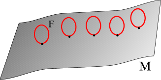
Figure 1: A noncommutative geometry can be pictured by imagining a Kaluza-Klein space where the compact extra dimensions $F$ are replaced by discrete matrix spaces $\mathcal{A}_{f}$ and space-time $M$ by the algebra of smooth functions $C^{\infty}(M)$ over $M$.

These product spaces the spectral triple approach, combined with the spectral action $\!{}^{{\bf?}}$, unify GR and the SM as classical field theories:

The SM in the NCG setting automatically produces:

• The combined GR and SM action

• A cosmological constant

• The Higgs boson with the correct quartic Higgs potential

The Dirac operator turns out to be one of the central objects and plays a multiple role:

2 Physical Consequences of the NCG formalism

Up to now one could conclude that NCG consists merely in a fancy, mathematically involved reformulation of the SM. But the choices of possible Yang-Mills-Higgs models that fit into the NCG framework is limited. Indeed the geometrical setup leads already to a set of restrictions on the possible particle models:

• mathematical axioms $=>$ restrictions on particle content

• symmetries of finite space $=>$ determines gauge group

• representation of matrix algebra $=>$ representation of gauge group

  (only fundamental and adjoint representations)

• Dirac operator $=>$ allowed mass terms / Higgs fields

Further constraints come from the Spectral Action which results in an effective action valid at a cut-off energy $\Lambda$ $\!{}^{{\bf?}}$. This effective action comes with a set of constraints on the standard model couplings, also valid at $\Lambda$, which reduce the number of free parameters in a significant way.

The Spectral Action contains two parts. A fermionic part $(\Psi,\mathcal{D}\Psi)$ which is obtained by inserting the Dirac operator into the scalar product of the Hilbert space and a bosonic part $S_{\mathcal{D}}(\Lambda)$ which is just the number of eigenvalues of the Dirac operator up to the cut-off:

• $(\Psi,\mathcal{D}\Psi)$ = fermionic action includes Yukawa couplings & fermion–gauge boson interactions

• $S_{\mathcal{D}}(\Lambda)$ = the bosonic action given by the number of eigenvalues of $\mathcal{D}$ up to cut-off $\Lambda$

  = the Einstein-Hilbert action + a Cosmological Constant

  + the full bosonic SM action + constraints at $\Lambda$

The bosonic action $S_{\mathcal{D}}(\Lambda)$ can be calculated explicitly using the well known heat kernel expansion $\!{}^{{\bf?}}$. Note that $S_{\mathcal{D}}(\Lambda)$ is manifestly gauge invariant and also invariant under the diffeomorphisms of the underlying space-time manifold.

For the SM the internal space is taken to be the matrix algebra $\mathcal{A}_{f}=\mathbb{C}\oplus M_{2}(\mathbb{C})\oplus M_{3}(\mathbb{C})\oplus\mathbb{C}$. The symmetry group of this discrete space is given by the group of (non-abelian) unitaries of $\mathcal{A}_{f}$: $U(2)\times U(3)$. This leads, when properly lifted to the Hilbert space, to the SM gauge group $U(1)_{Y}\times SU(2)_{w}\times SU(3)_{c}$. It is a remarkable fact that the SM fits so well into the NCG framework!

Calculating from the geometrical data the Spectral Action leads to the following constraints on the SM parameters at the cut-off $\Lambda$

$$g_{2}^{2}=\,g_{3}^{2}=\,\frac{Y_{2}^{2}}{H}\,\frac{\lambda}{24}\,=\,\frac{1}{4}\,Y_{2}$$ (3)

Where $g_{2}$ and $g_{3}$ are the $SU(2)_{w}$ and $SU(3)_{c}$ gauge couplings, $\lambda$ is the quartic Higgs coupling, $Y_{2}$ is the sum of all Yukawa couplings squared and $H$ is the sum of all Yukawa couplings to the fourth power.

Assuming the Big Desert and the stability of the theory under the flow of the renormalisation group equations we can deduce that $g_{2}^{2}(\Lambda)=g_{3}^{2}(\Lambda)$ at $\Lambda=1.1\times 10^{17}$ GeV (where we used the experimental values $g_{2}(m_{Z})=0.6514$, $\;g_{3}(m_{Z})=1.221$). Having thus fixed the cut-off scale $\Lambda$ we can use the remaining constraints to determine the low-energy value of the quartic Higgs coupling and the top quark Yukawa coupling (assuming that it dominates all Yukawa couplings). This leads to the following conclusions:

• $m_{\rm Higgs}=168.3\pm 2.5$ GeV

• $m_{\rm top}<190$ GeV

• no $4^{th}$ SM generation

Note that the prediction for the Higgs mass is already problematic in the light of recent data from the Tevatron $\!{}^{{\bf?}}$. Thus it seems plausible to consider also models beyond the SM. We will present one recently discovered model which may have an interesting phenomenology.

3 Beyond the Standard Model

The general strategy to find models beyond the SM within the NCG framework can be summarised as follows:

• find a finite geometry that has the SM as a sub-model (tricky)

  $=>$ particle content, gauge group & representation

• (make sure everything is anomaly free)

• compute the spectral action $=>$ constraints on the parameters at $\Lambda$

• determine the cut-off scale $\Lambda$ with suitable sub-set of the constraints

• use renorm. group equations to obtain the low energy values of interesting parameters

• check with experiment!

This general strategy led, among other models $\!{}^{{\bf?}}$, to the following extension of the SM $\!{}^{{\bf?}}$: The model contains in addition to the SM particles a new scalar field and a new fermion singlet in each generation. These particles are neutral with respect to the SM gauge group but charged under a new $U(1)_{X}$ gauge group under which in turn the SM particles are neutral.

The discrete space is a slight extension of the SM space, $\mathcal{A}_{f}=\mathbb{C}\oplus M_{2}(\mathbb{C})\oplus M_{3}(\mathbb{C})\oplus\mathbb{C}\oplus\mathbb{C}\oplus\mathbb{C}$, which results in a $U(1)$ extension of the SM gauge group: $G=U(1)_{Y}\times SU(2)_{w}\times SU(3)_{c}\times U(1)_{X}$. The new fermions carry a $U(1)_{X}$ charge which is vector-like (we call them $X$-particles), with masses $M_{X}\sim\Lambda$. Note that very similar models have been considered before $\!{}^{{\bf?}}$. The new scalar $\varphi$ also transforms under $U(1)_{X}$ and couples to the SM Higgs field $H$:

$$V_{\rm scalar}=-\mu_{1}^{2}|H|^{2}+\frac{\lambda_{1}}{6}\,|H|^{4}-\mu_{2}^{2}|\varphi|^{2}+\frac{\lambda_{2}}{6}\,|\varphi|^{4}+\frac{\lambda_{3}}{3}\,|H|^{2}|\varphi|^{2}$$ (4)

This Lagrangian leads to the following symmetry breaking pattern for the model:

$$U(1)_{Y}\times SU(2)_{w}\times SU(3)_{c}\times U(1)_{X}\rightarrow U(1)_{el.}\times SU(3)_{c}.$$ (5)

For the $X$-particles and for the $U(1)_{X}$ gauge bosons one finds the standard Lagrangian:

$$\mathcal{L}_{\rm ferm+gauge}=\bar{X}_{L}M_{X}X_{R}+g_{\nu,X}\bar{\nu}_{R}\varphi X_{L}+\ h.c.\ +\frac{1}{g_{4}^{2}}F^{\mu\nu}_{X}F_{X,\mu\nu}$$ (6)

Calculating the Spectral Action leads to a set of constraints very similar to the SM constraints,

$$g_{2}^{2}=g_{3}^{2}=\frac{\lambda_{1}}{24}\frac{(3g_{t}^{2}+g_{\nu}^{2})^{2}}{3g_{t}^{4}+g_{\nu}^{4}}=\frac{\lambda_{2}}{24}=\frac{\lambda_{3}}{24}\frac{3g_{t}^{2}+g_{\nu}^{2}}{g_{\nu}^{2}}\frac{1}{4}\,(3g_{t}^{2}+g_{\nu}^{2}),$$ (7)

where for the sake of simplicity we have only kept the top quark Yukawa coupling $g_{t}$ and the $\tau$-neutrino Yukawa coupling $g_{\nu}$. The latter can be of order one and leads via the seesaw mechanism to a small neutrino mass. The relevant free parameters in this model are the vacuum expectation value $|\langle\varphi\rangle|$ of the new scalar field $\varphi$ and the $U(1)_{X}$ gauge coupling $g_{4}$ at given energy (for example at the $Z$-mass).

One notes that the potential $V_{\rm scalar}$ of the scalar sector has a non-trivial minimum. But the vacuum expectation values of the new scalar $\varphi$ and the Higgs $H$ do no longer constitute the mass eigenvalues. The physical scalar fields mix, thus leading to a dependence of the mass eigenvalues on the vacuum expectation value of the new scalar, $|\langle\varphi\rangle|$. The vacuum expectation value of the SM Higgs field is still dictated by the $W$-boson mass.

Two examples of the dependence of the mass eigenvalues on $|\langle\varphi\rangle|$ are depicted in Fig. 2, for the exemplary values of the $U(1)_{X}$ gauge coupling, $g_{4}(m_{Z})=0.3$ (left figure) and $g_{4}(m_{Z})=0.7$ (right figure). For a detailed analysis of this model we refer to $\!{}^{{\bf?}}$.

\psfrag{AA}[Bl][l][0.4][0]{ $v_{2}/$ GeV}\psfrag{BB}[l][0.4][90]{ $m/$ GeV}\includegraphics[scale={0.4}]{massg403.eps}

\psfrag{AA}[Bl][l][0.4][0]{ $v_{2}/$ GeV}\psfrag{BB}[l][0.4][90]{ $m/$ GeV}\psfrag{AA}[Bl][l][0.4][0]{ $v_{2}/$ GeV}\psfrag{BB}[l][0.4][90]{ $m/$ GeV}\includegraphics[scale={0.4}]{massg407.eps}

Figure 2: Mass eigenvalues of the scalar fields in dependence of $v_{2}=\sqrt{2}\,|\langle\varphi\rangle|$. For the $U(1)_{X}$ gauge coupling we choose $g_{4}(m_{Z})=0.3$ (left) and $g_{4}(m_{Z})=0.7$ (right). From the $W$-mass follows $\sqrt{2}|\langle H\rangle|=246$ GeV.

4 Outlook

We conclude this paper with a “to-do-list” of some open questions that are worth to be addressed in the future:

• Full classification of models beyond the SM in NCG (LHC signature and/or dark matter?)

• Mechanisms for Neutrino masses (Dirac/Majorana masses or something different?)

• Renormalisation group flow for all couplings in the spectral action (Exact Renorm Groups, M. Reuter et al.)

• Spectral triples with Lorentzian signature (A. Rennie, M. Paschke, R. Verch,…)

References

References

- [1] A.H. Chamseddine and A. Connes, Commun. Math. Phys. 186, 731 (1997), A.H. Chamseddine, A. Connes and M. Marcolli, Adv. Theor. Math. Phys. 11, 911 (2007)
- [2] A. Connes, Noncommutative Geometry Academic Press , (1994), A. Connes and M. Marcolli Noncommutative Geometry, Quantum Fields and Motives AMS Colloquium Publications 55, (2008)
- [3] Tevatron New Phenomena, Higgs working group, for the CDF collaboration, DZero collaboration, Combined CDF and DZero Upper Limits on Standard Model Higgs-Boson Production with up to 4.2 fb-1 of Data, arXiv:0903.4001 [hep-ex] FERMILAB-PUB-09-060-E (2009)
- [4] C.A. Stephan, J. Phys. A 39, 9657 (2006), J.Phys. A 40, 9941 (2007), R. Squellari and C.A. Stephan, J.Phys. A 40, 10685 (2007)
- [5] C. A. Stephan, Phys. Rev. D 79, 065013 (2009)
- [6] J.J. van der Bij, Phys.Lett. B 56, 636 (2006), C.P. Burgess, M. Pospelov and T. ter Veldhuis Nucl.Phys. B 709, 619 (2001), V. Barger, P. Langacker, M. McCaskey, M. Ramsey-Musolf and G. Shaughnessy Phys.Rev. D 79, 015018 (2009)