Line shapes of optical Feshbach resonances near the intercombination transition of bosonic Ytterbium

Abstract

The properties of bosonic Ytterbium photoassociation spectra near the intercombination transition ${}^{1}S_{0}$–${}^{3}P_{1}$ are studied theoretically at ultra low temperatures. We demonstrate how the shapes and intensities of rotational components of optical Feshbach resonances are affected by mass tuning of the scattering properties of the two colliding ground state atoms. Particular attention is given to the relationship between the magnitude of the scattering length and the occurrence of shape resonances in higher partial waves of the van der Waals system. We develop a mass scaled model of the excited state potential that represents the experimental data for different isotopes. The shape of the rotational photoassociation spectrum for various bosonic Yb isotopes can be qualitatively different.

I Introduction

The properties of intercombination transitions in alkaline earth atoms and atoms with similar electronic structure has become an object of a growing number of experimental and theoretical studies. It is mostly caused by a variety of new applications in the physics of ultra cold atoms: from laser cooling and trapping ido03 ; curtis03 ; loftus04 to optical frequency standards wilpers02 ; barber06 ; letargat06 ; boyd07 .

Great progress in this area has been achieved for Ytterbium (Yb), which has 7 stable isotopes with atomic weights 168, 170, 171, 172, 173, 174, and 176. Quantum degenerate gases have been obtained for the bosonic isotopes ${}^{174}\rm{Yb}$ takasu03 , ${}^{170}\rm{Yb}$ fukuhara07a , and ${}^{176}\rm{Yb}$ fukuhara09 , and the fermionic isotopes ${}^{171}\rm{Yb}$ and ${}^{173}\rm{Yb}$fukuhara07b . Photoassociation spectroscopy has been carried out for bosons takasuPA ; tojo06 as well as fermions enomoto08 . A two-color photoassociation experiment has allowed a precise determination of the ground state s-wave scattering lengths for all combinations of Yb isotopes kitagawa08 . Finally, it was demonstrated that the significant change of the scattering properties for colliding ground state atoms can be achieved with optical Feshbach resonances in these systems enomoto08ofr .

This work is devoted to the theoretical study of the photoassociation spectra near the intercombination transition ${}^{1}S_{0}$–${}^{3}P_{1}$ of Yb for bosonic isotopes. We take advantage of the experimental photoassociation spectra for ${}^{174}\rm{Yb}_{2}$ and ${}^{176}\rm{Yb_{2}}$ from Tojo et al. tojo06 to precisely determine the binding energies of excited state molecular energy levels. In addition, we report new measurements of the binding energies of excited ${}^{170}\rm{Yb}_{2}$ and ${}^{172}\rm{Yb}_{2}$. Analysis of the photoassociation spectra also requires knowledge of the scattering properties in the ground electronic state of two colliding atoms. The necessary information and experimental data for all ground state isotopic combinations can be found in Ref. kitagawa08 .

Yb is an excellent example of a system for which the scattering properties can be easily tuned by the change of the isotopic combination, thus changing the reduced mass of the colliding pair. Such mass tuning of the scattering properties can also be very useful in other similar species with several isotopes. Development in the laser trapping and cooling of atoms such as Cd brickman07 and Hg walthe07 ; hachisu08 will hopefully allow photoassociation investigations of these systems in the future. Cadmium and Hg, like Yb, are good candidates for mass tuning of the scattering length because of their numerous isotopes. In addition, Hg is seen as a very promising candidate for future optical frequency standards. The clock frequency shift induced by black body radiation is especially small in Hg hachisu08 , compared with other Group II elements porsev06 .

II Photoassociation resonance

The two-body loss rate coefficient $K(\Delta;I,T)$ in the photoassociation process for a thermal cloud of ultracold atoms at temperature $T$ needs to be evaluated as an average over all possible momenta of two colliding atoms. This loss rate is directly dependent on the light intensity $I$ leading to the photoassociation as well as on the detuning of the light from the atomic resonance $\Delta$ and detuning $\Delta_{e}$ corresponding to the optical resonance coupling the scattering ground state ”$g$” with the excited ”$e$” bound state weiner99 .

The averaged loss rate can be written as ciurylo04 :

$$K(\Delta;I,T)=\left<{\cal K}(\Delta;I,\vec{p}_{c},\vec{p}_{r})\right>_{\vec{p}_{c},\vec{p}_{r}}\,,$$ (1)

where

$${\cal K}(\Delta;I,\vec{p}_{c},\vec{p}_{r})=\frac{\hbar\pi}{k_{r}\mu}\sum_{e,g}(2J_{g}+1)\frac{\Gamma_{pe}\Gamma_{eg}(I,\varepsilon_{r})}{[\Delta+\varepsilon_{D}+\varepsilon_{r}-\Delta_{e}-E_{e}(I,\varepsilon_{r})-E_{\rm rec,mol}]^{2}+[\Gamma_{e}(I,\varepsilon_{r})/2]^{2}}$$ (2)

is the loss rate napolitano94 ; julienne96 ; bohn99 corresponding to particular momentum vectors of the relative motion of the two colliding atoms $\vec{p}_{r}$ as well as the motion of their center of mass $\vec{p}_{c}$. Contributions from all possible transitions between excited bound and ground scattering states are included in this expression. They are taken in the sum with weights dependent on the total angular momentum $J_{g}$ of the two-atom system. In Eq. (2) the magnitude of the wave vector corresponding to the relative motion is $k_{r}=p_{r}/\hbar$, the kinetic energy of relative motion is $\varepsilon_{r}={\hbar}^{2}k_{r}^{2}/(2\mu)$, and $\mu$ is the reduced mass of the colliding atoms. The Doppler shift is described by $\varepsilon_{D}=-\hbar\vec{k}_{\rm las}\cdot\vec{p}_{c}/{\cal M}$ where the magnitude of the laser light wave vector is $k_{\rm las}=\omega/c$ and the mass of the molecule created in the photoassociation process is ${\cal M}$. The shift of the photoassociation resonance $E_{\rm rec,mol}=\hbar^{2}k_{las}^{2}/(2{\cal M})$ caused by the photon recoil is also included here. Finally, the light induced shift of a given photoassociation resonance can be expressed as a sum $E_{e}(I,\varepsilon_{r})=\sum_{g}E_{eg}(I,\varepsilon_{r})$ of contributions $E_{eg}(I,\varepsilon_{r})$ of all possible optical transitions between the excited bound state ”$e$” and ground scattering states ”$g$”. Similarly, the total width of the resonance $\Gamma_{e}(I,\varepsilon_{r})=\Gamma_{pe}+\sum_{g}\Gamma_{eg}(I,\varepsilon_{r})$, where $\Gamma_{eg}(I,\varepsilon_{r})$ is the light induced width between the ”$e$” and ”$g$” states and $\Gamma_{pe}$ describes all possible other processes leading to loss of the excited state. If radiative decay is the dominant loss process, then $\Gamma_{pe}$ can be taken as the natural width of the excited molecular state.

The light induced width napolitano94 ; julienne96 ; bohn99

$$\Gamma_{eg}(I,\varepsilon_{r})=2\pi\left|\left<\Psi_{e}\right|V_{\rm las}(I)\left|\Psi_{g}^{+}(\varepsilon_{r})\right>\right|^{2}$$ (3)

is linearly dependent on the light intensity $I$ through the operator $V_{\rm las}(I)$ describing optical coupling between particular excited and ground states. For the case investigated here more details about this operator can be found in Refs. ciurylo04 ; napolitano97 . This width also depends on the kinetic energy of the relative motion of the two colliding atoms $\varepsilon_{r}$. This is because the energy normalized ground scattering state $\left|\Psi_{g}^{+}(\varepsilon_{r})\right>$ strongly depends on this energy. Finally the magnitude of the light-induced width is dependent on the unit normalized excited bound state $\left|\Psi_{e}\right>$.

The light induced shift bohn99 can be calculated from the Fano theory fano61 ; simoni02

$$E_{eg}(I,\varepsilon_{r}) = \frac{1}{2\pi}{\cal P}\int_{0}^{\infty}d\varepsilon\frac{\Gamma_{eg}(I,\varepsilon_{r})}{\varepsilon_{r}-\varepsilon}$$ (4)

$$+\sum_{\left|\Psi_{g}\right>}\frac{\left|\left<\Psi_{e}\right|V_{\rm las}(I)\left|\Psi_{g}\right>\right|^{2}}{\varepsilon_{r}-E_{g}}\,,$$

where ${\cal P}$ is a principal part integral over all collision energies, and the sum occurring in this expression is taken over all unity normalized bound state $\left|\Psi_{g}\right>$ of the ground electronic potential. Like in the case of the light induced width, the light induced shift is linearly dependent on the laser intensity $I$ and of course on $\varepsilon_{r}$.

The photoassociation process can be viewed as a case of the optical Feshbach resonance bohn99 ; fedichev96 ; bohn97 . The optical coupling of the ground scattering state to the excited bound state changes both the amplitude and the phase of the scattering wave function. The amplitude can be detected through loss of atoms from the trap. The phase change can also be detected fatemi00 ; enomoto08ofr . This approach leads to conclusion that the scattering length describing ultra cold collisions of the two ground state atoms can be modified by light due to the coupling with an excited bound state. This effect was demonstrated with a Bose-Einstein condensate (BEC) of ⁸⁷Rb theis04 ; thalhammer05 . The expression for a scattering length modified by light can be written in the following form bohn99 :

$$a(\Delta,I)=a_{\rm bg}+\sum_{e}l_{eg}^{\rm opt}(I,0)\frac{\Gamma_{pe}[\Delta-\Delta_{e}-E_{e}(I,0)-E_{\rm rec,mol}]}{[\Delta-\Delta_{e}-E_{e}(I,0)-E_{\rm rec,mol}]^{2}+[\Gamma_{e}(I,0)/2]^{2}}\,,$$ (5)

where $a_{\rm bg}$ is the background scattering length of the system in absence of the light. The optical length $l_{eg}^{\rm opt}(I,\varepsilon_{r})$ bohn97 ; ciurylo05 is

$$l_{eg}^{\rm opt}(I,\varepsilon_{r})=\frac{\Gamma_{eg}(I,\varepsilon_{r})}{2k_{r}\Gamma_{pe}}\,.$$ (6)

Because of the $s$-wave threshold law, this quantity approaches an energy-independent constant as $\varepsilon_{r}\to 0$ that varies linearly with light intensity $I$. The optical length characterizes the strength of an optical Feshbach resonance, namely the ability of light to change the scattering length of the ground state atoms; see also Ref. chin08 for a review of Feshbach resonances, including optical ones. The scattering length can be changed on the order of its background magnitude $|a_{\rm bg}|$ while minimizing losses if the optical length is very large compared with $|a_{\rm bg}|$ so that the optical control can be achieved at large detuning.

III Derivation of a single channel model

The particular properties of the photoassociation resonances are strongly dependent on the properties of the atomic interaction of the colliding atoms. In general we describe the colliding system using the Hamiltonian operator $H=T+H_{A}+V_{\rm int}+V_{\rm rot}$. In this expression $T$ is the kinetic energy operator for relative radial motion, $H_{A}$ is the atomic Hamiltonian operator representing internal atomic degrees of freedom, $V_{\rm int}$ is the interaction operator described by nonrelativistic molecular Born-Oppenheimer potentials, and $V_{\rm rot}$ is the rotational energy operator. Reference ciurylo04 gives more details for the case investigated here.

Let us first focus on the interaction in the excited state. In this paper we limit our discussion to photoassociation near the intercombination transition ${}^{1}S_{0}$–${}^{3}P_{1}$. Therefore we will discuss the atomic interaction properties only near the dissociation limit ${}^{1}S_{0}+^{3}P_{1}$. In this case it is convenient to use the $|jlJM;p\rangle$ basis. Here $\vec{j}$ is the total electron angular momentum, $\vec{l}$ is the rotational angular momentum, and $\vec{J}=\vec{j}+\vec{l}$ is the total angular momentum. The projections of $\vec{J}$ on a space-fixed $z$ axis is $M$. Finally $p$ is the total parity. We add an index $e$ to all quantities introduced here to indicate that they correspond to the excited electronic state. It should be noted that $J_{e}$ as well as $M_{e}$ are good quantum numbers of the Hamiltonian $H$. In our case with $j_{e}=1$ and $p_{e}=-1$ we can solve the Schrödinger equation using only two channels for each $J_{e}$: one with $l_{e}=J_{e}-1$ and one with $l_{e}=J_{e}+1$. In this basis the interaction operator $V_{\rm int}$ is not diagonal. Its matrix elements can be expressed in terms of potentials $V_{0}(r)$ and $V_{1}(r)$ which correspond to states with $\Omega=0$ and $\Omega=1$, respectively, where $\Omega$ is the projection of the total electron angular momentum $j_{e}$ along the interatomic axis. The other components of the Hamiltonian operator, $T$, $H_{A}$, and $V_{\rm rot}$, are diagonal in our basis.

The matrix elements of the sum $V_{\rm int}+V_{\rm rot}$ can be written in a compact form julienne86 :

$$\begin{array}[]{c}\begin{array}[]{cc}l_{e}=J_{e}-1&l_{e}=J_{e}+1\vspace{3mm}\end{array}\\ \left(\begin{array}[]{cc}\frac{J_{e}}{2J_{e}+1}V_{0}(r)+\frac{J_{e}+1}{2J_{e}+1}V_{1}(r)+B(r)J_{e}(J_{e}-1)&\frac{\sqrt{J_{e}(J_{e}+1)}}{2J_{e}+1}[V_{1}(r)-V_{0}(r)]\\ \frac{\sqrt{J_{e}(J_{e}+1)}}{2J_{e}+1}[V_{1}(r)-V_{0}(r)]&\frac{J_{e}+1}{2J_{e}+1}V_{0}(r)+\frac{J_{e}}{2J_{e}+1}V_{1}(r)+B(r)(J_{e}+2)(J_{e}+1)\\ \end{array}\right)\end{array}\begin{array}[]{c}\vspace{3mm}\hfil\\ \vspace{3mm}l_{e}=J_{e}-1\vspace{3mm}\\ l_{e}=J_{e}+1\end{array}$$ (7)

where $B(r)=\hbar^{2}/(2\mu r^{2})$. Henceforth we will omit explicit indication of the $r$-dependence of $V_{0}$, $V_{1}$ and $B$. Analytic diagonalization of this matrix gives the following eigenvalues:

$${\cal V}_{0} = \frac{1}{2}\left\{V_{0}+V_{1}-(V_{1}-V_{0})\sqrt{1-\frac{4B}{V_{1}-V_{0}}+\frac{4B^{2}(2J_{e}+1)^{2}}{(V_{1}-V_{0})^{2}}}+2B[J_{e}(J_{e}+1)+1]\right\}\,,$$ (8)

$${\cal V}_{1} = \frac{1}{2}\left\{V_{0}+V_{1}+(V_{1}-V_{0})\sqrt{1-\frac{4B}{V_{1}-V_{0}}+\frac{4B^{2}(2J_{e}+1)^{2}}{(V_{1}-V_{0})^{2}}}+2B[J_{e}(J_{e}+1)+1]\right\}\,.$$ (9)

These eigenvalues ${\cal V}_{0}$ and ${\cal V}_{1}$ can be used as effective potentials for single channel calculations of excited bound states. Such an approach allows one to approximate the influence of Coriolis coupling on the molecular structure in simple single channel calculations.

The quantum number $\Omega$ becomes a good one in the range of $r$ where $\left|V_{1}-V_{0}\right|\gg B$, i e., when the anisotropy of the interaction between two atoms is much bigger than the rotation energy. In such a case the eigenvalues and corresponding eigenvectors of the matrix in Eq. (7) can be written in the following form:

$${\cal V}_{0} = V_{0}+B[J_{e}(J_{e}+1)+2]\longrightarrow\left(\begin{array}[]{c}-\sqrt{J_{e}/(2J_{e}+1)}\vspace{3mm}\\ \sqrt{(J_{e}+1)/(2J_{e}+1)}\end{array}\right)\,,$$ (12)

$${\cal V}_{1} = V_{1}+BJ_{e}(J_{e}+1)\hskip 22.76219pt\longrightarrow\left(\begin{array}[]{c}\sqrt{(J_{e}+1)/(2J_{e}+1)}\vspace{3mm}\\ \sqrt{J_{e}/(2J_{e}+1)}\end{array}\right)\,.$$ (15)

In many cases these potentials provide a successful approximation for single channel calculations of bound states of real systems. Such an approach is particularly good for Yb, because the potential curves at long range are dominated by the resonant dipole interaction. In the case of Yb $\left|V_{1}-V_{0}\right|=\frac{3}{2}C_{3}/r^{3}\gg B$ up to very large $r$. This is a quite different case from Sr zelevinsky06 , where the $C_{3}$ value is more than 20 times smaller than for Yb. In the case of Sr the competition between the van der Waals and resonance interactions is important. In the range of $r$ where the interaction is dominated by the resonant dipole term the ungerade potentials for $\Omega=0$ and $\Omega=1$ are attractive and repulsive, respectively. Therefore only the potential ${\cal V}_{0}$ will support a series of bound states having $0_{u}^{+}$ symmetry near the dissociation limit. The ${\cal V}_{1}$ potential becomes attractive at small $r$ due to chemical bonding and may support a bound state near the dissociation limit. In the rest of the paper we will describe excited bound states of $0_{u}^{+}$ symmetry using single channel solutions of the Schrödinger equation.

This simple approach to the description of atomic interactions allows us to write the appropriate expressions for the light induced width and shift:

$$\Gamma_{eg}(I,\varepsilon_{r})=\Gamma_{A}\frac{3}{4\pi}\frac{I\lambda_{A}^{3}}{c}f_{eg}^{\rm rot}f_{eg}^{\rm FC-\Gamma}(\varepsilon_{r})$$ (16)

and

$$E_{eg}(I,\varepsilon_{r})=\Gamma_{A}\frac{3}{4\pi}\frac{I\lambda_{A}^{3}}{c}f_{eg}^{\rm rot}f_{eg}^{\rm FC-E}(\varepsilon_{r})\,.$$ (17)

In Eqs. (16) and (17) $\Gamma_{A}$ is the natural decay width of the atomic transition and $\lambda_{A}$ the wavelength of the atomic transition. The dimensionless rotational line strength factor for a transition from the ground scattering state to the excited $0_{u}^{+}$ state in a bosonic isotope has the simple approximate form obtained by Machholm et al. machholm01 :

$$f_{eg}^{\rm rot}=\left\{\begin{array}[]{cc}\frac{1}{3}\frac{2J_{e}+1}{2J_{g}+1}\frac{J_{e}}{2J_{e}+1}=\frac{1}{3}\frac{J_{g}+1}{2J_{g}+1}&\mbox{for $J_{e}=J_{g}+1$}\vspace{3mm}\,,\\ \frac{1}{3}\frac{2J_{e}+1}{2J_{g}+1}\frac{J_{e}+1}{2J_{e}+1}=\frac{1}{3}\frac{J_{g}}{2J_{g}+1}&\mbox{for $J_{e}=J_{g}-1$}\,.\end{array}\right.$$ (18)

for even $J_{g}$. This expression can be obtained using the approach described in Ref. ciurylo04 . To extract the rotational line strength factor $f_{eg}^{\rm rot}$ one can start from Eq. (3) and use Eq. (B3) from Ref. ciurylo04 . In our case, this allows us to show that the laser radiation couples the ground scattering channel having $l_{g}=J_{g}$ only with the excited state channel having the same $l_{e}$. Therefore the light induced width, Eq. (3), is proportional to the fraction of the total wave function of the excited bound state in the channel with $l_{e}=l_{g}$. This fraction can be found from Eqs. (12) and (15). Moreover, the light induce width is proportional to the square of the proper Clebsch-Gordan coefficient $\left|\left<J_{g}KM_{g}q|J_{e}M_{e}\right>\right|$, where $K=1$ for the dipole transition and $q=-1,\;0,\;{\rm or}\;+1$ describes the polarization of light. This way one can introduce the rotational line strength factor

$$f_{eg}^{\rm rot}(M_{g},q)=\frac{2J_{g}+1}{2J_{e}+1}\left|\left<J_{g}100|J_{e}0\right>\right|^{2}\left|\left<J_{g}KM_{g}q|J_{e}M_{e}\right>\right|^{2},$$ (19)

which is dependent on the light polarization $q$ and the projection $M_{g}$ of the total angular momentum $J_{g}$ in the ground electronic state, see Ref. vogt07 .

The rotational line strength factor given by Eq. (18) can be obtained as an average

$$f_{eg}^{\rm rot}=\frac{1}{2J_{g}+1}\sum_{M_{g}}f_{eg}^{\rm rot}(M_{g},q)$$ (20)

over all possible orientations of the total angular momentum $J_{g}$; compare Refs. machholm01 ; vogt07 . This quantity is independent of the light polarization $q$. To derive Eq. (18) one can use the following relation

$$\sum_{M_{g}}\left|\left<J_{g}KM_{g}q|J_{e}M_{e}\right>\right|^{2}=\frac{2J_{e}+1}{3}\;,$$ (21)

which is fulfilled for $J_{e}=J_{g}-1\;{\rm and}\;J_{g}+1$, $K=1$ and $M_{e}=M_{g}+q$. Equation (18) can be also expressed in terms of a Wigner 3-$j$ symbol, see Ref. vogt07 :

$$f_{eg}^{\rm rot}=\frac{\left|\left<J_{g}100|J_{e}0\right>\right|^{2}}{3}=\frac{2J_{e}+1}{3}\left(\begin{array}[]{ccc}J_{g}&1&J_{e}\\ 0&0&0\end{array}\right)^{2}.$$ (22)

This work is limited only to the case of weak interaction with light. Therefore we can ignore the dependence of the light induced width and shift on the projection $M_{g}$ and use the projection independent Eq. (18).

The total angular momentum $J_{g}$ in the ground scattering state is the same as the rotational angular momentum $l_{g}$. This is a consequence of the fact that the atomic interaction in the ground electronic state has ${}^{1}\Sigma_{g}^{+}$ symmetry and the total electronic angular momentum $j_{g}=0$. In homonuclear pairs of bosonic atoms only even $J_{g}$ are allowed. Finally, the Franck-Condon factors bohn99 :

$$f_{eg}^{\rm FC-\Gamma}(\varepsilon_{r})=\left|\int_{0}^{\infty}dr\;\phi_{e}(r)f_{g}(r;\varepsilon_{r})\right|^{2}$$ (23)

and

$$f_{eg}^{\rm FC-E}(\varepsilon_{r})=\int_{0}^{\infty}dr\;\phi_{e}(r)g_{g}(r;\varepsilon_{r})\int_{0}^{r}dr^{\prime}\phi_{e}(r^{\prime})f_{g}(r^{\prime};\varepsilon_{r})$$ (24)

can be expressed in terms of the regular $f_{g}(r;\varepsilon_{r})$ and irregular $g_{g}(r;\varepsilon_{r})$ solutions of the the Schrödinger equation for the ground scattering state and the wave function $\phi_{e}(r)$ for the excited bound state.

The expressions for the light induced width and shift can be further simplified by using the reflection approximation bohn99 ; julienne96 ; boisseau00b . The Franck-Condon factors can then be written in the following form:

$$f_{eg}^{\rm FC-\Gamma}(\varepsilon_{r})=\frac{\partial E_{e}}{\partial n}\frac{1}{D_{C}}\left|f_{g}(r_{C};\varepsilon_{r})\right|^{2}$$ (25)

and

$$f_{eg}^{\rm FC-E}(\varepsilon_{r})=\frac{1}{2}\frac{\partial E_{e}}{\partial n}\frac{1}{D_{C}}g_{g}(r_{C};\varepsilon_{r})f_{g}(r_{C};\varepsilon_{r})\,.$$ (26)

where $D_{C}=\left.\partial{\cal V}_{e}/\partial r\right|_{r_{C}}-\left.\partial{\cal V}_{g}/\partial r\right|_{r_{C}}$ the fraction $\frac{\partial E_{e}}{\partial n}$ is the mean vibrational spacing, ${\cal V}_{e}$ and ${\cal V}_{g}$ are the effective potentials in the excited and ground electronic states. Here $r_{C}$ is the Condon point. When the reflection approximation is applicable, the Condon point is approximately the classical outer turning point for the excited bound state.

The reflection approximation is very good for a number of Yb bound states close to the ${}^{1}S_{0}+^{3}P_{1}$ dissociation limit. This is in contrast with other species such as Ca or Sr, for which the reflection approximation needs to be modified ciurylo06 . Since Eqs. (16) and (25) show that the light induced width is proportional to $|f_{g}(r_{C})|^{2}$, photoassociation spectroscopy provides an excellent tool to investigate the properties of the ground state scattering wave function jones06 . This will be explored below for photoassociation of Yb near the intercombination line.

IV Experimental data

Experimental information is crucial for determining the parameters that describe the long range interaction near the ¹S₀–³P₁ dissociation limit. We used the experimental data obtained by Tojo et al. tojo06 to find the parameters needed to describe $V_{0}(r)$ for the $0_{u}^{+}$ state. As described in Ref. tojo06 , Yb atoms were decelerated by a Zeeman-slowing laser for the ¹S₀–¹P₁ transition, and were collected in a magneto-optical trap (MOT) with a laser for the ¹S₀–³P₁ transition. After the compression of the MOT, the atoms were transferred into a crossed optical trap with laser beams at 532 nm. The atoms were evaporatively cooled by decreasing the trap potential depth. Typically, MOT duration time is 10 s and evaporative cooling time is 6 s. A laser beam for photoassociation was applied to the trapped atoms, and the number of remaining atoms was measured through an absorption image with the ¹S₀–¹P₁ transition after the release from the optical trap. The applied photoassociation light intensity varied between 6.5 $\mu$W/cm² to 90 mW/cm², depending on which excited level was being probed. We obtained the atom-loss spectra by scanning the photoassociation laser frequency. These spectra allowed the determination of the bound states energies of a series of $J_{e}=1$ and $J_{e}=3$ $0_{u}^{+}$ levels for each of the two isotopic species. Table 1 lists the measured energies along with their error bars. The data for the ¹⁷⁴Yb₂ $J_{e}=1$ states were taken at about 4 $\mu$K, and the other data in Table 1 were taken at temperatures in the range from 5 to 27 $\mu$K. The shift with temperature and light intensity of the photoassociation features was taken into account in the data analysis. These shifts are mostly responsible for the magnitude of the error bars listed in Table 1.

Table 1: Comparison of measured binding energies in excited $0_{u}^{+}$ state for ${}^{174}{\rm Yb}_{2}$ and ${}^{176}{\rm Yb}_{2}$ with binding energies calculated from the optimal model obtained by least squares fit of experimental data for ${}^{174}{\rm Yb}_{2}$ and ${}^{176}{\rm Yb}_{2}$ isotopes. See details in the text. All quantities are given in MHz.

174Yb						176Yb
$J_{e}=1$			$J_{e}=3$			$J_{e}=1$			$J_{e}=3$
Experiment	Theory	Diff.	Experiment	Theory	Diff.	Experiment	Theory	Diff.	Experiment	Theory	Diff.
-4.4(1.0)	-4.2	-0.2		-3			-3.1			-2.1
-9.6(1.0)	-9.7	0.1		-7.5		-7.9(2.0)	-7.5	-0.4	-5.9(2.0)	-5.7	-0.2
-19.7(1.0)	-20.1	0.4	-16.1(2.0)	-16.7	0.6	-16.5(2.0)	-16.0	-0.5	-13.9(2.0)	-13.1	-0.8
-37.4(1.0)	-38.5	1.1	-32.5(2.0)	-33.3	0.8	-32.0(2.0)	-31.2	-0.8	-27.4(2.0)	-26.8	-0.6
-68.5(1.0)	-69.1	0.6		-61.7		-56.2(2.0)	-57.0	0.8	-50.0(2.0)	-50.5	0.5
-119.1(2.0)	-117.8	-1.3		-107.5			-98.5			-89.4
-191.3(1.0)	-192.3	1.0	-179.0(2.0)	-178.2	-0.8		-162.6			-150.1
-302.3(1.0)	-302.5	0.2	-284.5(2.0)	-283.9	-0.6	-258.2(2.0)	-258.3	0.1	-242.8(2.0)	-241.7	-1.1
-461.1(1.0)	-461.3	0.2		-437.4		-398.1(2.0)	-397.1	-1.0	-376.4(2.0)	-375.5	-0.9
-684.6(1.0)	-684.9	0.3	-654.7(2.0)	-654.6	-0.1	-594.4(2.0)	-593.8	-0.6	-567.3(2.0)	-566.3	-1.0
-993.7(1.0)	-993.7	0.0		-955.9		-867.6(2.0)	-866.7	-0.9	-832.7(2.0)	-832.2	-0.5
-1412.8(1.0)	-1413.0	0.2	-1366.7(2.0)	-1366.4	-0.3	-1240.1(2.0)	-1238.9	-1.2		-1196.2
-1973.5(1.0)	-1973.9	0.4	-1918.1(2.0)	-1917.3	-0.8		-1738.5			-1686.5

The same technique was used to determine bound states energies of the excited homonuclear molecules made from two other bosonic isotopes, ¹⁷⁰Yb and ¹⁷²Yb. Long MOT time of about 60 s was needed for ¹⁷⁰Yb because of its small natural abundance fukuhara07a , and the evaporative cooling had to be done in a short time of about 1.5 s for ¹⁷²Yb because of three-body recombination atom loss due to its large negative scattering length enomoto08ofr . Table 2 lists the values of measured binding energies in the excited $0_{u}^{+}$ $J_{e}=1$ levels of ${}^{170}{\rm Yb}_{2}$ and ${}^{172}{\rm Yb}_{2}$ molecules. These data were taken at about 2 $\mu$K. The uncertainties shown in Table II are mostly due to the light-induced shift.

Table 2: Comparison of measured binding energies in excited $0_{u}^{+}$ state for ${}^{170}{\rm Yb}_{2}$ and ${}^{172}{\rm Yb}_{2}$ with binding energies calculated from the optimal model obtained by least squares fit of experimental data for ${}^{174}{\rm Yb}_{2}$ and ${}^{176}{\rm Yb}_{2}$ isotopes. See details in the text. All quantities are given in MHz.

170Yb			172Yb
$J_{e}=1$			$J_{e}=1$
Experiment	Theory	Diff.	Experiment	Theory	Diff.
	-2.9			-2.2
	-7.2			-5.5
	-15.6			-12.4
	-31.0		-26.7(1.0)	-25.1	-1.6
	-57.3		-48.9(1.0)	-47.1	-1.8
	-99.9			-83.3
	-166.1		-142.6(5.0)	-140.2	-2.4
-268.1(3.0)	-265.4	-2.7	-228.7(1.0)	-226.4	-2.3
-412.9(3.0)	-410.4	-2.5	-355.3(1.0)	-352.9	-2.4
-619.3(3.0)	-616.6	-2.7	-544.1(5.0)	-534.1	-10
-906.3(3.0)	-903.9	-2.4	-798.1(5.0)	-787.9	-10.2
	-1296.9		-1145.1(5.0)	-1136.6	-8.5
	-1826.5			-1608.1

V Model potentials

The location of a photoassociation resonance as the laser frequency is scanned is directly related to the binding energy of the excited molecule. Ab initio potential curves are still insufficiently accurate to describe the position of the most weakly bound states. Therefore we introduce an analytic model potential valid at large $r$ and fit its parameters to match measured bound state energies near the dissociation limit for different isotopes. The basic concept is similar to that used very successfully for bound state and scattering properties of the ground state kitagawa08 ; vankempen02 . The potential is chosen to have the correct long range form and an arbitrary short range form that permits us to represent the correct absolute phase due to the unknown short range interactions. This allows us to successfully mass scale the excited state binding energies for different isotopic combinations. Mass scaling is more fully described in the next Section.

The interaction potential of two atoms in the $0_{u}^{+}$ excited electronic state for large interatomic separations can be well approximated by the following expression (see Ref. zelevinsky06 ):

$$V_{0}(r)=\frac{C^{(e)}_{6}}{r^{6}}\left[\left(\frac{\sigma^{(e)}}{r}\right)^{6}-1\right]-\frac{C^{(e)}_{8}}{r^{8}}-\frac{C^{(e)}_{3}}{r^{3}}\,,$$ (27)

where the resonant dipole-dipole interaction coefficient

$$C^{(e)}_{3}=\frac{3}{2}\frac{\hbar}{\tau}\left(\frac{\lambda}{2\pi}\right)^{3}\,,$$ (28)

and $\sigma^{(e)}$ is a free parameter that allows us to adjust the phase associated with the short range potential. The wavelength of light in vacuum corresponding to the transition between atomic states ${}^{1}S_{0}$ and ${}^{3}P_{1}$ of Yb is $\lambda=555.802\;{\rm nm}$, and $\tau$ is the atomic lifetime. We use the least-squares method to optimize the values of $C^{(e)}_{3}$, $C^{(e)}_{6}$, $C^{(e)}_{8}$, and $\sigma^{(e)}$ while matching the calculated binding energies to the experimental values measured by Tojo et al. tojo06 for ${}^{174}{\rm Yb}$ and ${}^{176}{\rm Yb}$. We obtain $C_{3}^{(e)}=0.1949(11)\;E_{h}a_{0}^{3}$ which corresponds to $\tau=869.6(4.5)\;{\rm ns}$, $C^{(e)}_{6}=2.41(0.22)\times 10^{3}\;E_{h}a_{0}^{6}$, $C^{(e)}_{8}=2.3(1.6)\times 10^{5}\;E_{h}a_{0}^{8}$, and $\sigma^{(e)}=8.5(1.0)\;a_{0}$, where $a_{0}\approx 0.05292\;{\rm nm}$ and $E_{h}\approx 4.360\times 10^{-18}\;{\rm J}$. The errors quoted give the one standard deviation statistical fitting error, and do not reflect any systematic errors in the model. Adding the $C^{(e)}_{8}$ coefficient to the model was needed to improve the quality of the fit for $J_{e}=3$ levels. Introducing $C^{(e)}_{8}$ allowed us to determine the sensitivity of $C^{(e)}_{6}$ to variation of the shorter range of the potential. This sensitivity also contributes to the standard deviation of $C^{(e)}_{6}$. For completeness we give the fitting parameters to enough significant digits to reproduce the calculated values to 10 kHz, as shown in Table 1: $C^{(e)}_{3}=0.19488626\;E_{h}a_{0}^{3}$ ($\tau=869.64762\;{\rm ns}$), $C^{(e)}_{6}=2405.3647\;E_{h}a_{0}^{6}$, $C^{(e)}_{8}=229451.31\;E_{h}a_{0}^{8}$, and $\sigma^{(e)}=8.4897163\;a_{0}$.

Table 1 compares the binding energies predicted by the model to the experimental data for ${}^{174}\rm{Yb}_{2}$ and ${}^{176}\rm{Yb}_{2}$. The model predicts the experimental values to within about one MHz on the average, consistent with the experimental error bars.

Having the data for two different isotopes allows us to construct an appropriately mass-scaled model for the excited state levels, similar to what is possible for the ground state kitagawa08 . While cautioning that the short range physics is complicated by the interaction of other molecular states with the $0_{u}^{+}$ state and may not be fully represented by a single potential, our mass scaled model determines that the most deeply bound observed levels at $-1973.5$ MHz for ${}^{174}\rm{Yb}_{2}$ and $-1240$ MHz for ${}^{176}\rm{Yb}_{2}$ respectively correspond to the $v=$ 106 and 108 vibrational levels of the model potential.

An excellent test of mass scaling is to test it using other isotopic combinations. Table 2 shows a comparison of our new measured binding energies for ${}^{170}\rm{Yb}_{2}$ and ${}^{172}\rm{Yb}_{2}$ with those predicted by our mass scaled single-potential model. There is reasonable agreement of about 3 MHz between measured and calculated levels, except for the three most deeply bound levels observed for ${}^{172}\rm{Yb}_{2}$. While 3 MHz is on the order of the experimental uncertainty, the accuracy of mass scaling may be more limited for the excited states than for the ground states, where it was found to be good to approximately 0.1 MHz kitagawa08 for binding energies up to 325 MHz. Another source of error in our single channel excited state model could be the neglect of interactions with short range eigenstates of other symmetries. For example, it may be that bound states of $1_{u}$ symmetry near the threshold perturb the $0_{u}^{+}$ bound states that are near in energy to them. This could be the reason for relatively large deviations for the three most deeply bound states of ${}^{172}\rm{Yb}$.

Our model potential describing the interaction in the electronic excited state $0_{u}^{+}$ has a very different shape from those obtained in an ab initio calculation by Wang and Dolg wang98 . Clearly such a model can not be treated as a good representation of the short range interaction. Nevertheless, its applicability over a range of isotope masses gives us confidence that the number of bound states determined from our model is correct to within one or two bound states. The vibronic quantum number for the ${}^{174}\rm{Yb}$ bound state at -4.4 MHz is 118 with the ground state labeled as zero. Also the long range interaction should be well described by the model used here.

Table 3: Corrections to binding energies of the $0_{u}^{+}$ bound states with $J_{e}=1$ in the ${}^{174}{\rm Yb}_{2}$ molecule caused by the Coriolis coupling and retardation effect; see the text for details. All calculated values are given in MHz.

Binding	Corrections
Energy	Coriolis	Retardation 1	Retardation 2
-4.2	-0.004	-0.5	-0.5
-9.7	-0.005	-0.6	-0.6
-20.1	-0.006	-0.8	-0.7
-38.5	-0.008	-1.0	-0.9
-69.1	-0.009	-1.2	-1.0
-117.8	-0.011	-1.4	-1.1
-192.3	-0.013	-1.7	-1.2
-302.5	-0.015	-1.9	-1.2
-461.3	-0.017	-2.2	-1.2
-684.9	-0.020	-2.5	-1.1
-993.7	-0.022	-2.8	-0.9
-1413.0	-0.025	-3.1	-0.5
-1973.9	-0.027	-3.5	0.0

We have tested the possible influence of the Coriolis coupling on the results of our calculations. We have compared our calculation used for the fits in which effective potential was given by Eq. (12) with those obtained using the effective potential in the form of Eq. (8), and find only a small difference in binding energies for $0_{u}^{+}$ bound states with $J_{e}=1$ in the ${}^{174}{\rm Yb}_{2}$ molecule. Table 3 shows the magnitude of the Coriolis corrections in the column labeled ”Coriolis”. These corrections calculated from the single channel model, Eq. (8), are below 30 kHz and much less than the experimental error bars. The relative importance of this correction increases as the bound state energy approaches the threshold. The Coriolis coupling mostly play a marginal role in the Yb₂ excited state system. By contrast, Ref.  zelevinsky06 showed it needs to be taken into account to correctly calculate two most weakly bound $0_{u}^{+}$ states with $J_{e}=1$ in the ${}^{88}{\rm Sr}_{2}$ molecule.

Similar tests were carried out to check the possible influence of retardation effects power67 ; meath68 . To do this we have replaced in the effective potential, Eqs. (12) and (27), the standard term describing the resonance interaction $-C_{3}^{(e)}/r^{3}$ by the term in which retardation is taken into account: $-(C_{3}^{(e)}/r^{3})[\cos(r/\lambdabar)+(r/\lambdabar)\sin(r/\lambdabar)]$, where $\lambdabar=\lambda/(2\pi)$ meath68 ; machholm01 . The corrections to the binding energies caused by this change are listed in the column ”Retardation 1” of Table 3. These corrections are on the order of a few MHz. In contrast, the same corrections for ${}^{88}{\rm Sr}_{2}$ molecule zelevinsky06 are more than one order of magnitude smaller. To check whether such shifts might be detectable in fitting the data, we have modified $\sigma^{(e)}$ so as to change the quantum defect and fit the binding energy of the most bound level. The column labeled ”Retardation 2” show the differences from the values calculated without retardation. Since these differences are on the order of 1 MHz or less, comparable to the experimental uncertainty, the present data are not sufficiently accurate to come to any definitive conclusions about the observability of retardation corrections.

Table 4: Comparison of experimental ground state binding energies kitagawa08 with the present model. All values are given in MHz. The last column is the difference between the experimental values and the present model.

Isotope	v	$J_{g}$	Experiment	Theory	Theory	Diff.
			kitagawa08	kitagawa08	Present work
176Yb	1	0	-70.404	-70.405	-70.378	-0.026
	1	2	-37.142	-37.118	-37.093	-0.049
174Yb	1	0	-10.612	-10.642	-10.629	0.018
	2	0	-325.607	-325.607	-325.602	-0.005
	1	2	-268.575	-268.576	-268.570	-0.005
173Yb	1	0	-1.539	-1.613	-1.609	0.070
172Yb	1	0	-123.269	-123.349	-123.321	0.052
	1	2	-81.786	-81.879	-81.851	0.065
171Yb	1	0	-64.418	-64.548	-64.522	0.104
	1	2	-31.302	-31.392	-31.367	0.065
170Yb	1	0	-27.661	-27.755	-27.735	0.074
	1	2	-3.651	-3.683	-3.667	0.016

Reference kitagawa08 fits ground state binding energy data for two isotopes using a similar form for the ground state potential without the dipolar term,

$$V_{g}(r)=\frac{C^{(g)}_{6}}{r^{6}}\left[\left(\frac{\sigma^{(g)}}{r}\right)^{6}-1\right]-\frac{C^{(g)}_{8}}{r^{8}}\,;$$ (29)

This model with mass scaling predicted the observed binding energies for 4 other isotopic molecules with an error on the order of $0.1$ MHz or less. Here we have refitted the ground state potential by simultaneously fitting the data for all isotopes in Ref. kitagawa08 . The fit has a slightly better $\chi^{2}$ than the previous one, but does not represent a significant improvement. For the sake of completeness, we give the model parameters for the global fit with enough significant digits to reproduce the calculated values in Table 4: $C^{(g)}_{6}=1930.2481\;E_{h}a_{0}^{6}$, $C^{(g)}_{8}=194683.32\;E_{h}a_{0}^{8}$ and $\sigma^{(g)}=9.0240156\;a_{0}$.

The $C^{(g)}_{6}$ and $C^{(g)}_{8}$ obtained here as well as in Ref. kitagawa08 agree very nicely with those calculated by Zhang and Dalgarno zhang08 . The reported values in Ref. zhang08 are $C^{(g)}_{6}=2070\;E_{h}a_{0}^{6}$ and $C^{(g)}_{8}=2.023\;\times 10^{5}E_{h}a_{0}^{8}$, respectively, with an estimated uncertainty of 10%. It should be emphasized that the shape of our potential can significantly differ form the real one. Nevertheless our model potential should correctly represent the number of vibronic bound states in the ground electronic state of Yb₂ molecule. Therefore even if our model is significantly different from an ab initio potential like that reported by Buchachenko et al. buchachenko07 it should give about the same number of vibronic bound states.

It should be noted that similar analysis to that for Yb kitagawa08 was carried out recently for the scattering properties in the ground electronic state of various isotopes of Sr by Martinez et al, using a realistic potential martinez08 . The scattering properties from this work are in very good agreement with results obtained using a potential derived from Fourier transform spectroscopy by Stein et al. stein09 .

VI Ground state scattering wave function

As discussed in Section III, the strength and shape of a photoassociation line is to a large extent determined by the ground state scattering wave function at the Condon point for the transition. Since the Condon points for photoassociation to near-threshold excited states tend to be at quite large internuclear separation $r$, the scattering wave function needs to be known only at relatively large $r$. Consequently, in order to describe photoassociation in the ultra low scattering energy regime, the detailed knowledge of the atomic interaction at short range can be compressed to a very few parameters.

The most important quantity describing scattering during an ultracold collision is the scattering length $a$. If the long range potential has the van der Waals form $V_{g}(r)=-C_{6}/r^{6}$, the scattering length is very well approximated by a simple analytical relation given by Gribakin and Flambaum gribakin93

$$a=\bar{a}\left[1-\tan\left(\Phi-\frac{\pi}{8}\right)\right]$$ (30)

see also Refs. flambaum99 ; boisseau00a . Here the mean scattering length $\bar{a}=2^{-3/2}\frac{\Gamma(3/4)}{\Gamma(5/4)}\left(2\mu C_{6}/\hbar^{2}\right)^{\frac{1}{4}}$ is a characteristic length associated with the van der Waals potential, where $\Gamma$ is the gamma-function. This length also defines a characteristic energy for the van der Waals potential, $\bar{\varepsilon}=\hbar^{2}/(2\mu\bar{a}^{2})$. The phase $\Phi$ is defined by

$$\Phi=\frac{\sqrt{2\mu}}{\hbar}\int_{r_{0}}^{\infty}\sqrt{-V_{g}(r)}dr,$$ (31)

where $r_{0}$ is the inner classical turning point of $V(r)$ at zero energy. The number of bound states $N$ in the potential is flambaum99

$$N=\left[\frac{\Phi}{\pi}-\frac{5}{8}\right]+1,$$ (32)

where the brackets $[\ldots]$ mean the integer part.

The scattering length varies periodically with phase $\Phi$, having a singularity when $\Phi/\pi=N-3/8$. This variation can be observed experimentally for different isotopes of the same species. If we assume that the interaction potential is the same for all isotopes so that mass scaling applies, $\Phi(\mu)$ can be varied by changing the reduced mass $\mu$. The relation between scattering length, the energies of near threshold bound states and the reduced masses of the colliding atoms was carefully studied by Kitagawa et al. kitagawa08 for ground state interactions of various Yb isotopes. It is useful to define a reduced mass difference $\Delta\mu$ needed to change $\Phi(\mu)$ by $\pi$, that is, to change the number of bound states in the potential by one. It is approximately

$$\Delta\mu\approx 2\mu/N\,.$$ (33)

Since $N=72$ for ¹⁷⁴Yb, we see that a mass difference of 5 atomic mass units is sufficient to change the number of Yb₂ bound states by one. Alternatively, varying $\mu$ continuously by 5 atomic mass units will cause the scattering length to vary across a singularity over its full range from $-\infty$ to $+\infty$, as found by Ref. kitagawa08 . There are actually 7 stable isotopes of Yb, and thus 28 different discrete physical values of $2\mu$ that are available in the laboratory using different isotopic combinations.

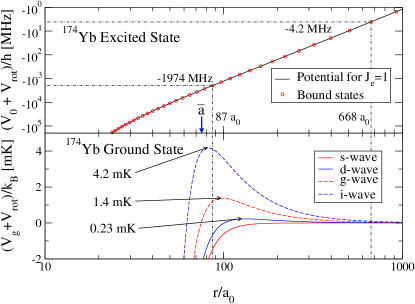
Figure 1: (Color online) The lower and upper panels show $V_{g}+V_{\rm rot}$ and $V_{0}+V_{\rm rot}$, the respective ground state and excited state potentials. The upper curve shows the outer turning points of each calculated $0_{u}^{+}$, $J_{e}=1$ bound level for ¹⁷⁴Yb. The dotted lines indicate the experimentally observed range of levels. The arrow indicates the mean scattering length $\bar{a}=75.18\;a_{0}$. The lower panel shows the centrifugal barriers for the long range ground state potential for $J_{g}=l_{g}=$ 0 ($s$-wave), 2 ($d$-wave), 4 ($g$-wave), and 6 ($i$-wave). An energy $(V_{g}+V_{\rm rot})/k_{B}=$ 1 mK is equivalent to $(V_{g}+V_{\rm rot})/h=$ 21 MHz.

The long-range ground state scattering wave function at very low collision energy depends on three basic parameters, namely the separation between colliding atoms $r$, the relative kinetic energy of collision $\varepsilon_{r}$, and the quantum defect associated with the phase $\Phi$ or, equivalently, the scattering length $a$. The reduced mass $\mu$ is a parameter that allows control of the quantum defect. Thus, the long-range scattering wave function for the van der Waals system has an universal character that can be expressed by a system-independent function of the dimensionless variables $r/\bar{a}$, $\varepsilon_{r}/\bar{\varepsilon}$ and $\mu/\Delta\mu$. All of the needed information about the ground state scattering and bound state wave functions can be calculated from a knowledge of the scaling parameters $r/\bar{a}$, $\varepsilon_{r}/\bar{\varepsilon}$ and $(\mu-\mu_{0})/\Delta\mu$ and the value of reduced mass $\mu_{0}$ for which the scattering length is singular in a given system.

The analytical solutions of the Schrödinger equation are known for several class of potentials, thus allowing the derivations of compact expressions for the scattering length szmytkowski95 . Van der Waals systems such as those discussed here can be nicely described and very well understood using analytical theory. Gao gao00 ; gao01 used the framework of quantum defect theory for a van der Waals system to work out a number of practical formulas and results. For example, when the $s$-wave scattering length is singular, there is a bound state at $E=0$ not only for the $s$-wave but also for $l_{g}=4,8,12,...$. On the other hand if the scattering length is equal to $\bar{a}$ there will be zero energy bound states for $l_{g}=2,6,10,...$. The practical consequence for real potentials is that when the $s$-wave scattering length is near such special values, these other threshold bound states show up as shape resonances for other partial waves. A shape resonance is a quasibound state with enhanced amplitude trapped behind a centrifugal barrier that can lead to enhanced photoassociation. While the wave functions we show are calculated numerically by solving the Schrödinger equation for our potential, the analytic results are very helpful for interpreting their features, and for evaluating approximations like the reflection formula.

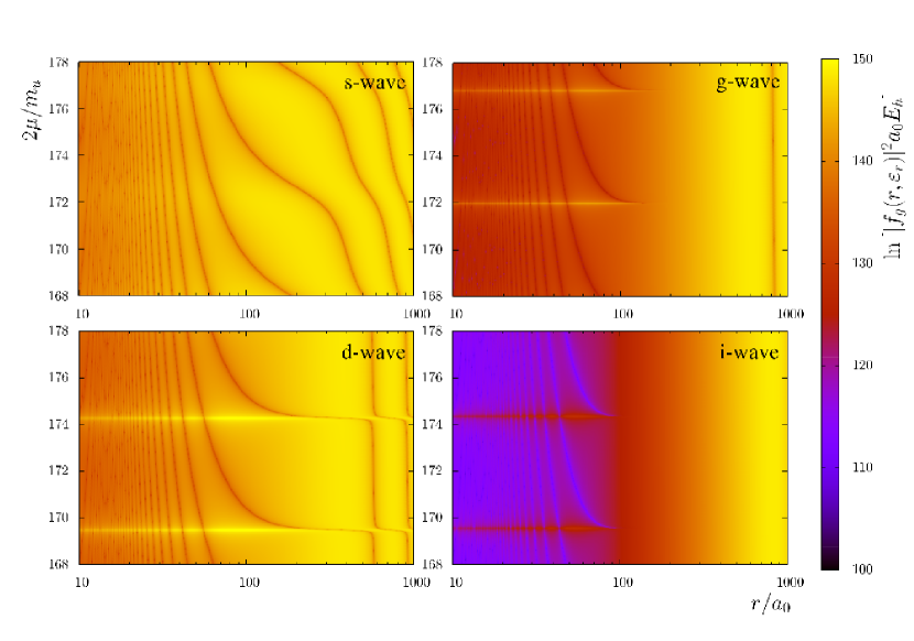
Figure 2: (Color online) The squared magnitude of the numerically calculated scattering wave function $|f_{g}(r,\varepsilon_{r})|^{2}$ of two colliding ground state Yb atoms is shown as a function of intermolecular separation $r$ and reduced mass of colliding system $\mu$, where $m_{u}\approx 1.6605\times 10^{-27}\;{\rm kg}$ . The calculations were carried out for energy of collision $\varepsilon_{r}=100\;\mu K$ and for $J_{g}=l_{g}=$ 0 ($s$-wave), 2 ($d$-wave), 4 ($g$-wave), and 6 ($i$-wave). The dark lines show the nodal lines of the wave functions, whereas the bright areas show the largest amplitudes.

As we already emphasized before, a photoassociation experiment can be used to map the square of the scattering wave function in the ground electronic state at the Condon points corresponding to the different excited bound levels. Figure 1 shows on the lower panel the effective potential, $V_{g}(r)+B(r)J_{g}(J_{g}+1)$, in the ground electronic state, where $J_{g}$ is the rotational quantum number for the partial wave $\ell=J_{g}$. The Fig. 1 shows the centrifugal barrier for a few partial waves with low $J_{g}$. The upper panel of this figure shows the excited state $0_{u}^{+}$ potential together with bound states and their outer turning points, which are essentially the same as their Condon points. This panel shows how the $r_{C}$ value that is probed changes with the binding energy of the excited bound level. Probing experimental levels with binding energies $E_{b}/h$ between 2000 MHz and 3 MHz allow probing the scattering wave function between around 80 a₀ and 800 a₀.

In order to illustrate some properties of the scattering wave function we will begin by setting the collision energy to a constant value corresponding to $\varepsilon_{r}/k_{B}=100$ $\mu$K. As we will show in the next section, shape resonances could be clearly observed at this energy, which is below the top of the $g$-wave centrifugal barrier. Figure 2 shows the dependence of the square of the wave function magnitude on $\mu$ and $r$. Changing $\mu$ corresponds to the change of the quantum defect of the colliding system, which changes $a$ and the bound state spectrum. Calculations have been done for a few lowest partial waves $s$, $d$, $g$, and $i$.

In Fig. 2 the brighter areas show regions of higher amplitude and the dark lines show the nodes of the wave function. The effect of the exclusion of the wave function from short range by the centrifugal barrier is especially evident for the $g$-wave and the $i$-wave. For this Yb system, the singularities in the $s$-wave scattering length occur for $2\mu=$ 167.3, 172.1, and 176.9 $m_{u}$ kitagawa08 . Near these values, an $s$-wave node moves in to smaller distances on the order of $\bar{a}=75.18\;a_{0}$ as $2\mu$ increases and a new bound state appears in the potential. There is also a $g$-wave shape resonance with a dramatic enhancement of short-range amplitude near these $2\mu$ values where $a$ is singular, as expected from the analytic van der Waals quantum defect theory. Similarly, there are $d$- and $i$-wave shape resonances near the values of $2\mu=$ 169.7 and 174.5 $m_{u}$ where $a=\bar{a}$ for the Yb system. Near these shape resonances, a node moves to shorter distances inside the centrifugal barrier as $2\mu$ increases and there is an extra bound state in the potential.

If the collision energy $\varepsilon_{r}$ is lowered, the wave functions show similar patterns, except that the short-range wave function is much more attenuated due to lower penetration through the centrifugal barrier. Clearly, with 28 different physical values for $2\mu$ available, we can expect significant isotopic variation in the photoassociation spectra, depending on the range of Condon points sampled and the temperature of the sample. Spectral lines with Condon points outside of the barrier will have less isotopic sensitivity, whereas lines with Condon points in or inside the region of the barrier will show much more sensitivity to the isotopic combination.

VII Isotopic variation of photoassociation spectra

In this section we will show how the scattering properties of the different Yb isotopes affect their photoassociation spectra. As an example we performed calculations of the light induced trap-loss coefficient at various gas temperatures in range from $10\;{\rm\mu K}$, to $1\;{\rm mK}$. Results for $T=100\;{\rm\mu K}$ are particularly interesting, since the line shapes are relatively sharp and ground scattering resonances can have significant influence on the spectrum. To emphasize the qualitative differences between spectra of the different isotopes we first focus our attention on relatively deep bound states having binding energy around 2000 MHz. As can be seen in Fig. 1 this corresponds to the Condon point placed near or inside the centrifugal barriers.

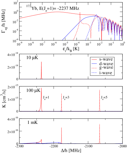
Figure 3: (Color online) Results for the excited $0_{u}^{+}$ bound states of the ¹⁷²Yb₂ molecule near the $J_{e}=1$ level at $E/h=-2237\;$ MHz; other rotational levels with the same vibrational quantum number are evident. The top panel shows contributions to the light induced width $\Gamma_{eg}$ coming from the optical coupling of the ground scattering states having $J_{g}=l_{g}=$ 0 ($s$-wave), 2 ($d$-wave), 4 ($g$-wave), and 6 ($i$-wave) with excited bound states having $J_{e}=J_{g}+1$, as a function of the collision energy $\varepsilon_{r}$, calculated for the light intensity $1\;{\rm W/cm^{2}}$. The $s$-wave scattering length is quite large in magnitude, $-598(63)\;a_{0}$ kitagawa08 , so that this system has a $g$-wave shape resonance near $\varepsilon_{r}/k_{B}=200$ $\mu$K that leads to resonantly enhanced $J_{e}=3$ and 5 features in the photoassociation spectrum. The lower three panels show contributions to the fully thermally averaged loss rate $K$ coming from the optical coupling of the ground scattering states having $J_{g}=l_{g}=$ 0 ($s$-wave), 2 ($d$-wave), 4 ($g$-wave), and 6 ($i$-wave) with excited bound states having $J_{e}=J_{g}+1$ and $J_{e}=J_{g}-1$, as a function of the laser detuning from the atomic resonance, calculated for various temperatures $T=10\;\mu{\rm K}$, $100\;\mu{\rm K}$, and $1\;{\rm mK}$ and the light intensity $0.1\;{\rm mW/cm^{2}}$.

We start our discussion from ¹⁷²Yb which has a large negative scattering length near an $s$-wave singularity kitagawa08 . Consequently, we expect a $g$-wave shape resonance at low scattering energy. The upper panel of Fig. 3 shows the energy dependence of the light induced width for the $J_{e}=$1, 3, 5 and 7 levels with the same vibrational quantum number as the $E(J_{e}=1)/h=-2235\;{\rm MHz}$ level. The light induced widths were calculated for scattering states with total angular momentum $J_{g}=J_{e}-1$. The widths for the same scattering partial wave $J_{g}$ but with $J_{g}=J_{e}+1$ will be very similar in energy variation. The $g$-wave resonance can be clearly seen in upper panel of Fig. 3.

To see how the photoassociation spectrum changes with the temperature of the gas sample we have calculated the thermally averaged light induced trap-loss coefficients for temperatures $T=$10 $\mu$K, 100 $\mu$K and 1 mK; see Fig. 3. These correspond to $kT/h$ of 210 kHz, 2.1 MHz, and 21 MHz respectively. At temperature 10 $\mu$K the spectrum is narrow, with a width determined mainly by the spontaneous emission rate, and is dominated by $s$-wave scattering, for which only the $J_{e}=1$ state is visible. The calculated spectrum at temperature $T=100\;{\rm\mu K}$ has three lines. One is the $J_{e}=1$ line due to $s$-wave scattering. This line has a normal thermal line shape jones06 . Two other strong and sharp lines corresponding to $J_{e}=3$ and $J_{e}=5$ bound states are due to the $g$-wave resonance shown in upper panel of Fig. 3. Both lines have subthermal width; see Ref. machholm02 . The shape of these two lines is determined mostly by the shape of the $g$-wave resonance. Finally, at a temperature of 1 mK one can clearly see the very broad thermally broadened lines coming from $s$ and $d$-wave partial waves. The $d$-wave feature is much broader than the $s$-wave one. This is caused by the fact that for collision energy around 1 mK the light induced width for the $s$-wave decreases with an increase of the collision energy, while for the $d$-wave the light induced width increases. This affects the shape of the line and leads to some shifting and widening of the line coming from the $d$-wave compared to that coming from the $s$-wave. In addition, the $g$-wave shape resonance gives rise to a sharp subthermal feature.

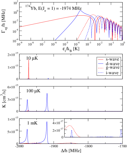
Figure 4: (Color online) Results for the excited $0_{u}^{+}$ bound state of the ¹⁷⁴Yb₂ molecule near the $J_{e}=1$ level at $E/h=-1974$ MHz. The panels are the same as described in the caption of Fig 3. The $s$-wave scattering length is $105(2)\;a_{0}$, which is about $1.4\bar{a}$, and there is a broad $d$-wave shape resonance near $\varepsilon_{r}/k_{B}=220$ $\mu$K near the top of the $d$-wave centrifugal barrier kitagawa08 .

The second example is for ¹⁷⁴Yb, which has a measured scattering length relatively close to $\bar{a}$ kitagawa08 ; enomoto07 . In such case one can expect that both a $d$-wave and an $i$-wave resonance can occur near threshold. As with Fig. 3 for ¹⁷²Yb Fig. 4 shows the light induced width for the ¹⁷⁴Yb bound-states with the total angular momentum $J_{e}=$1, 3, 5 and 7, with the same vibronic quantum number as the level at $E(J_{e}=1)/h=-1973$ MHz. The figure clearly shows the $d$ and $i$-wave resonances. As for ¹⁷²Yb, the spectrum at a temperature of 10 $\mu$K is dominated by the $s$-wave component. However, unlike ¹⁷²Yb, the $d$-wave shape resonance leads to a weak $J_{e}=3$ feature even at such low temperature. The spectra at $T=100$ $\mu$K and 1 mK clearly show the influence of the $d$-wave resonance. This resonance had a crucial role in the correct interpretation of photoassociation spectra near the resonance transition ${}^{1}S_{0}-^{3}P_{1}$ and in the determination of the scattering length for this isotope enomoto07 . When the spectrum is dominated by the features due to the ground state $d$-wave, the intensity ratio of the $J_{e}=3$ and $J_{e}=1$ features should be 3/2 from Eq. (18). Such $d$-wave doublets in ¹⁷⁴Yb were observed by Tojo et al tojo06 , who found that the transition to the bound state with $J_{e}=3$ can be stronger than the transition to $J_{e}=1$ at relatively low collisions energies corresponding to a temperature of about $25\;\mu{\rm K}$, what can be explained by our model.

The spectrum at temperature 1 mK is also dominated by the $d$-wave component. However one can notice sharp structure on the top of a weak and broad feature due to the $J_{e}=5$ bound-state, mostly due to the ground state $g$-wave. The sharp structure is a consequence of the $i$-wave resonance. The $i$-wave component has a subthermal width connected to the $i$-wave resonance seen in upper panel of Fig. 4. One can also notice a weak line corresponding to $J_{e}=7$ bound state supported by this $i$-wave resonance.

Figure 5: (Color online) Results for the excited $0_{u}^{+}$ bound state of the ¹⁷⁶Yb₂ molecule near the $J_{e}=1$ level at $E/h=-1739$ MHz. The panels are the same as described in the caption of Fig 3. The $s$-wave scattering length is $-24(5)\;a_{0}$, not near any special value, but there is a broad $g$-wave shape resonance at relatively high energy near $\varepsilon_{r}/k_{B}=1$ mK near the top of the $g$-wave centrifugal barrier kitagawa08 .

Figure 5 shows our calculations for ¹⁷⁶Yb. This isotope has a relatively small negative scattering length kitagawa08 . The figure shows the light induced width for ¹⁷⁶Yb bound-states with the total angular momentum $J_{e}=$1, 3, 5 and 7, with the same vibronic quantum number as the level at $E(J_{e}=1)/h=-1737\;{\rm MHz}$. Although the scattering length is not near any special value for van der Waals quantum defect theory, a wide $g$-wave resonance is clearly seen relatively high in energy near 1 mK. The spectrum at 10 $\mu$K is typical with only an $s$-wave line that can be observed. Upon increasing the temperature to 100 $\mu$K the spectrum is still dominated by the $s$-wave component, although noticeable $d$-wave components begin to appear. Moreover very weak $g$-wave components occur in this spectrum. The picture changes dramatically when the temperature increases to 1 mK, where the $g$-wave components dominate the spectrum.

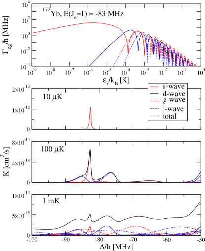
Figure 6: (Color online) Results for the excited $0_{u}^{+}$ bound state of the ¹⁷⁶Yb₂ molecule near the $J_{e}=1$ level at $E=-83$ MHz. The panels are the same as described in the caption of Fig 3. In this case the binding energy is much smaller than in Figs. 3, 4, and 5, and the Condon points are outside the centrifugal barriers except when the collision energy is very low; see Fig. 1.

Finally we would like to show how the spectrum is affected when the Condon point for the transition is moved outside the region of the centrifugal barrier. This is done by choosing a level with much smaller binding energy in our previous examples. Figure 6 shows the light induced width for the ¹⁷²Yb bound-states with the total angular momentum $J_{e}=$1, 3, 5 and 7, with the same vibronic quantum number as the level at $E(J_{e}=1)/h=-83$ MHz. The upper panel of Fig. 6 shows that there are no shape resonances, since there are no amplitude enhancements from being behind the centrifugal barrier. The lower panels of Fig. 6 show the calculated spectra at 10 $\mu$K, 100 $\mu$K, and 1 mK. The higher temperature 100 $\mu$K spectrum is dominated by broad $d$-wave components, on top of which a sharp subthermal $s$-wave component is clearly seen. This is because there is a node in the $s$-wave scattering wave function at the Condon point at relatively low scattering energy, unlike for other partial waves. This sharp structure is a nice example of the subthermal line shapes discussed by Machholm et al. machholm02 in the context of alkaline earth photoassociation. Increasing the temperature to 1 mK leads to a quasi-continuum as several partial waves contribute, as seen from Fig. 6.

The examples in this section show that the photoassociation spectra of various isotopes of the same species can differ qualitatively. This variety is directly connected with the quantum defect in the ground electronic state which is dependent on reduced mass and scattering length of the colliding species. This sensitivity of the rotational structure of photoassociation lines can help in the determination or verification of the scattering length, as it was recently done in case of calcium by Vogt et al. vogt07 .

Figure 7: (Color online) The optical lengths $l^{\rm opt}_{eg}$ of the $s$-wave photoassociation features as a function of the detuning $\Delta$ of the resonance from the atomic transition for the several bosonic isotopes of Yb. The optical length determines the strength of an optical Feshbach resonance. The optical length varies linearly with laser intensity $I$ and these values have been normalized to $I=1\;{\rm W/cm^{2}}$ for $\varepsilon_{r}=0$.

A realistic description of near threshold interaction in the ground and excited electronic states of the Yb₂ molecule is possible thanks to the experimental data tojo06 ; kitagawa08 and the calculations we have shown here. Our models of the interaction potentials can be used to predict the magnitude of the optical lengths in Eq. (6) for the set of optical Feshbach resonances corresponding to the photoassociation lines of the different Yb bosonic isotopes (fermionic isotopes are more complicated because of hyperfine structure in the excited state enomoto08 ). Figure 7 shows our calculated optical lengths for the homonuclear bosonic isotopes of Yb. The isotope ¹⁷²Yb offers the strongest optical Feshbach resonance because of its large negative scattering length, which enhances the amplitude of the $s$-wave ground state wave function in the region of the Condon points. Bound levels near the excited state threshold have optical lengths at 1 W cm^-2 on the order of $10^{6}$ a₀, similar to a value measured for a weakly bound excited level of ⁸⁸Sr zelevinsky06 . This suggests that these resonances may be of practical use for changing the scattering length for useful time scales while reducing spontaneous emission loss processes by using large detuning. Enomoto et al. enomoto08ofr have experimentally demonstrated the possibility of some degree of optical Feshbach control in ultracold Yb gases. Our predicted optical lengths should be helpful in choosing good resonances for controlling ultracold Yb collisions by light.

VIII Conclusion

One could naively think that this is a simple system so that not much difference should be observed between the spectra of three bosonic isotopes like ¹⁷²Yb, ¹⁷⁴Yb, and ¹⁷⁶Yb. However, our calculations show that for temperatures about 100 $\mu$K the spectra for various isotopes are qualitatively different. This difference is manifested by the fact that different rotational lines are apparent in different isotopes. Moreover the shapes of photoassociation lines are also affected. Some lines have subthermal widths depending on the isotope. These differences can be well understood as due to the isotopic variation in the properties of the scattering wave function in the ground electronic state. There is a clear connection between shape resonances in ground scattering states and the appearance of strong lines coming from higher partial waves at relatively low temperature of the order 100 $\mu$K. However, this only happens for excited bound states that have sufficiently short-range Condon points inside the location of the centrifugal barrier. On the other hand, near-threshold bound states with long-range Condon points outside the centrifugal barrier do not show resonance enhancement. For example, we showed that the presence of $J_{e}=3$ lines for ¹⁷²Yb at small detunings does not indicate that a $d$-wave resonance occurs. Thus, a good experimental method to determine whether resonances are present or not would be to measure photoassociation lines for more deeply bound excited states that have turning points near to or less that the ground state centrifugal barrier. The existence of resonances correlates with the approximate value of the $s$-wave scattering length.

The intercombination photoassociation spectra of Yb are qualitatively different from spectra for group II atoms such as Ca and Sr. For the case of Ca theory shows that the excited state potential in the turning point range for levels near the dissociation limit is dominated by the van der Waals potential, since the resonant dipolar interaction is so small ciurylo04 ; bussery05 . The reflection approximation is not applicable in such a case ciurylo06 . Strontium zelevinsky06 is a system which is half way between Ca and Yb. Only the last three Sr bound states closest to the dissociation limit can be treated as dominated by the resonant dipole interaction, while more deeply bound levels are determined mostly by the van der Waals part of the interaction. Photoassociation can be observed in Ca or Sr for two series of bound states of $0_{u}^{+}$ and $1_{u}$ symmetry, respectively. Although the resonant dipole interaction for the $1_{u}$ state is repulsive, its weakness allows it to be overcome by the attractive van der Waals interaction. In contrast the Yb interaction in the excited electronic state with dissociation limit ${}^{1}S_{0}+^{3}P_{1}$ is dominated by the resonance interaction, so that only one potential curve of $0_{u}^{+}$ symmetry is attractive at long range and supports a series of detectable bound states. The reflection approximation is well applicable in the case of $0_{u}^{+}$ levels of Yb. Since the $1_{u}$ potential becomes attractive at much shorter range of the interatomic separation, the density of bound states near threshold is much less, and only one bound state with $1_{u}$ symmetry is expected near within a few GHz of threshold.

The heavier group IIb elements such as Cd and Hg will be similar to Yb. For both species the interaction in the excited state is dominated by the resonance interaction, and therefore one can expect that the reflection approximation will be applicable. Moreover both species have numerous stable isotopes. Consequently, mass tuning of the scattering length should be applicable for both of these species, and the results obtained in this work can be treated as universal and generic for Cd and Hg.

- (1) T. Ido, H. Katori, Phys. Rev. Lett. 91, 053001 (2003).
- (2) E. A. Curtis, C. W. Oates, and L. Hollberg, J. Opt. Soc. Am. B 20, 977 (2003).
- (3) T. H. Loftus, T. Ido, M. M. Boyd, A. D. Ludlow, and J. Ye, Phys. Rev. A 70, 063413 (2004).
- (4) G.Wilpers, T. Binnewies, C. Degenhardt, U. Sterr, J. Helmcke, and F. Riehle, Phys. Rev. Lett. 89, 230801 (2002).
- (5) Z. W. Barber, C. W. Hoyt, C. W. Oates, L. Hollberg, A. V. Taichenachev, and V. I. Yudin, Phys. Rev. Lett. 96, 083002 (2006).
- (6) R. Le Targat, X. Baillard, M. Fouché, A. Brusch, O. Tcherbakoff, G. D. Rovera, and P. Lemonde, Phys. Rev. Lett. 97, 130801 (2006).
- (7) M. M. Boyd, A. D. Ludlow, S. Blatt, S. M. Foreman, T. Ido, T. Zelevinsky, and J. Ye, Phys. Rev. Lett. 98, 083002 (2007).
- (8) Y. Takasu, K. Maki, K. Komori, T. Takano, K. Honda, M. Kumakura, T. Yabuzaki, and Y. Takahashi, Phys. Rev. Lett. 91, 040404 (2003).
- (9) T. Fukuhara, S. Sugawa, and Y. Takahashi, Phys. Rev. A 76, 051604(R) (2007).
- (10) T. Fukuhara, S. Sugawa, Y. Takasu, and Y. Takahashi, Phys. Rev. A 79, 021601(R) (2009).
- (11) T. Fukuhara, Y. Takasu, M. Kumakura, and Y. Takahashi, Phys. Rev. Lett. 98, 030401 (2007).
- (12) Y. Takasu, K. Komori, K. Honda, M. Kumakura, T. Yabuzaki, and Y. Takahashi, Phys. Rev. Lett. 93 123202 (2004).
- (13) S. Tojo, M. Kitagawa, K. Enomoto, Y. Kato, Y. Takasu, M. Kumakura, and Y. Takahashi, Phys. Rev. Lett. 96, 153201 (2006).
- (14) K. Enomoto, M. Kitagawa, S. Tojo, and Y. Takahashi, Phys. Rev. Lett. 100, 123001 (2008).
- (15) M. Kitagawa, K. Enomoto, K. Kasa, Y. Takahashi, R. Ciuryło, P. Naidon, and P. S. Julienne, Phys. Rev. A 77, 012719 (2008).
- (16) K. Enomoto, K. Kasa, M. Kitagawa, Y. Takahashi, Phys. Rev. Lett. 101, 203201 (2008).
- (17) K.-A. Brickman, M.-S. Chang, M. Acton, A. Chew, D. Matsukevich, P. C. Haljan, V. S. Bagnato, and C. Monroe, Phys. Rev. A 76, 043411 (2007).
- (18) T. Walther, J. Mod. Opt. 54, 2523 (2007).
- (19) H. Hachisu, K. Miyagishi, S. G. Porsev, A. Derevianko, V. D. Ovsiannikov, V. G. Pal’chikov, M. Takamoto, and H. Katori Phys. Rev. Lett. 100, 053001 (2008).
- (20) S. G. Porsev, A. Derevianko, Phys. Rev. A 74, 020502R (2006).
- (21) J. Weiner, V. S. Baganato, S. Zilio, and P. S. Julienne, Rev. Mod. Phys. 71, 1 (1999).
- (22) R. Ciuryło, E. Tiesinga, S. Kotochigova, and P. S. Julienne, Phys. Rev. A 70, 062710 (2004).
- (23) R. Napolitano, J. Weiner, C. J. Williams, and P. S. Julienne, Phys. Rev. Lett. 73, 1352 (1994).
- (24) P. S. Julienne, J. Res. Natl. Inst. Stand. Technol. 101, 487 (1996).
- (25) J. L. Bohn and P. S. Julienne, Phys. Rev. A 60, 414 (1999).
- (26) R. Napolitano, J. Weiner, and P. S. Julienne, Phys. Rev. A 55, 1191 (1997).
- (27) U. Fano, Phys. Rev. 124, 1866 (1961).
- (28) A. Simoni, P. S. Julienne, E. Tiesinga, and C. J. Williams, Phys. Rev. A 66, 063406 (2002).
- (29) P. O. Fedichev, Yu. Kagan, G. V. Shlyapnikov, and J. T. M. Walraven, Phys. Rev. Lett. 77, 2913 (1996).
- (30) J. L. Bohn and P. S. Julienne, Phys. Rev. A 56, 1486 (1997).
- (31) F. K. Fatemi, K. M. Jones, and P. D. Lett, Phys. Rev. Lett. 85, 4462 (2000).
- (32) M. Theis, G. Thalhammer, K. Winkler, M. Hellwig, G. Ruff, R. Grimm, and J. Hecker Denschlag, Phys. Rev. Lett. 93, 123001 (2004).
- (33) G. Thalhammer, M. Theis, K. Winkler, R. Grimm, and J. Hecker Denschlag, Phys. Rev. A 71, 033403 (2005).
- (34) R. Ciuryło, E. Tiesinga, and P. S. Julienne, Phys. Rev. A 71, 030701R (2005).
- (35) C. Chin, R. Grimm, P. S. Julienne, and E. Tiesinga, e-print arXiv:0812.1486.
- (36) P. S. Julienne and F. H. Mies, Phys. Rev. A 34, 3792 (1986).
- (37) T. Zelevinsky, M. M. Boyd, A. D. Ludlow, T. Ido, J. Ye, R. Ciuryło, P. Naidon, and P. S. Julienne, Phys. Rev. Lett. 96, 203201 (2006).
- (38) M. Machholm, P. S. Julienne, and K.-A. Suominen, Phys. Rev. A 64, 033425 (2001).
- (39) F. Vogt, Ch. Grain, T. Nazarova, U. Sterr, F. Riehle, Ch. Lisdat, and E. Tiemann, Eur. Phys. J. D 44, 73 (2007).
- (40) C. Boisseau, E. Audouard, J. Vigue, and P. S. Julienne, Phys. Rev. A 62, 052705 (2000).
- (41) R. Ciuryło, E. Tiesinga, and P. S. Julienne, Phys. Rev. A 74, 022710 (2006).
- (42) K. M. Jones, E. Tiesinga, P. D. Lett, and P. S. Julienne, Rev. Mod. Phys. 78, 483 (2006)
- (43) E. G. M. van Kempen, S. J. J. M. F. Kokkelmans, D. J. Heinzen, and B. J. Verhaar, Phys. Rev. Lett. 88, 093201 (2002).
- (44) Y. Wang and M. Dolg, Theor. Chem. Acc. 100, 124 (1998).
- (45) E. A. Power, J. Chem. Phys. 46, 4297 (1967).
- (46) W. J. Meath, J. Chem. Phys. 48, 227 (1968).
- (47) P. Zhang and A. Dalgarno, Mol. Phys. 106, 1525 (2008); J. Phys. Chem. A 111, 12471 (2007).
- (48) A. A. Buchachenko, G. Chałasiński, and M. M. Szczśniak, Eur. Phys. J. D 45, 147 (2007).
- (49) Y. N. Martinez de Escobar, P. G. Mickelson, P. Pellegrini, S. B. Nagel, A. Traverso, M. Yan, R. Côté, and T. C. Killian, Phys. Rev. A 78, 062708 (2008).
- (50) A. Stein, H. Knöckel, and E. Tiemann, Phys. Rev. A 78, 042508 (2008).
- (51) G. F. Gribakin and V. V. Flambaum, Phys. Rev. A 48, 546 (1993).
- (52) V. V. Flambaum, G. F. Gribakin, and C. Harabati, Phys. Rev. A 59, 1998 (1999).
- (53) C. Boisseau, E. Audouard, J. Vigue, and V. V. Flambaum, Eur. Phys. J. D 12, 199 (2000).
- (54) R. Szmytkowski, J. Phys. A 28, 7333 (1995).
- (55) B. Gao, Phys. Rev. A 62, 050702(R) (2000).
- (56) B. Gao, Phys. Rev. A 64, 010701(R) (2001).
- (57) M. Machholm, P. S. Julienne, and K. A. Suominen, Phys. Rev. A 65, 023401 (2002).
- (58) K. Enomoto, M. Kitagawa, K. Kasa, S. Tojo, and Y. Takahashi, Phys. Rev. Lett. 98, 203201 (2007).
- (59) B. Bussery-Honvault, J.-M. Launay, and R. Moszyński, Phys. Rev. A 72, 012702 (2005).