Extreme value statistics and return intervals in long-range correlated uniform deviates

Abstract

We study extremal statistics and return intervals in stationary long-range correlated sequences for which the underlying probability density function is bounded and uniform. The extremal statistics we consider (e.g. maximum relative to minimum) are such that the reference point from which the maximum is measured is itself a random quantity. We analytically calculate the limiting distributions for independent and identically distributed random variables, and use these as a reference point for correlated cases. The distributions are different from that of the maximum itself (i.e. a Weibull distribution), reflecting the fact that the distribution of the reference point either dominates over or convolves with the distribution of the maximum. The functional form of the limiting distributions is unaffected by correlations, although the convergence is slower. We show that our findings can be directly generalized to a wide class of stochastic processes. We also analyze return interval distributions, and compare them to recent conjectures of their functional form.

I Introduction

Interest in the extreme behavior of complex systems has been growing, with examples including the estimation of DNA replication times Bechhoefer and Marshall (2007), extreme paths on random trees Majumdar and Krapivsky (2000); Ben-Naim et al. (2001) and their applications to computer science Majumdar and Krapivsky (2002), extreme eigenvalues in random matrices and low-lying states in disordered systems Bouchaud and Mézard (1997); Biroli et al. (2007), and extreme values in multifractal processes Muzy et al. (2006). In particular, much attention has been paid to extreme value statistics in time series. This is especially relevant in the context of disasters and hazard assessment Bunde et al. (2002), flood prediction being a notable example Battjes and Gerritsen (2002). In regard to this, results exist in the mathematical literature Leadbetter et al. (1983) which extend the range of extreme limit distributions based on identically and independently distributed (iid) random variables to a wide class of dependent time series, see Leadbetter and Rootzén (1988) for a review. Yet, the exact extremal properties of many time series exhibiting long-range correlations are far from being fully understood. Examples of such time series in nature include crackling noise Sethna et al. (2001), water levels in rivers Hurst (1951), temperature fluctuations in oceans Monetti et al. (2003), or climatological temperature records Pelletier and Turcotte (1997); Huybers and Curry (2006). Much insight into the extremes of these time series can be gained by studying so-called $1/f^{\alpha}$ signals Majumdar and Comtet (2004); Györgyi et al. (2007); Burkhardt et al. (2007) (in reference to the power-law decay of the power spectrum), which capture many of the essential features of real-world long-range correlated time series.

Aside from the distribution of extremes, another very useful and practical indicator for hazard assessment based on time series is the distribution of return intervals between successive threshold-crossing events. For uncorrelated time series, the Poisson process gives rise to the well-known exponential return interval distribution Cox and Isham (1980). For long-range correlated series encountered in nature, however, the distribution is no longer exponential and a number of distributions have been put forward, depending on the data set, such as gamma distributions and power-laws with stretched exponential tails Corral (2004); Davidsen et al. (2007); Baiesi et al. (2006); Bunde et al. (2005); Vázquez et al. (2006). Artificially generated $1/f^{\alpha}$ signals have been studied in detail Altmann and Kantz (2005); Eichner et al. (2007) and some progress has been made towards a theoretical understanding of return intervals in long-range correlated series Corral (2005); Sornette et al. (2008); Santhanam and Kantz (2008), but the overall picture is far from complete.

Here, we focus on the extremal properties and return intervals of stationary long-range correlated series for which the underlying probability density function (PDF) is uniform over a given finite interval, i.e. the $X_{i}$ that make up the series $\{X_{i}\}_{i=1\dots n}$ are uniformly distributed. These processes are of general interest and have been neglected in the past. For iid random variables, a single parameter family of distributions describes the possible limiting distribution for the maximum of a sample de Haan and Ferreira (2006). This family is traditionally broken up into three qualitatively different distributions: Fréchet, Gumbel and Weibull. Provided certain conditions are met, a given underlying PDF for the iid random variables will fall within the domain of attraction of one of these three extreme value distributions. Previous studies have concentrated on time series with underlying PDF that belong to the Gumbel or Fréchet domains of attraction. Random variables distributed uniformly on $[0,1]$, however, belong to the Weibull domain of attraction . In fact, the same is true for a series of stationary long-range correlated uniform deviates, provided certain mixing criteria are met Leadbetter et al. (1983); Leadbetter and Rootzén (1988). However, we show in this paper that a variety of extremal quantities converge to very different limiting distributions. When the maximum is measured relative to a quantity that is itself a random variable, the extremal distribution need no longer be Gumbel, Fréchet or Weibull. In this paper we consider the following three extremal quantities: (a) maximum relative to the average (over the $X_{i}$), introduced in the context of interfaces Raychaudhuri et al. (2001), (b) maximum relative to the initial value Burkhardt et al. (2007); Sabhapandit and Majumdar (2007), which is a natural measure in the context of time series (e.g. the maximum increase of a stock from its starting price), (c) maximum relative to minimum, which is a measure of the full range of values encountered (e.g. as measured in auroral indices Hnat et al. (2002)).

The structure of the paper is as follows: In Section II we present analytic results for extremal distributions for iid random variables and we briefly discuss how our results may be generalised to other distributions belonging to the Weibull class, e.g. the beta distribution. In Section III, we then compare the iid results to the respective distributions in stationary long-range correlated series. In Section IV we present the corresponding return interval distributions and examine their asymptotic behavior. We conclude the paper in Section V. In an Appendix, we discuss some of the features of the Schreiber-Schmitz algorithm Schreiber and Schmitz (1996, 2000) for generating long-range correlated series with a specified underlying PDF.

II Extremal statistics for iid uniform deviates

Consider a set of $n$ iid random variables $\{X_{1},\ldots,X_{n}\}$ drawn from the (cumulative) distribution function $F(z)$. The distribution of the maximum $M_{n}$ is

$$\text{Pr}(M_{n}\leq z) =\text{Pr}(X_{1}\leq z,\ldots,X_{n}\leq z)$$

$$=F^{n}(z)$$ (1)

A fundamental result of extreme value theory is that if $F^{n}(a_{n}z+b_{n})$ converges to a non-degenerate limiting distribution as $n\to\infty$, where $a_{n}$ and $b_{n}$ are scale and location parameters, respectively, that effect a linear rescaling, the distribution can be one of only three types. The eventual limiting distribution is determined by the asymptotic behavior of the underlying $F(z)$ de Haan and Ferreira (2006). For the specific example of $n$ iid uniform deviates with probability density $p(z)=1$ for $0\leq z\leq 1$, the choice $a_{n}=1/n,b_{n}=1$ gives

$$\lim_{n\to\infty}F^{n}(z/n+1) =\lim_{n\to\infty}(z/n+1)^{n}$$

$$=e^{z},$$ (2)

which is an example of a Weibull distribution. While the choice of $a_{n}$ and $b_{n}$ is not unique, the particular choice does not influence the functional form of the limiting distribution according to the Khinchin theorem Leadbetter et al. (1983). It does, however, determine convergence rates Györgyi et al. (2008). In this paper we choose $a_{n}$ and $b_{n}$ so that all limiting PDFs $p(y)=\frac{dF(y)}{dy}$ are standardized with zero mean (via the location parameter) and unit standard deviation (via the scale parameter), where $y:=a_{n}z+b_{n}$. That is,

$$\int z\,dF^{n}(a_{n}z+b_{n}) =0$$ (3)

$$\int z^{2}\,dF^{n}(a_{n}z+b_{n}) =1.$$ (4)

II.1 Maximum relative to average

Labelling the maximum as $x^{max}_{n}$, the maximum relative to the average is defined as $z:=x_{n}^{max}-\frac{1}{n}\sum_{i=1}^{n}x_{i}$. By the central limit theorem, the average of $n$ iid uniform deviates approaches a Gaussian distribution centered at $1/2$ with a width that shrinks as $\mathcal{O}(n^{-1/2})$. The choice of $a_{n}=1/n$ in Eq. (2) shows that the maximum approaches $1$ as an exponential distribution with a width that shrinks as $\mathcal{O}(n^{-1})$. The scaling of $a_{n}$ is, to leading order, generic up to prefactors Leadbetter et al. (1983). Therefore, as $n\to\infty$, the spread in the average dominates, and the PDF of the maximum relative to the average is

$$p(y)=\frac{1}{\sqrt{2\pi}}e^{-y^{2}/2},$$ (5)

with zero mean and unit standard deviation.

II.2 Maximum relative to initial value

Given an initial value $x_{1}$, the maximum relative to the initial value is defined as $z:=x^{max}_{n}-x_{1}$. The initial value is a random variable with a distribution having a width of $\mathcal{O}(1)$. Therefore, by the same argument as above, only the spread in the initial value is observed for $n\to\infty$. Specifically, two situations must be distinguished. With probability $1/n$, the initial value is itself the maximum, yielding a zero maximum relative to the initial value. Thus the distribution is composed of a point mass of weight $1/n$ at $z=0$. For $z>0$, the probability distribution is continuous and the calculation of the probability density is as follows: without loss of generality, label from among the remaining $(n-1)$ random variables the maximum as the final one. Then

$$p(z) =(n-1)\int_{0}^{x_{n}}dx_{1}\cdots\int_{0}^{x_{n}}dx_{n-1}\int_{0}^{1}dx_{n}$$

$$\times\prod_{i=1}^{n}\theta(x_{i})\theta(1-x_{i})\delta(z-(x_{n}-x_{1}))$$

$$=1-z^{n-1},$$ (6)

where $(n-1)$ is a combinatorial factor taking into account all possible locations of the maximum among the remaining $(n-1)$ random variables.

Substituting the PDF in Eq. (6) into Eqs. (3),(4), the location and scale parameters that maintain zero mean and unit standard deviation are

$$b_{n} =\frac{1}{2}\frac{n}{(n+1)}=\frac{1}{2}-\frac{1}{2n}+\mathcal{O}(n^{-2})$$ (7)

$$a_{n} =\frac{\sqrt{3}}{6}-\frac{1}{4}\frac{\sqrt{3}}{n}+\mathcal{O}(n^{-2}).$$ (8)

Thus, to leading order, the location and scale parameters are simply the mean and standard deviation of the uniform distribution. As $n\to\infty$ the rescaled PDF of the maximum relative to the initial value converges to

$$p(y)=\begin{cases}\sqrt{3}/6,&\quad-3/\sqrt{3}\leq y\leq 3/\sqrt{3}\\ 0,&\quad\text{otherwise.}\end{cases}$$ (9)

For more general cases, see Burkhardt et al. (2007).

II.3 Maximum relative to minimum

Without loss of generality, labelling the minimum and the maximum as the first and last random variables, respectively, the distribution of the maximum relative to the minimum, $z:=x_{n}-x_{1}$ is given by

$$p(z) =n(n-1)\int_{0}^{x_{n}}dx_{1}\int_{x_{1}}^{x_{n}}dx_{2}\cdots\int_{x_{1}}^{x_{n}}dx_{n-1}\int_{0}^{1}dx_{n}$$

$$\times\prod_{i}^{n}\theta(x_{i})\theta(1-x_{i})\delta(z-(x_{n}-x_{1}))$$

$$=n(n-1)z^{(n-2)}(1-z),$$ (10)

where $n(n-1)$ is a combinatorial factor taking into account all possible locations of the maximum and the minimum among the $n$ variables.

Substituting the PDF in Eq. (10) into Eqs. (3),(4) the location and scale parameters that maintain zero mean and unit standard deviation are

$$b_{n} =\frac{n-1}{n+1}=1-\frac{2}{n}+\mathcal{O}(n^{-2})$$ (11)

$$a_{n} =\frac{\sqrt{2}}{n}+\mathcal{O}(n^{-2}).$$ (12)

To leading order, the location parameter reflects the fact that the distribution centers at $z=1$ from below as $n\to\infty$. Meanwhile, the scale parameter reflects the fact that the width of the distribution shrinks as $\mathcal{O}(n^{-1})$ to leading order. As $n\to\infty$ the rescaled PDF of the maximum relative to the initial value converges to

$$p(y)=\sqrt{2}(2-\sqrt{2}y)e^{\sqrt{2}y-2},\quad-\infty<y\leq\sqrt{2},$$ (13)

and zero otherwise.

II.4 Other distributions belonging to the Weibull class

While the results given in Sections II.1–II.3 are for the uniform distribution, the arguments used in their derivation can be easily generalized to any other distribution. Namely, the widths under rescaling of the maximum and the reference value should be compared in order to determine the final limiting distribution for the extremal statistic. Generally, either one or the other will dominate, apart from the special case when both widths are rescaled in the same way, in which case there will be a convolution of the two distributions (assuming that the $n$-independent prefactors are comparable in magnitude). This is in particular true for another prominent example in the Weibull class, the beta distribution, with PDF

$$p(z)=\frac{z^{\gamma-1}(1-z)^{\delta-1}}{B(\gamma,\delta)},\quad 0\leq z\leq 1,$$ (14)

and zero otherwise, where $\gamma,\delta>0$ and $B(\gamma,\delta)$ is the beta function. The maxima of the beta distribution are Weibull-distributed, provided the width is rescaled with $a_{n}\sim n^{-1/\delta}$. Thus, for example, the maximum measured with respect to the average yields a Gaussian, a convolution, and a Weibull distribution for $\delta<2$, $\delta=2$ and $\delta>2$, respectively.

III Extremal statistics for stationary long-range correlated signals

The stationary long-range correlated series $X_{i}$ of length $n$ that we study have a uniform underlying PDF on $[0,1]$ and two-time correlation function that decays as

$$C_{ij}=\langle X_{i}X_{j}\rangle-\langle X_{i}\rangle\langle X_{j}\rangle\sim|i-j|^{-(1-\alpha)},$$ (15)

where the average corresponds to an ensemble average. Stationarity requires that $\alpha<1$ and long-range correlations are those for which $0<\alpha<1$. By the Wiener-Khinchin theorem, the Fourier transform of the two-time correlation function is simply the power spectrum and both are equivalent descriptions. For stationary long-range correlated series, it follows that the power spectrum decays as $1/f^{\alpha}$.

In order to generate series of long-range correlated uniform deviates, we employ the algorithm of Schreiber and Schmitz Schreiber and Schmitz (1996, 2000). The method works iteratively to enforce a desired power spectrum by permuting iid random variables drawn from a desired distribution. Each iteration consists of two steps: adjusting the power spectrum of the random variables in Fourier space with the appropriate filter, and then rank-order exchanging the reversed-transformed variables with the original iid random variables. Thus, the algorithm does not change the values of the variables drawn initially, but does change their order. For the uniform distribution, only a small number of iterations is required for the power spectrum to converge to the desired form – in our case, a power-law with slope $-\alpha$. More details of the method are outlined in the Appendix.

The statistics for the extremal quantities are collected in segments. Typically, we generated series of length $2^{19}$ to $2^{22}$, cut up $2^{7}$ to $2^{10}$ times to produce blocks of length $2^{11}$ to $2^{15}$. The process is repeated for a number of generated series to produce histograms with $\mathcal{O}(10^{6}-10^{7})$ points. The histograms are normalized and rescaled to give $p(y)$, with zero mean and unit standard deviation.

As mentioned in the introduction, the three classes of extreme distributions for the maxima of iid random variables remain robust for a wide class of dependent series Leadbetter et al. (1983), including, for example, long-range correlated Gaussian series Berman (1964). Numerically, we find that this is also true for the long-range correlated uniform processes defined above. This suggests that the relevant mixing conditions are satisfied for the case of long-range correlated uniform deviates, although we have not checked this analytically . Moreover, while there are strong finite size corrections to the variation of the scale parameter $a_{n}$ with $n$, even the asymptotic behavior or leading order scaling is identical to the iid case, $a_{n}=1/n$. Our numerics indicate that for small system sizes the higher order corrections are positive. Such a behavior is not generally expected since, owing to correlations, the leading order scaling of $a_{n}$ may be different than those in the iid case Leadbetter et al. (1983). In the following, we show that analogous results hold for the three relative maxima, i.e., the distributions derived in Eqs. (5),(9),(13) for iid random variables also apply to the dependent case.

III.1 Maximum relative to average

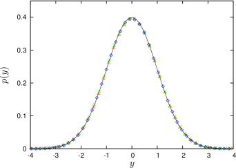
Fig. 1 plots the maximum relative to the average for blocks of length $2^{11},2^{13},2^{15}$ (triangles, crosses, diamonds) and $\alpha=0.5$. The curves are barely distinguishable from the iid limiting Gaussian distribution, and the convergence is rapid for the system sizes examined. Numerically, we find that the same holds for $0\leq\alpha<1$ (not shown). These results are expected since the width of the limiting Gaussian distribution of the average decays as $n^{(\alpha-1)/2}$ Bouchaud and Georges (1990); Ibragimov and Linnik (1971) while the width of the distribution of the maximum decays asymptotically as $n^{-1}$ as mentioned above. Thus, the average dominates for any $\alpha$ implying that a Gaussian distribution is observed asymptotically.

Figure 1: (Color online) Distribution of maximum relative to average for sequences of length $2^{11},2^{13},2^{15}$ (triangles, crosses, diamonds) and $\alpha=0.5$, with zero mean and unit standard deviation. A Gaussian is plotted alongside as a solid line.

III.2 Maximum relative to initial value

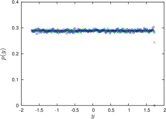
Fig. 2 plots the maximum relative to the initial value for blocks of length $2^{11},2^{13},2^{15}$ (triangles, crosses, diamonds) and $\alpha=0.5$. The curves closely follow a straight horizontal line of height $\sqrt{3}/6$. We find the same behavior for other $\alpha$ with $0\leq\alpha<1$ (not shown). If we assume that the distribution approaches the same limit as in the iid case, then the exact form for finite $n$ is given by Eq. (6). The function approaches zero at its upper endpoint very rapidly, and this feature is also observed in Fig. 2 for the dependent case.

Figure 2: (Color online) Distribution of maximum relative to initial value for sequences of length $2^{11},2^{13},2^{15}$ (triangles, crosses, diamonds) and $\alpha=0.5$, with zero mean and unit standard deviation. A uniform distribution is plotted alongside as a solid line.

Since the distribution consists of a point mass at zero maximum relative to the initial value, it is particularly convenient to analyze this behavior with increasing $\alpha$. Fig. 3 demonstrates that the fraction $p$ of times when the initial value is also the maximum decreases as $1/n$.

Figure 3: (Color online) Decay in the fraction of zero maxima relative to initial value with increasing system size, for $\alpha=0.95,0.8,0.6,0.4,0.2$ (top to bottom). The decay $1/n$ for iid series is shown by the solid black line.

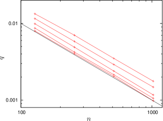
However, the amplitude of the decay increases with $\alpha$. An intuitive explanation for this behavior is as follows: persistence along the series increases with $\alpha$, i.e. the series has memory and is more likely to continue in the same direction as previously. A series that starts with a downward trend is more likely to produce a zero maximum relative to the initial value. Such persistent trajectories are more prevalent with increasing $\alpha$, and therefore the amplitude of the point mass is enhanced relative to the iid case.

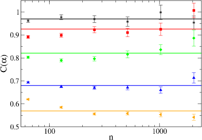
In the presence of correlations, convergence to limiting distributions is typically slower than in the iid case Coles (2001). The effect of increasing $\alpha$ (i.e. correlations) can be taken into account by replacing the block size $n$ by a smaller size $n_{\text{eff}}=C(\alpha)n$, where $C(\alpha)<1$ is an $\alpha$-dependent constant. If we assume a similar behavior for the maximum measured relative to the minimum, then the simplest modification to Eq. (6) for correlated series would consist of a point mass with weight $1/(C(\alpha)n)$ at zero, together with a density

$$p(z)=1-z^{C(\alpha)n-1}$$ (16)

for $z>0$. Fig. 4 plots estimates of $C(\alpha)$ for various $\alpha$, suggesting that a decreased effective degrees of freedom description is valid.

Figure 4: (Color online) Measurements of $C(\alpha)$ based on Eq. (16) for $\alpha=0.2,0.4,0.6,0.8,0.95$ (top to bottom) and $n=64,128,256,512,1024,2048$. For each $\alpha$, the lines are averages over the six system sizes. Error bars are estimates of statistical error (via standard error propagation) and represent one standard deviation: over $N$ measurements the number of instances of the maximum also being the initial value is binomially distributed with expectation $Np$ and variance $Np(1-p)$, where $p=1/n$ is the probability that the maximum lies at the initial value.

III.3 Maximum relative to minimum

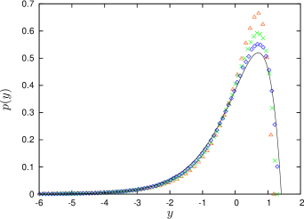
Fig. 5 plots the maximum relative to the minimum for blocks of length $2^{11},2^{13},2^{15}$ (red, green, blue) and $\alpha=0.5$. Convergence is evidently slower for this maximal quantity and worsens with increasing $\alpha$ (not shown). We speculate that this is because the maximum and minimum approach their respective limiting distributions at the same rate, giving rise to the convoluted distribution derived in Eq. (10) in the iid case.

Figure 5: (Color online) Distribution of maximum relative to minimum for sequences of length $2^{11},2^{13},2^{15}$ (triangles, crosses, diamonds) and $\alpha=0.5$, with zero mean and unit standard deviation. The distribution in Eq. (13) is plotted alongside as a solid line.

III.4 Other distributions belonging to the Weibull class

For long-range correlated processes obeying the beta distribution defined in Eq. (14), the same picture emerges as above once the relative rescalings of the maximum and the respective reference value are taken into account. Our numerics num indicate that the distribution of the maxima and the minima both approach a Weibull distribution and that $a_{n}$ scales asymptotically as $n^{-1/\delta}$ for the maximum and $n^{-1/\gamma}$ for the minimum — as in the iid case. As in the case of the uniform distribution, the width of the limiting Gaussian distribution of the average scales as $n^{(\alpha-1)/2}$. Thus, depending on the particular choice of $\alpha$, $\gamma$ and $\delta$, different limiting distributions are obtained. For example, for $\gamma=\delta=2$ the extremal statistics obey respectively a Gaussian, a beta distribution with $\gamma=\delta=2$, and a convoluted distribution for the maximum measured with respect to the average, initial value, and minimum.

In general, if a given Weibull process satisfies the relevant mixing conditions Leadbetter et al. (1983) and $a_{n}$ scales asymptotically like its uncorrelated counterpart, then, barring slow convergence, one of three scenarios will occur: (a) the width of the maximum distribution shrinks slower than that of the reference, in which case the maximum distribution is observed, (b) the width of the reference distribution shrinks slower than that of the maximum, in which case the reference distribution is observed, (c) the widths of the maximum and reference distributions scale at the same rate and are of comparable amplitude, in which case a non-trivial convolution is observed.

IV Return times

Return times are useful indicators for analyzing time series and are particularly relevant when forecasting extreme events, e.g. floods or large earthquakes. For example, a flood levee may be constructed so as to permit flooding only once every $10,000$ years, on average. Supposing that at time $t_{i}$ an event of magnitude $x_{i}$ exceeds some threshold $q$, and that the threshold is subsequently exceeded for the first time by an event $x_{j}$ at $t_{j}$, then the return time is defined as $t:=t_{j}-t_{i}$. Since in our context time marches in unit steps, the smallest return time is $1$, i.e. as a result of two consecutive events that exceed the threshold.

In our simulations we generate series of length $2^{19},\ldots,2^{22}$ a repeated number of times ($\sim 10^{2}$ to $10^{5}$). The return times derived from these series are then combined into a histogram, from which we construct the normalized return time distribution $p(t)$.

The iid scenario is described by a Poisson point process, giving exponentially distributed return times. For stationary long-range correlated series, meanwhile, the authors of Eichner et al. (2007); Altmann and Kantz (2005) proposed the following fit-free (but nevertheless $\alpha$-dependent) ansatz for the return time distribution:

$$\tau p(t)=a_{\alpha}\exp{[-b_{\alpha}(t/\tau)^{1-\alpha}]},$$ (17)

where $\tau$ is the mean return time, and $a_{\alpha}$ and $b_{\alpha}$ are $\alpha$-dependent constants of normalization fixed by

$$\sum_{t=1}^{\infty}p(t) =1,$$ (18)

$$\sum_{t=1}^{\infty}tp(t) =\tau.$$ (19)

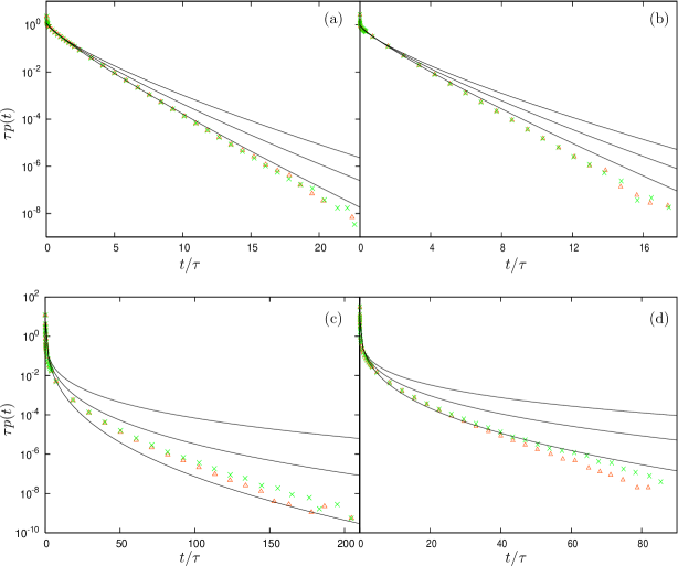
We test this stretched exponential ansatz for long-range correlated uniform deviates. Fig. 6(a),(b) plots numerical results for $\alpha=0.2$ and two different quantiles. Stretched exponential curves are drawn alongside for $\alpha=0.25,0.2,0.15$ from top to bottom. In Fig. 6(a) the errors are within the symbol size up to $t/\tau\approx 16$, with larger statistical fluctuations thereafter. For Fig. 6(b), errors remain within symbol size up to $t/\tau\approx 13$. The agreement between the numerical results and the ansatz is poor. Increasing the quantile worsens the agreement. For the results shown, there appears to be no systematic trend towards the ansatz with increasing system size. Figs. 6(c),(d) plot numerical results for $\alpha=0.7$ and two different quantiles. Stretched exponential curves are drawn alongside for $\alpha=0.75,0.7,0.65$ from top to bottom. In Fig. 6(c) the errors are within the symbol size up to $t/\tau\approx 140$, with larger statistical fluctuations thereafter. For Fig. 6(d), errors remain within symbol size up to $t/\tau\approx 50$. The agreement between the numerical results and the ansatz is better than at $\alpha=0.2$, but still unsatisfactory. Increasing the quantile pushes the numerical results further away from the $\alpha=0.7$ ansatz, although there does seem to be an improvement in the overall shape. Increasing the system size does reveal a trend towards the ansatz curve for $\alpha=0.7$, although much larger system sizes would be required to examine whether this trend converges. A similar picture is obtained for the beta distribution num , i.e. poor agreement between numerics and ansatz that worsens with increasing quantile.

Figure 6: (Color online) Top panels: distribution of return times above the (a) $97.9\%$, (b) $99.7\%$ quantile for sequences of length $2^{19},2^{22}$ (triangles, crosses) and $\alpha=0.2$, with mean return times (a) $\tau\approx 48$, (b) $\tau\approx 287$. Stretched exponential ansatzes (see Eq. (17)) are plotted alongside for $\alpha=0.25,0.2,0.15$ from top to bottom. Bottom panels: distribution of return times above the (c) $97.9\%$, (d) $99.7\%$ quantile for sequences of length $2^{19},2^{21}$ (triangles, crosses) and $\alpha=0.7$, with mean return times (c) $\tau\approx 48$, (d) $\tau\approx 287$. Stretched exponential ansatzes are plotted alongside for $\alpha=0.75,0.7,0.65$ from top to bottom.

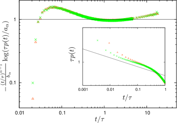
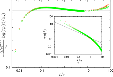
These observations are confirmed by plotting $-\frac{{t/\tau}^{\alpha-1}}{b_{\alpha}}\log(\tau p(t)/a_{\alpha})$ against $t/\tau$. If the proposed form of a stretched exponential is correct, then the numerical curves should approach a constant asymptotically Altmann and Kantz (2005). The main plots in Figs. 7,8 show the results for $\alpha=0.2,0.7$. The numerical curves bend around the horizontal line, suggesting that a stretched exponential is too simplistic to describe the functional form of the asymptote. We find that the agreement with the ansatz improves with increasing $\alpha$. For the most part, the dependence on series length is weak for the series we considered.

The particularly strong deviations from the proposed stretched exponential given in Eq. (17) for $t<\tau$ have also been observed for other stationary long-range correlated series Eichner et al. (2007). The authors conjecture that instead the initial asymptote rather follows a power law with slope $-\alpha$. We test this hypothesis in the insets of Figs. 7,8 for $\alpha=0.2,0.7$ respectively. The agreement with the power-law ansatz is reasonable and improves with decreasing $\alpha$ and increasing quantile.

Figure 7: (Color online) Main plot: distribution of return times above the $99.7\%$ quantile for sequences of lengths $2^{19},2^{21}$ (triangles, crosses) for $\alpha=0.2$. Inset: distribution of return times above the $99.1\%,99.7\%$ quantiles (triangles, crosses) for sequences of length $2^{21}$ and $\alpha=0.2$. A power law with slope $-\alpha$ is plotted alongside.

Figure 8: (Color online) Main plot: distribution of return times above the $99.7\%$ quantile for sequences of lengths $2^{19},2^{21}$ (triangles, crosses) for $\alpha=0.7$. Inset: distribution of return times above the $99.1\%,99.7\%$ quantiles (triangles, crosses) for sequences of length $2^{21}$ and $\alpha=0.7$. A power law with slope $-\alpha$ is plotted alongside.

To summarize, while it is still possible that the ansatz for the return time distribution of stationary long-range correlated series given in Eq. (17) generally holds for $t>\tau$ in the limit of infinitely long time series, there are significant deviations from it for the long but finite time series considered here. These deviations also depend on the threshold in a counter-intuitive way such that the deviations are stronger for higher thresholds.

V Conclusion

Long-range correlated series with an underlying distribution belonging to the Weibull class of extreme values have received little attention in the literature. We believe that our study will be of relevance to certain quantities that approach finite bounds sufficiently slowly (for a precise mathematical statement, see de Haan and Ferreira (2006)). Possible examples include humidity NREL (1993), strength of materials Weibull (1951), and critical path analysis Thornley (2001). In the latter case, the beta distribution is often used for modelling completion times of activities.

While in the mathematical literature one can find important extensions of iid extreme value statistics to stationary dependent series Leadbetter et al. (1983); Leadbetter and Rootzén (1988), we have focussed on extremal quantities that are measured with respect to a reference point that is itself a random variable. Apart from the mathematical interest, this is motivated by practical applications. To pick just one of the examples, the maximum relative to the minimum gives a measure of the full range traversed by a trajectory in a stochastic process. In many cases, the distribution of the reference point dominates or convolves with the distribution of the extremes giving rise to extremal distributions very different from the Weibull distribution. Moreover, we found that the extremal distributions in the correlated stationary series converge to their iid counterparts for the specific processes considered.

While it was proposed that the form of return interval distributions in correlated stationary series asymptotically approaches a stretched exponential for large return intervals independent of the underlying distribution Eichner et al. (2007), our results for the uniform and beta distribution do not support this. Although a stretched exponential is appealing and fully-determined once $\alpha$ has been estimated, we believe that this can only be a first approximation. However, a power-law decay with slope $-\alpha$ for short return intervals is more convincing. Together with the results presented in Ref. Eichner et al. (2007), this suggests that this behavior might be universal and independent of the underlying distribution.

VI Appendix

The numerical results presented in this article are based on an algorithm proposed in Refs. Schreiber and Schmitz (1996, 2000) to generate realizations of stochastic processes with a desired PDF and desired correlations. While the algorithm has been extensively tested and is well-established, questions remain as to the nature of the sample paths, the step size distribution, etc. To investigate these points, we apply the algorithm to the case of a uniform PDF with $\alpha=2$, which should correspond to a diffusion-like process. This is indeed what we find.

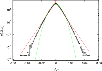
In Fig. 9 we plot the distribution of the step sizes between successive points in series of length $32768$ and $\alpha=2$. The distribution lies somewhere between a Gaussian and a symmetric exponential, i.e. distributions with suppressed tails (as opposed to, say, power-law tails arising from an underlying Lévy motion).

Figure 9: (Color online) Distribution of step sizes for series of length $32768$ and $\alpha=2$. A Gaussian and a symmetric exponential, both with the same standard deviation as the data, have been plotted alongside as solid lines.

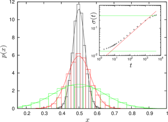
To minimize the effect of the finite support of the uniform distribution, we also studied the time evolution of those realizations or series beginning in the middle of the interval. The inset of Fig. 10 plots the standard deviation of the distribution of these series as a function of time. Numerically, among our ensemble of series we included all those that began with values in the narrow interval $0.475\leq x\leq 0.525$. Since the random variables are drawn from a uniform distribution, at time $t=0$ their distribution has standard deviation $\sigma(t=0)=\sqrt{3}/120$, which is indicated by the lower horizontal line. For intermediate times the distribution spreads with a standard deviation $\sigma(t)\propto\sqrt{t}$. For long times the distribution crosses over to a uniform spread across the interval, as indicated by the upper horizontal line with standard deviation $\sigma(t\to\infty)=\sqrt{3}/6$. This is consistent with diffusion. However, an idiosynchracy of the Schreiber-Schmitz method is that the possible values encountered in the series are quenched at time $t=0$. Therefore, preselected realizations starting in the middle narrow interval exhaust a fraction of the uniform deviates from this region of the $[0,1]$ interval and, correspondingly, a relatively larger amount of values is subsequently encountered around the endpoints. This is the reason for the overshoot of the standard deviation past the upper horizontal line, since the distribution is slightly enhanced at its endpoints (and slightly diminished around $0.5$) with respect to a uniform distribution. But after all the values in the series have been accounted for, the distribution of the original uniform draw is recovered. Fig. 10 illustrates that, for intermediate times, the evolving distributions are well approximated by Gaussians, as expected for diffusion.

Figure 10: (Color online) Time evolution of the PDF for sequences initially starting within $0.475\leq x\leq 0.525$ after $25,100,500$ steps (top to bottom), for $L=32768$ and $\alpha=2$. Gaussians with the same standard deviation as the data are plotted alongside. Inset: Time evolution of the standard deviation of the PDF (crosses) for sequences initially starting within $0.475\leq x\leq 0.525$. The standard deviations of the initial and final uniform distributions are $\sqrt{3}/120$ and $\sqrt{3}/6$ (horizontal lines), respectively. For a range of intermediate times the standard deviation grows with the square root of the number of steps (diagonal line).

References

- Bechhoefer and Marshall (2007) J. Bechhoefer and B. Marshall, Phys. Rev. Lett. 98, 098105 (2007).
- Majumdar and Krapivsky (2000) S. N. Majumdar and P. L. Krapivsky, Phys. Rev. E 62, 7735 (2000).
- Ben-Naim et al. (2001) E. Ben-Naim, P. L. Krapivsky, and S. N. Majumdar, Phys. Rev. E 64, 035101(R) (2001).
- Majumdar and Krapivsky (2002) S. N. Majumdar and P. L. Krapivsky, Phys. Rev. E 65, 036127 (2002).
- Bouchaud and Mézard (1997) J. P. Bouchaud and M. Mézard, J. Phys. A: Math. Gen. 30, 7997 (1997).
- Biroli et al. (2007) G. Biroli, J. P. Bouchaud, and M. Potters, J. Stat. Mech. p. P07019 (2007).
- Muzy et al. (2006) J. F. Muzy, E. Bacry, and A. Kozhemyak, Phys. Rev. E 73, 066114 (2006).
- Bunde et al. (2002) A. Bunde, J. Kropp, and H. J. Schellnhuber, eds., The Science of Disasters – Climate Disruptions, Heart Attacks, and Market Crashes (Springer, Berlin, 2002).
- Battjes and Gerritsen (2002) J. A. Battjes and H. Gerritsen, Phil. Trans. R. Soc. Lond. A 360, 1461 (2002).
- Leadbetter et al. (1983) M. R. Leadbetter, G. Lindgren, and H. Rootzén, Extremes and Related Properties of Random Sequences and Processes (Springer-Verlag, New York, Heidelberg, Berlin, 1983).
- Leadbetter and Rootzén (1988) M. R. Leadbetter and H. Rootzén, Ann. Probab. 16, 431 (1988).
- Sethna et al. (2001) J. P. Sethna, K. A. Dahmen, and C. R. Myers, Nature (London) 410, 242 (2001).
- Hurst (1951) H. E. Hurst, Transaction of the American Society of Civil Engineers 116, 770 (1951).
- Monetti et al. (2003) R. A. Monetti, S. Havlin, and A. Bunde, Physica A 320, 581 (2003).
- Pelletier and Turcotte (1997) J. Pelletier and D. L. Turcotte, Journal of Hydrology 203, 198 (1997).
- Huybers and Curry (2006) P. Huybers and W. Curry, Nature (London) 441, 329 (2006).
- Majumdar and Comtet (2004) S. N. Majumdar and A. Comtet, Phys. Rev. Lett. 92, 225501 (2004).
- Györgyi et al. (2007) G. Györgyi, N. R. Moloney, K. Ozogány, and Z. Rácz, Phys. Rev. E 75, 021123 (2007).
- Burkhardt et al. (2007) T. W. Burkhardt, G. Györgyi, N. R. Moloney, and Z. Rácz, Phys. Rev. E 76, 041119 (2007).
- Cox and Isham (1980) D. R. Cox and V. Isham, Point Processes (Chapman and Hall, London and New York, 1980).
- Corral (2004) A. Corral, Phys. Rev. Lett. 92, 108501 (2004).
- Davidsen et al. (2007) J. Davidsen, S. Stanchits, and G. Dresen, Phys. Rev. Lett. 98, 125502 (2007).
- Baiesi et al. (2006) M. Baiesi, M. Paczuski, and A. L. Stella, Physical Review Letters 96, 051103 (2006).
- Bunde et al. (2005) A. Bunde, J. F. Eichner, J. W. Kantelhardt, and S. Havlin, Phys. Rev. Lett. 94, 048701 (2005).
- Vázquez et al. (2006) A. Vázquez, J. G. Oliveira, Z. Dezsö, K. I. Goh, I. Kondor, and A. L. Barabási, Phys. Rev. E 73, 036127 (2006).
- Altmann and Kantz (2005) E. G. Altmann and H. Kantz, Phys. Rev. E 71, 056106 (2005).
- Eichner et al. (2007) J. F. Eichner, J. W. Kantelhardt, A. Bunde, and S. Havlin, Phys. Rev. E 75, 011128 (2007).
- Corral (2005) A. Corral, Phys. Rev. Lett. 95, 028501 (2005).
- Sornette et al. (2008) D. Sornette, S. Utkin, and A. Saichev, Phys. Rev. E 77, 066109 (2008).
- Santhanam and Kantz (2008) M. S. Santhanam and H. Kantz, Phys. Rev. E 78, 051113 (2008).
- de Haan and Ferreira (2006) L. de Haan and A. Ferreira, Extreme Value Theory: An Introduction (Springer, New York, 2006).
- Raychaudhuri et al. (2001) S. Raychaudhuri, M. Cranston, C. Przybyla, and Y. Shapir, Phys. Rev. Lett. 87, 136101 (2001).
- Sabhapandit and Majumdar (2007) S. Sabhapandit and S. N. Majumdar, Phys. Rev. Lett. 98, 140201 (2007).
- Hnat et al. (2002) B. Hnat, S. C. Chapman, G. Rowlands, N. W. Watkins, and M. P. Freeman, Geophys. Res. Lett. 29, 35 (2002).
- Schreiber and Schmitz (1996) T. Schreiber and A. Schmitz, Phys. Rev. Lett. 77, 635 (1996).
- Schreiber and Schmitz (2000) T. Schreiber and A. Schmitz, Physica D 142, 346 (2000).
- Györgyi et al. (2008) G. Györgyi, N. R. Moloney, K. Ozogány, and Z. Rácz, Phys. Rev. Lett. 100, 210601 (2008).
- Berman (1964) S. M. Berman, Ann. Math. Stat. 35, 502 (1964).
- Bouchaud and Georges (1990) J. P. Bouchaud and A. Georges, Phys. Rept. 195, 127 (1990).
- Ibragimov and Linnik (1971) I. A. Ibragimov and Y. V. Linnik, Independent and stationary sequences of random variables (Wolters-Noordhoff Publishing, Groningen, 1971).
- Coles (2001) S. Coles, An introduction to statistical modeling of extreme values (Springer-Verlag, London, 2001).
- (42) We simulated long-range correlated processes with based on the beta distribution for , , and , .
- NREL (1993) NREL, Solar and meteorological surface observation network (U.S. Department of Energy, National Renewable Energy Laboratory, Golden, CO, 1993).
- Weibull (1951) W. Weibull, J. Appl. Mech. 18, 293 (1951).
- Thornley (2001) G. Thornley, ed., Critical Path Analysis in Practice (Routledge, 2001).