Stability of a growth process generated by monomer filling with nearest-neighbour cooperative effects

Abstract

We study stability of a growth process generated by sequential adsorption of particles on a one-dimensional lattice torus, that is, the process formed by the numbers of adsorbed particles at lattice sites, called heights. Here the stability of process, loosely speaking, means that its components grow at approximately the same rate. To assess stability quantitatively, we investigate the stochastic process formed by differences of heights.

The model can be regarded as a variant of a Pólya urn scheme with local geometric interaction.

Keywords: Cooperative sequential adsorption, deposition, growth, urn models, reinforced random walks, Lyapunov function.

Subject classification: primary 60G17, 62M30; secondary 60J20.

1 Introduction

1.1 The model and results

Let $\{1,2,\ldots,N+1\}$ be a lattice segment with periodic boundary conditions, i.e. a one dimensional lattice torus with $N+1$ points. Assume that $N\geq 2$. The growth process is a discrete-time Markov chain $\xi(t)=(\xi_{1}(t),\ldots,\xi_{N+1}(t)),\,t\in\mathbb{Z}_{+}=\{0,1,2,\dots\}$ with values in $\mathbb{Z}_{+}^{N+1}$, specified by the following transition probabilities:

$${\mathbb{P}}\{\xi_{i}(t+1)=\xi_{i}(t)+1,\ \xi_{j}(t+1)=\xi_{j}(t)\ \forall j\neq i\,|\,\xi(t)\}=\frac{\beta^{u_{i}(t)}}{\sum_{j=1}^{N+1}\beta^{u_{j}(t)}},$$

$$u_{i}(t)=\sum\limits_{j\in U_{i}}\xi_{j}(t),\ \ i=1,2,\dots,N+1,$$

where $\beta>0$ and $U_{i}$ is a certain neighbourhood of site $i$.

Definition 1

The quantity $u_{i}(t)$ is called a potential of site $i$ at time $t$.

We consider the following three possibilities for neighbourhood $U_{i}$:

• : $U_{i}=\{i\}$, no interaction;

• : $U_{i}=\{i,i+1\}$, asymmetric interaction;

• : $U_{i}=\{i-1,i,i+1\}$, symmetric interaction,

where $U_{N+1}=\{N+1,1\}$ due to periodic boundary conditions in case (A2); similarly $U_{1}=\{N+1,1,2\},\,U_{N+1}=\{N,N+1,1\}$ in case (A3). It should be noted that periodic boundary conditions are imposed for technical reasons only to avoid boundary effects.

The growth process above describes random sequential allocation of particles at the lattice sites, where $\xi_{k}(t)$ is the number of particles at site $k$ at time $t$. It is motivated by cooperative sequential adsorption (CSA) model widely used in physics and chemistry for representation of adsorption processes. CSA is probabilistic in nature and captures the following important feature of adsorption processes. A molecule diffusing around a certain material surface (say, a bounded region either of continuous space or lattice) might get adsorbed by the surface. The adsorption probability depends on a spatial configuration formed by locations of previously adsorbed particles; for example, the subsequent particles are more likely to get adsorbed around locations of previously adsorbed particles. In the opposite scenario the adsorbed particles can inhibit adsorption in their neighbourhoods. For additional details and examples we refer the reader to [2, 16] and references therein.

The model under consideration relates to a version of CSA where the unnormalized adsorption probability at a location depends on the number of particles previously adsorbed in its neighbourhood. In the mostly studied in physics adsorption model, namely, random sequential adsorption (RSA), the adsorption probability equals $0$ at any location with one or more neighbours and equals $1$ otherwise, i.e. essentially no neighbours are allowed. Asymptotic and statistical studies of CSA generalizing RSA (by allowing any number of neighbours) were undertaken in [15, 19]; see also [20], where one proposes a model of point process motivated by this CSA.

Our model can also be regarded as a one-dimensional lattice variant of CSA described in [14], where the adsorbing probability takes the form of a product of probabilities associated with each of the adsorbed nearby particles. Indeed, in our model all neighbours contribute the same factor $\beta>0$ to the product, so that only the number of neighbours is relevant. If $\beta<1$, then one expects that adsorption slows down in a saturated region.

Another source of motivation has been provided by monomer filling with nearest-neighbour cooperative effects, see p.1289 of [2]. This is a continuous-time model on the lattice with a hard-core type constraint: only a single particle can be adsorbed at a site. A site’s neighbourhood is understood as usual, i.e. as in our case (A3), and the intensity of adsorption at a site depends on the number of existing neighbours. As a result, there are three non-zero intensities: $\lambda_{0},\lambda_{1}$ and $\lambda_{2}$, determining the model dynamics in the one-dimensional case. The main difference of our model from monomer filling is that we allow any number of particles to be deposited at a site.

The infinite capacity assumption puts our model also into the usual “balls and bins” framework of urn models, see [11], with an essential difference resulting form additional interaction between bins. It is easy to see that in case (A1) the model is a particular variant of the well-known Pólya urn model (see a detailed discussion in Section 1.2).

Finally, we note that our model in case (A1) is closely related to models of neuron growth in biology, in particular to the one considered in [6] representing the early stage of neuron growth. In their model probability of adsorption is proportional to the $\alpha$-th power of the number of particles at a node ($u_{i}^{\alpha}(t)$ was used there instead of $\beta^{u_{i}(t)}$ in our paper). The same model with polynomial weights and its generalizations have been extensively used in modelling a so-called “positive feedback” in economics (e.g., see [9, 10] and references therein). A special limit variant of our model in case (A3) (arising as $\beta\rightarrow 0$, see Section 1.2) relates to the models of biological neural networks studied in [5, 7].

1.2 Stability

Loosely speaking, stability of the growth process means that the “profile” $\xi_{i}(t),\,i=1,\ldots,N+1$, is “approximately flat”, i.e. there are no extraordinary peaks. To describe this property in a formal way we introduce a process of differences $\zeta(t)=(\zeta_{1}(t),\ldots,\zeta_{N}(t))\in\mathbb{Z}^{N},\,t\in\mathbb{Z}_{+},$ where

$$\zeta_{i}(t)=\xi_{i}(t)-\xi_{N+1}(t),\,\,i=1,\ldots,N$$

and also for convenience set $\zeta_{N+1}(t)\equiv 0$. It is easy to see that $(\zeta(t),\,t\in\mathbb{Z}_{+})$ is also a Markov chain with the following transition probabilities

$${\mathbb{P}}\{\zeta_{i}(t+1)=\zeta_{i}(t)+\delta_{i,k},\ i=1,2,\dots,N\,|\,\zeta(t)\}=\frac{\beta^{\sum_{j\in U_{k}}\zeta_{j}(t)}}{Z(\zeta(t))}$$

and

$${\mathbb{P}}\{\zeta_{i}(t+1)=\zeta_{i}(t)-1,\ i=1,2,\dots,N\,|\,\zeta(t)\}=\frac{\beta^{\sum_{j\in U_{N+1}}\zeta_{j}(t)}}{Z(\zeta(t))},$$

where

$$Z(\zeta(t))=\sum\limits_{k=1}^{N+1}\beta^{\sum_{j\in U_{k}}\zeta_{j}(t)}.$$

and

$$\delta_{i,k} =\left\{\begin{array}[]{rcl}1,&\text{if}&i=k,\\ 0,&&\text{otherwise.}\end{array}\right.$$

Definition 2

We say that the growth process is stable if the process of differences is an ergodic (positive recurrent) Markov chain. Otherwise the growth process is called unstable.

The following arguments apply when $U_{i}=\{i\}$, when our model becomes a particular case of generalized Pólya urn model (see [6, 11]). Let $\xi_{i}(t),\,i=1,\dots,N+1,$ represent the numbers of the balls of $N+1$ different types at time $t$; the probability to pick a ball of a certain type $i$ is proportional to $w(\xi_{i}(t))$, and here $w(x)=\beta^{x}$. By Rubin’s construction arguments (see [1], Section 5) if

$$A_{i}=\left\{\lim_{t\to\infty}\xi_{i}(t)=\infty,\ \sup_{t}\xi_{j}(t)<\infty\ \text{ for all }j\neq i\right\},\quad i=1,\ldots,N+1,$$

and $\sum_{k=1}^{\infty}w(k)^{-1}<\infty$, then

$${\mathbb{P}}\left(\bigcup_{i=1}^{N+1}A_{i}\right)=1.$$

Applying the result to our model with $\beta>1$, since $\zeta_{i}(t)=\xi_{i}(t)-\xi_{N+1}(t)$, we obtain that either $\zeta_{i}(t)\to\infty$ for some $i\in\{1,\dots,N\}$ (on event $A_{i}$), or all $\zeta_{i}(t)\to-\infty$ (on event $A_{N+1}$). In both cases transience of the process of differences follows. Thus, the general result for the urn model implies that the growth process is unstable.

In the opposite situation, i.e. when $\sum_{k=1}^{\infty}w(k)^{-1}=\infty$, Rubin’s results imply that with probability $1$ all components of the growth process grow to infinity and this is the case in our model with $0<\beta\leq 1$. We prove a stronger result in the case $0<\beta<1$, namely, we show that the distribution of the process of differences stabilizes, i.e. converges to a stationary distribution.

If $\beta=1$, then, regardless of the type of neighbourhood, with probability $1$ all components of the process grow to infinity, but the growth is unstable. Indeed, in this case the process of differences is a zero drift spatially homogenous random walk with bounded jumps which asymptotic behaviour is well-known (Theorem 8.1, ch. 2, in [18]). If $N\geq 3$, then the random walk is transient. If $N=2$, then the random walk is recurrent, but it is null recurrence (as follows from the subsequent arguments), therefore the growth is unstable for $N=2$ as well. If, just for this instance, we also allow $N=1$ (since the process is well-defined in this case as well), then the process of differences is just a one-dimensional simple symmetric random walk, which is non-ergodic. If $N=2$, then null recurrence of the random walk follows from null recurrence of its coordinates, since each of them is just a one-dimensional symmetric random walk. Thus in the case $\beta=1$ instability is implied by the properties of zero-drift random walks, therefore this case is completely eliminated from our further considerations.

Stability of the growth process is rather intuitive in the no-interaction case, i.e. $U_{i}=\{i\}$, if $0<\beta<1$. Indeed, in this case growth slows down at the sites with the maximal potential and accelerates at the sites with the minimal potential resulting in the stability effect, in contrast to the case $\beta>1$ where growth accelerates at the sites with the maximal potential and no stability is observed. The picture is not so straightforward for the models with interaction: for instance, it turns out that the growth process is unstable for the model with symmetric interaction for any value of $\beta$.

To understand possible sources of instability in the models with interaction it is helpful to consider two other growth processes, which can be viewed as “extreme” versions of our growth process resulted from letting $\beta\rightarrow 0$ and $\beta\rightarrow\infty$ respectively.

An easy calculation shows that as $\beta\rightarrow 0$ the probability to get adsorbed not at one of the minima converges to $0$. Therefore, a natural interpretation of the formal case “$\beta=0$” is that at time $t+1$ a particle is allocated equally likely at any site $i$ such that $u_{i}(t)=\min_{k=1,\ldots,N+1}u_{k}(t)$. Similarly, “$\beta=\infty$” can be interpreted as the situation when at time $t+1$ a particle is allocated equally likely at any site $i$ such that $u_{i}(t)=\max_{k=1,\ldots,N+1}u_{k}(t)$. Consider, for instance, the case $\beta=0$, $N+1=4$, and $U_{i}=\{i-1,i,i+1\}$. It is easy to see that, depending on the initial configuration, with probability $1$ one of the two following events occur: the growth is at even nodes only, the growth is at odd nodes only. Such limit configurations can be called an attractor of the process by analogy with similar phenomena observed in probabilistic models of biological neural networks (see [5, 7] for details). If $N$ is arbitrary, then it is also possible to describe all limit configurations of the growth processes in both “$\beta=0$” and “$\beta=\infty$” cases. The case “$\beta=\infty$” is trivial regardless of the value of $N$ and the type of interaction. On the other hand, the limit behaviour of the growth process corresponding to “$\beta=0$” is non-trivial in case of an arbitrary $N$ for both asymmetric and symmetric interaction, despite quite limited randomness of the process dynamics. A detailed study of these extreme models is presented in [21].

Though our study of stability of the growth process relates also to the study of morphology of random interfaces of growing materials generated by ballistic deposition processes (e.g., see [12, 13] and references therein), both our setup and the methodology are quite different from the ones used in the present paper, therefore we do not investigate this analogy in further details.

1.3 Results

Here and further in the paper by transience of the process $\zeta(t)=(\zeta_{1}(t),\dots,\zeta_{N}(t))$ we understand $\lim_{t\to\infty}|\zeta(t)|\to\infty$, where $|\cdot|$ is the usual Euclidean norm.

Theorem 1

Suppose $U_{i}=\{i\},\,i=1,\ldots,N+1$.

• If $0<\beta<1$, then Markov chain $(\zeta(t),\,t\in\mathbb{Z}_{+})$ is ergodic.

• If $\beta>1$, then Markov chain $(\zeta(t),\,t\in\mathbb{Z}_{+})$ is transient.

The assertion of the second part of Theorem 1 is a corollary of the well known results for Pólya urn scheme, see [9, 10], and also the discussion in Section 1.2.

Before we formulate the next statement, we need the following definition.

Definition 3

Consider a planar process $\zeta(t)$ with polar coordinates $({\bf r}(t),\varphi(t))$, $t\geq 0$. We say that $\zeta$ is essentially a clockwise spiral, if

• $|{\bf r}(t)|\to\infty$ as $t\to\infty$, and

• for some large enough time $\tau_{0}$ such that $\varphi(\tau_{0})=2\pi k_{0}$ where $k_{0}\in\mathbb{Z}$ we have we have

  $$\varphi(\tau_{n})=2\pi k_{0}+\frac{\pi n}{2},\ \ \text{ for all }n=0,1,2,\dots,$$

  where all

  $$\tau_{n}=\inf\{t>\tau_{n-1}:\varphi(t)=\frac{\pi k}{2}\text{ for some }k\in\mathbb{Z}\},\ \ n=1,2,\dots$$

  are finite.

Theorem 2

Suppose $U_{i}=\{i,i+1\},\,i=1,\ldots,N+1$.

• If $N=2$ and $0<\beta<1$, then Markov chain $(\zeta(t),\,t\in\mathbb{Z}_{+})$ is ergodic. Consequently, $\xi_{1}(t)=\xi_{2}(t)=\xi_{3}(t)$ for infinitely many $t$’s almost surely.

• If $\beta>1$, then Markov chain $(\zeta(t),\,t\in\mathbb{Z}_{+})$ is transient. Moreover, if also $N=2$, then the trajectory of $(\zeta_{1}(t),\zeta_{2}(t))$ is essentially a clockwise spiral, and $\xi_{1}(t)=\xi_{2}(t)=\xi_{3}(t)$ only for finitely many $t$’s a.s.

It should be noted that when $N=2$ there is an interesting comparison between Theorem 2 on the one hand, and the Friedman urn on the other hand. There will be infinitely many “ties” ($\xi_{k}(1)=\xi_{k}(2)=\xi_{k}(3)$ for infinitely many $k$’s) if $\beta<1$; in a Friedman urn with $\rho<1/2$ there will be infinitely many ties, while the opposite occurs when $\rho>1/2$: see [4] and Section 6 in [8].

Theorem 3

Suppose $U_{i}=\{i-1,i,i+1\},\,i=1,\ldots,N+1$. Then Markov chain $(\zeta(t),\,t\in\mathbb{Z}_{+})$ is transient for any $N\geq 3$ for any $\beta\in(0,1)\cup(1,\infty)$. Moreover, if $\beta>1$, then with probability $1$ there is a $k\in\{1,\dots,N+1\}$ such that

$$\lim_{t\to\infty}\xi_{i}(t) =\infty,\text{ if and only if }i\in\{k-1,k\},\mbox{ and}$$

$$\lim_{t\to\infty}\frac{\xi_{k}(t)}{\xi_{k-1}(t)} =\beta^{c},$$

where $c=\lim_{t\to\infty}[\xi_{k+1}(t)-\xi_{k-2}(t)]\in\mathbb{Z}$.

To prove the results of the present paper we combine the constructive methods of studying asymptotic behaviour of countable Markov chains from [3] with probabilistic techniques used in the theory of processes with reinforcement from [22] (in contrast with the purely combinatorial methods used in [21]).

2 Proofs

2.1 Proof of Theorem 1

If $U_{i}=\{i\}$, then process of differences $(\zeta_{t},\,t\in\mathbb{Z}_{+})$ has the transition probabilities

$${\mathbb{P}}\{\zeta_{i}(t+1)=\zeta_{i}(t)+\delta_{i,k},\ \forall i\,|\,\zeta(t)\}=\frac{\beta^{\zeta_{k}(t)}}{1+\sum_{j=1}^{N}\beta^{\zeta_{j}(t)}},\quad k=1,\ldots,N,$$

and

$${\mathbb{P}}\{\zeta_{i}(t+1)=\zeta_{i}(t)-1,\,i=1,\ldots,N\,|\,\zeta(t)\}=\frac{1}{1+\sum_{j=1}^{N}\beta^{\zeta_{j}(t)}}$$

Suppose $0<\beta<1$. Consider the following function

$$f({\bf x})=|{\bf x}|^{2}=\sum\limits_{i=1}^{N}x_{i}^{2},\quad{\bf x}=(x_{1},\ldots,x_{N})\in\mathbb{Z}^{N}.$$

It is easy to see that

$$\Delta:={\mathbb{E\,}}[f(\zeta(t+1))-f(\zeta(t))\,|\,\zeta_{t}={\bf x}]=\frac{\sum_{i=1}^{N}\left(2x_{i}(\beta^{x_{i}}-1)+1+\beta^{x_{i}}\right)}{1+\sum_{i=1}^{N}\beta^{x_{i}}},$$

and for any $\varepsilon>0$

$$\Delta+\varepsilon=\frac{\varepsilon-\sum_{i=1}^{N}(2x_{i}(1-\beta^{x_{i}})-1-(\varepsilon+1)\beta^{x_{i}})}{1+\sum_{i=1}^{N}\beta^{x_{i}}}.$$

Now let

$$h(x)=2x(1-\beta^{x})-1-(\varepsilon+1)\beta^{x}.$$

It is clear that for $x>0$ sufficiently large, $h(x)\sim 2x$, formally, there is an $A^{\prime}>0$ such that for $x\geq A^{\prime}$ we have $h(x)\geq x$. Conversely, when $x=-a<0$,

$$h(x)=h(-a)=\frac{1}{\beta^{a}}(2a-\varepsilon-1)-1-2a.$$

so that $h(-a)$ grows approximately exponentially and again there is an $A^{\prime\prime}>0$ such that $h(-a)\geq a$ when $a\geq A^{\prime\prime}$. Now set

$$-C:=\inf_{x\in(-A^{\prime},A^{\prime})}(h(x)-|x|)=\inf_{x\in{\mathbb{R}}}(h(x)-|x|)$$

(note that $\varepsilon+2\leq C<\infty$). Consequently,

$$\sum_{i=1}^{N}(2x_{i}(1-\beta^{x_{i}})-1-(\varepsilon+1)\beta^{x_{i}}) =\sum_{i=1}^{N}h(x_{i})=\sum_{i=1}^{N}|x_{i}|+\sum_{i=1}^{N}\left(h(x_{i})-|x_{i}|\right)$$

$$\geq\sum_{i=1}^{N}|x_{i}|-CN$$

Therefore,

$$\Delta+\varepsilon\leq\frac{CN+\varepsilon-\sum_{i=1}^{N}|x_{i}|}{1+\sum_{i=1}^{N}\beta^{x_{i}}}\leq 0$$

except for a possibly finite number of $(x_{1},\dots,x_{N})$ lying in the “bad” set

$$M:=\left\{\sum_{i=1}^{N}|x_{i}|\leq CN+\varepsilon\right\}.$$

Hence, the conditions of the Foster criterion (Theorem 5) are satisfied and Markov chain $(\zeta(t),\,t\in\mathbb{Z}_{+})$ is ergodic. Thus the first part of Theorem 1 is now proved.  

2.2 Proof of Theorem 2

2.2.1 Proof of part (1) of Theorem 2

Let $N=2$ and $0<\beta<1$. Set $\zeta_{1}(t)=\xi_{1}(t)-\xi_{3}(t)$ and $\zeta_{2}(t)=\xi_{2}(t)-\xi_{3}(t)$. The new process $\zeta(t)=(\zeta_{1}(t),\zeta_{2}(t))$ is a time-homogeneous Markov chain on $\mathbb{Z}^{2}$ with the following transitions

$${\mathbb{P}}\{\zeta(t)=(x_{1}+1,x_{2})|\zeta(t)=(x_{1},x_{2})\} =\frac{\beta^{x_{1}+x_{2}}}{\beta^{x_{1}+x_{2}}+\beta^{x_{2}}+\beta^{x_{1}}},$$

$${\mathbb{P}}\{\zeta(t)=(x_{1},x_{2}+1)|\zeta(t)=(x_{1},x_{2})\} =\frac{\beta^{x_{2}}}{\beta^{x_{1}+x_{2}}+\beta^{x_{2}}+\beta^{x_{1}}}$$

$${\mathbb{P}}\{\zeta(t)=(x_{1}-1,x_{2}-1)|\zeta(t)=(x_{1},x_{2})\} =\frac{\beta^{x_{1}}}{\beta^{x_{1}+x_{2}}+\beta^{x_{2}}+\beta^{x_{1}}}.$$

It is natural to expect that the Markov chain approximately follows the solutions of the differential equation

$$\frac{dx_{2}}{dx_{1}}=\frac{\beta^{x_{2}}-\beta^{x_{1}}}{\beta^{x_{1}+x_{2}}-\beta^{x_{1}}}$$

or, after making a substitution $u=\beta^{-x_{1}}$, $v=\beta^{-x_{2}}$,

$$\frac{dv}{du}=\frac{v(u-v)}{u(1-v)}$$ (2.1)

which we cannot solve analytically, but whose solutions seem to be spirals (see Figure 1). Hence a good candidate for a Lyapunov function for the process, i.e. the function $f({\bf x})=g(\beta^{-x_{1}},\beta^{-x_{2}})$ such that ${\mathbb{E\,}}[f(\zeta(t+1))-f(\zeta(t))\,|\,\zeta(t)={\bf x}]\leq-{\rm const}$ would be a function which level curves have a constant angle with the vector field generated by (2.1). Then the level curves for $g(u,v)$ will satisfy the differential equation

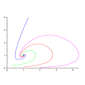
Figure 1: Trajectories of the dynamical process following the Markov chain.

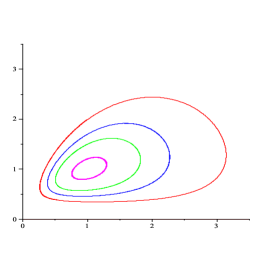
Figure 2: “Ideal” level curves.

$$\left(\frac{\partial g}{\partial u},\frac{\partial g}{\partial v}\right)\cdot\left[(v(v-u),u(1-v))\left(\begin{array}[]{cc}\cos\alpha&-\sin\alpha\\ \sin\alpha&\cos\alpha\end{array}\right)\right]=0$$

for some $\alpha$, which in turn might depend on initial conditions. Numerical solutions for the level curves are presented in Figure 2. Though not being able to solve the above equations analytically, we found an alternative suitable function (2.2), whose level curves are in Figure 3. Thus the proof of part (1) of Theorem 2 is based on the following lemma.

Lemma 1

Suppose that $\beta<1$. Let

$$f({\bf x})=\beta^{1-x_{1}-x_{2}}+\beta^{-3x_{1}+x_{2}}+\beta^{3x_{1}-4x_{2}}+\beta^{x_{1}+4x_{2}},$$ (2.2)

for any ${\bf x}=(x_{1},x_{2})$. Then for any $\delta>0$

$${\mathbb{E\,}}[f(\zeta(t+1))-f(\zeta(t))\,|\,\zeta(t)={\bf x}]\leq-(1-\beta)$$

once $|{\bf x}|\equiv\sqrt{x_{1}^{2}+x_{2}^{2}}$ is larger than some $C=C(\beta)>0$.

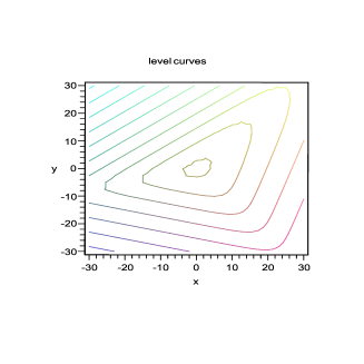
Figure 3: Level curves for $f(x,y)$ given in (2.2) for $\beta=0.9$

Proof of Lemma 1. We see that

$${\mathbb{E\,}}[f(\zeta(t+1))-f(\zeta(t))\,|\,\zeta(t)={\bf x}]+1-\beta=-\frac{(1-\beta)A(u,v)}{\beta^{5}v^{4}u^{3}(1+u+uv)}$$ (2.3)

where

$$A(u,v) =(\beta^{7}+\beta^{6})v^{3}u^{3}+(\beta^{6}+\beta^{5})v^{5}u+(\beta^{8}+\beta^{5}+\beta^{6}+\beta^{7})v^{9}u^{4}$$

$$+[(\beta^{7}+\beta^{5}+\beta^{6})u-(\beta+\beta^{2}+\beta^{3}+\beta^{4})]vu^{6}+v^{6}\beta^{5}+\beta^{5}u^{7}$$

$$+\beta^{5}v^{9}u^{5}-\beta^{5}v^{4}u^{3}$$

$$-(1+u^{2}+uv+u^{2}v)u^{2}v^{4}\beta^{5}-(1+\beta+\beta^{2}+\beta^{3}+\beta^{4})u^{5}{v}^{8}-(\beta^{2}+\beta^{4}+\beta^{3})uv^{6}$$

and $u=\beta^{x_{1}}$, $v=\beta^{x_{2}}$. The term $\beta^{5}u^{5}v^{9}$ clearly dominates all the negative terms, and the term in the square brackets is nonnegative for $u$ sufficiently large, hence there is a constant $c_{1}$ such that $A(u,v)>0$ once $\min(u,v)\geq c_{1}$.

Similarly,

$$u^{7}A(1/u,v) =\beta^{5}u^{7}v^{6}+O(u^{6}v^{6})+(\beta^{8}+\beta^{5}+\beta^{6}+\beta^{7})v^{9}u^{3}+O(v^{9}u^{2})$$

which is also nonnegative once $\min(u,v)\geq c_{1}$ for some $c_{2}>0$ and

$$v^{9}A(u,1/v) =\beta^{5}u^{7}v^{9}+O(u^{7}v^{8})$$

is nonnegative when $\min(u,v)\geq c_{3}$ for some $c_{3}>0$.

Finally,

$$u^{7}v^{9}A(1/u,1/v) =\beta^{6}u^{6}v^{4}+\beta^{7}u^{4}v^{6}+(\beta^{5}+\beta^{6}+\beta^{7})v^{8}$$ (2.4)

$$+\beta^{5}v^{4}(v^{5}+u^{6}-[\beta^{-4}+\beta^{-3}+\beta^{-2}+\beta^{-1}]v^{4}u)$$

$$+\beta^{5}u^{4}v^{3}(\beta v^{3}+u^{3}-v^{2}u)+O(u^{6}v^{3})+O(u^{4}v^{5})$$

Let $K=\beta^{-4}+\beta^{-3}+\beta^{-2}+\beta^{-1}$. For $v\geq Ku$ the expression in the second line of (2.4) is always nonnegative; on the other hand for $u>K^{-1}v$ the term $u^{6}$ is going to dominate in this line, hence for $u,v$ larger than $K^{6}$ the second line of (2.4) is nonnegative. The third line of (2.4) is nonnegative when $u\geq v$. In principle, it can become negative when $u<v$, however, since $x$ and $y$ are integers, it implies that when $u<v$, also $u\leq\beta v$, so that $\beta v^{3}+u^{3}-v^{2}u>v^{2}(\beta v-u)\geq 0$. Thus we have established that $A(1/u,1/v)\geq 0$ for all legitimate $u,v$ such that $\min\{u,v\}\geq c_{4}$.

Consequently, we have shown that on the positive quadrant $A(u,v)\geq 0$ whenever

$$(u,v)\in[\varepsilon^{-1},\infty)\times[\varepsilon^{-1},\infty)\ \cup\ (0,\varepsilon]\times(0,\varepsilon]\ \cup\ (0,\varepsilon]\times[\varepsilon^{-1},\infty)\ \cup\ (\varepsilon^{-1},\infty)\times(0,\varepsilon]$$

for some $\varepsilon>0$ (assume without loss of generality that $\varepsilon<1$).

Next, since

$$A(u,v)=(v\beta^{5}+\beta^{5}+\beta^{7}v+\beta^{6}v)u^{7}+O(u^{6})$$

as a Taylor series on $u$ and

$$A(u,v)=u^{4}\beta^{5}(\beta^{3}+\beta^{2}+\beta+u+1)v^{9}+O(v^{8})$$

as a Taylor series on $v$, we see that there is an $\varepsilon_{1}\in(0,\varepsilon]$ such that for all $v\in[\varepsilon,\varepsilon^{-1}]$ and $u\geq\varepsilon_{1}^{-1}$, and for all $u\in[\varepsilon,\varepsilon^{-1}]$ and $v\geq\varepsilon_{1}^{-1}$ respectively, we have $A(u,v)\geq 0$.

On the other hand, for small $u$ and $v$ respectively, we have

$$A(u,v) =\beta^{5}v^{6}+u\times{\sf Polynom}_{1}(u,v,\beta)=\beta^{5}u^{7}+v\times{\sf Polynom}_{2}(u,v,\beta).$$

where ${\sf Polynom}_{i}(u,v,\beta)$, $i=1,2$, are some polynomial expressions involving $u$, $v$, and $\beta$. Hence there is an $\varepsilon_{2}\in(0,\varepsilon]$ such that $A(u,v)\geq 0$ whenever $0<u\leq\varepsilon_{2}$ and $v\in[\varepsilon,\varepsilon^{-1}]$ or $0<v\leq\varepsilon_{2}$ and $u\in[\varepsilon,\varepsilon^{-1}]$.

Combining all the results above, we conclude that the right side of (2.3) is nonnegative for all ${\bf x}\in\mathbb{Z}^{2}$ which are outside of the square $\left[-R,R\right]^{2}$ where $R=\log(\min\{\varepsilon_{1},\varepsilon_{2}\})/\log(\beta).$ Lemma 1 is proved.  

Because of Lemma 1 and the fact that $f({\bf x})\to\infty$ whenever $|{\bf x}|\to\infty$, we can apply Foster’s supermartingale criterion (Theorem 5).  

Remark 1

We observed that the following function

$$\tilde{f}({\bf x})=\max\left\{\frac{x_{1}+x_{2}}{10},\frac{8x_{1}-3x_{2}}{25},\frac{8x_{1}-7x_{2}}{20},\frac{-x_{1}-3x_{2}}{7}\right\}$$ (2.5)

also satisfies Foster’s supermartingale criterion (its level curves are congruent to the ones in Figure 4); however, the proof of this fact requires going through a large number of special cases and hence is omitted in favour of using (2.2).

Figure 4: Level curve for $\tilde{f}(x,y)$ given in (2.5).

2.3 Proof of part (2) of Theorem 2

We start by proving transience for any $N\geq 2$. Set $\eta_{i}(t)=\xi_{i}(t)-\xi_{i-1}(t),\,i=2,\ldots,N+1$ and $\eta_{1}(t)=\xi_{1}(t)-\xi_{N+1}(t)$, because of the periodic boundary conditions. Then

$$\xi_{1}(t) =\xi_{N+1}(t)+\eta_{1}(t),$$

$$\xi_{2}(t) =\xi_{N+1}(t)+\eta_{1}(t)+\eta_{2}(t),$$

$$\dots =\dots,$$

$$\xi_{N+1}(t) =\xi_{N+1}(t)+\eta_{1}(t)+\dots+\eta_{N+1}(t),$$

and obviously $\sum_{i=1}^{N+1}\eta_{i}(t)=0$. We also have

$${\mathbb{P}}\{\xi_{i}(t+1)=\xi_{i}(t)+1|\xi(t)\}\propto\beta^{2[\eta_{1}(t)+\dots+\eta_{i}(t)]+\eta_{i+1}(t)}$$

for $i\leq N$, and, in turn,

$$\xi_{i}(t+1)=\xi_{i}(t)+1\Leftrightarrow\left\{\begin{array}[]{rcl}\eta_{i}(t+1)&=&\eta_{i}(t)+1,\\ \eta_{i+1}(t+1)&=&\eta_{i+1}(t)-1.\end{array}\right\}$$

We are going to show that Markov chain

$$\eta(t)=\left(\eta_{1}(t),\eta_{2}(t),\dots,\eta_{N+1}(t)\right),\quad t\in\mathbb{Z}_{+},$$

with state space $\{{\bf x}=(x_{1},\dots,x_{N+1}):\ x_{1}+\dots+x_{N+1}=0\}$ is transient. It is easy to see that transience of $(\eta(t),t\in\mathbb{Z}_{+})$ implies transience of $(\zeta(t),t\in\mathbb{Z}_{+})$. Indeed, if $(\zeta(t),t\in\mathbb{Z}_{+})$ were recurrent, then $\xi_{1}(t)=\dots=\xi_{N+1}(t)$ for infinitely many $t$ almost surely. But this would imply that $\eta_{1}(t)=\dots=\eta_{N+1}(t)=0$ for infinitely many $t$ almost surely as well, thus contradicting its transience. In other words, coordinates of $\eta$-process are consecutive differences of coordinates of the growth process, therefore transience of $\eta(t)$ yields transience of the process of differences, because the probability distribution of the later does not depend on the subtracted coordinates (due to the symmetry and periodic boundary conditions).

To prove transience of $(\eta(t),t\in\mathbb{Z}_{+})$ we are going to apply Theorem 4. To this end, consider the function

$$f({\bf x})=\left\{\begin{array}[]{ll}1,&\text{ if }x_{1}=x_{2}=\dots=x_{N+1}=0\\ \\ \frac{\displaystyle 1}{\displaystyle\max\{|x_{1}|,|x_{2}|,\dots,|x_{N+1}|\}},&\text{ otherwise.}\end{array}\right.$$

defined for any ${\bf x}=(x_{1},\ldots,x_{N+1})$. We now will show that, provided that $|{\bf x}|$ is large enough, ${\mathbb{E\,}}[f(\eta(t+1))-f(\eta(t))\,|\,\eta(t)={\bf x}]\leq 0$, establishing the result.

Indeed, consider the four following possibilities.

• $N\geq 3$ and the maximum $L$ of $x_{1},x_{2},\dots,x_{N+1}$ is not unique and there are at least two indices $i,j$ such that $|x_{i}|=|x_{j}|=L$ and they are at least distance $2$ apart, i.e., $|i-j|\geq 2$ (understood with periodic boundary conditions).

• $N=2$ and $|x_{1}|=|x_{2}|=|x_{3}|=L$.

• The maximum $L$ is not unique and there are exactly two maximums next to each other.

• The maximum $L$ is unique.

Observe that in cases (a1) and (a2) no step of the chain $\eta$ can decrease the maximum, hence ${\mathbb{E\,}}[f(\eta(t+1))-f(\eta(t))\,|\,\eta(t)={\bf x}]\leq 0$ here.

In case (b) suppose without loss of generality that the maximum is achieved at nodes $2$ and $3$, so $|x_{2}|=|x_{3}|=L$. Then ${\mathbb{E\,}}[f(\eta(t+1))-f(\eta(t))\,|\,\eta(t)={\bf x}]$ is proportional (up to a positive coefficient) to

$$\beta^{2x_{1}+x_{2}}\left[\frac{1}{\max\{|x_{1}+1|,|x_{2}-1|,L\}}-\frac{1}{L}\right]$$

$$+\beta^{2x_{1}+2x_{2}+x_{3}}\left[\frac{1}{\max\{|x_{2}+1|,|x_{3}-1|\}}-\frac{1}{L}\right]$$

$$+\beta^{2x_{1}+2x_{2}+2x_{3}+x_{4}}\left[\frac{1}{\max\{L,|x_{3}+1|,|x_{4}-1|\}}-\frac{1}{L}\right]$$

(if $N=2$ then we set $x_{4}\equiv x_{1}$). We can see that unless $x_{3}=L=-x_{2}$ the quantity above is always negative. However, when $x_{3}=L=-x_{2}$ we also have that the quantity above is proportional to

$$\beta^{-x_{2}-x_{3}}\left[\frac{1}{L+1}-\frac{1}{L}\right]+\left[\frac{1}{L-1}-\frac{1}{L}\right]+\beta^{x_{3}+x_{4}}\left[\frac{1}{L+1}-\frac{1}{L}\right]$$

$$=\frac{2-(L-1)\beta^{x_{3}+x_{4}}}{L(L^{2}-1)}\leq\frac{2-(L-1)\beta}{L(L^{2}-1)}\ \text{\ (since $|x_{4}|\leq L-1\ \Rightarrow\ x_{3}+x_{4}\geq 1$)}$$

which is negative once $L\geq 3$.

Finally, in case (c) suppose that the maximum is achieved at node $2$, $|x_{2}|=L$. Then ${\mathbb{E\,}}[f(\eta(t+1))-f(\eta(t))\,|\,\eta(t)={\bf x}]$ is proportional to

$$(*):= \left[\frac{1}{\max\{|x_{1}+1|,|x_{2}-1|\}}-\frac{1}{L}\right]+\beta^{x_{2}+x_{3}}\left[\frac{1}{\max\{|x_{2}+1|,|x_{3}-1|\}}-\frac{1}{L}\right]$$

When $x_{2}=L$,

$$(*) =\left[\frac{1}{\max\{|x_{1}+1|,L-1\}}-\frac{1}{L}\right]+\beta^{x_{2}+x_{3}}\left[\frac{1}{L+1}-\frac{1}{L}\right]$$

$$\leq\frac{1}{L(L-1)}-\frac{\beta}{L(L+1)}\leq 0$$

once $L>(\beta+1)/(\beta-1)$.

And in the last subcase $x_{2}=-L$

$$(*) =\left[\frac{1}{L+1}-\frac{1}{L}\right]+\beta^{x_{2}+x_{3}}\left[\frac{1}{\max\{L-1,|x_{3}-1|\}}-\frac{1}{L}\right]$$

$$\leq-\frac{1}{L(L+1)}+\frac{\beta^{-1}}{L(L-1)}\leq 0$$

again once $L>(\beta+1)/(\beta-1)$.

Consequently, ${\mathbb{E\,}}[f(\eta(t+1))\,|\,\eta(t)={\bf x}]\leq f({\bf x})$ whenever $|{\bf x}|$ is sufficiently large, and by Theorem 4 Markov chain $(\eta(t),\,t\in\mathbb{Z}_{+})$ is transient. So the transience is proved for any $N\geq 2$.

From now on assume that $N=2$. First, let us prove that the process $\zeta(t)=(\zeta_{1}(t),\zeta_{2}(t))$ cannot remain indefinitely in either of the following $6$ areas: $x>y>0$, $y>x>0$, $x>0>y$, $y>0>x$, $0>y>x$, and $0>x>y$.

Indeed, suppose that for some time $t_{0}$ we have $\zeta(t_{0})\in\Psi_{1}:=\{(x,y)\in{\mathbb{R}}^{2}:x>y>0\}$. When $\zeta(t)\in\Psi_{1}$, it is clear that $\zeta_{2}(t)$ has the property ${\mathbb{E\,}}[\zeta_{2}(t+1)\,|\,\zeta(t)=(x,y)]\leq\zeta_{2}(t)$. Hence $M(t)=\zeta_{2}(t\wedge\tau)$, $t\geq t_{0}$, where

$$\tau:=\inf\{t>t_{0}:\ \zeta_{1}(t)=\zeta_{2}(t)\text{ or }\zeta_{2}(t)=0\}=\inf\{t>t_{0}:\zeta(t)\notin\Psi_{1}\}$$

is a non-negative supermartingale which converges a.s. Since $M(t+1)-M(t)$ takes only integer values, it means that for some (random) $T$, $M(t)=const$ for all $t\geq T$. However, this is impossible unless $\tau<\infty$, since for a fixed $y>0$ the probability

$${\mathbb{P}}(M(t+1)=M(t)-1\,|\,\zeta(t)=(x,y)\in\Psi_{1})=\frac{1}{1+\beta^{y}+\beta^{y-x}}>\frac{1}{2+\beta^{y}}$$

does not go to zero, thus implying by the conditional Borel-Cantelli lemma (see e.g. Corollary 2 on p. 518 in [17]) that for some large $t>T$ we have $M(t)\neq M(t+1)$. Therefore $\tau$ is finite.

When $\zeta(t_{0})\in\Psi_{2}:=\{(x,y)\in{\mathbb{R}}^{2}:y\geq x\geq 0\}$, set $M(t)=\zeta_{2}(\tau\wedge t)-\zeta_{1}(\tau\wedge t)$ and

$$\tau:=\inf\{t>t_{0}:\ \zeta_{1}(t)=\zeta_{2}(t)\text{ or }\zeta_{1}(t)=0\}.$$

Again $M(t)$ is a non-negative supermartingale which cannot converge unless $\tau<\infty$, since on $\{\tau=\infty\}$ the event $|M(t+1)-M(t)|<1$ implies $M(t+1)=M(k)$ and thus $\zeta_{1}(t+1)=\zeta_{1}(t)-1$.

The remaining $4$ cases will analyzed briefly, since the argument is very similar. When $x>0>y$ or $y>0>x$, the probability to go towards the axis $x=0$ is larger than away from it, hence eventually $\zeta(t)$ will leave either of these areas. When $0>y>x$ there is a drift upwards, and finally when $0>x>y$ there is a drift towards the line $x=y<0$ so that a non-negative supermartingale $\zeta_{1}(t)-\zeta_{1}(t)$ must converge, and at the same time $\zeta(t)$ cannot remain indefinitely on the line $(-a,-a-\Delta)$, where $\Delta>0$ is a constant and $a=i,i+1,i+2,\dots$, since along this line there is a non-diminishing probability to go up, of order $\beta^{-\Delta}$.

Finally, we need to show that the process $\zeta(t)$ eventually “rotates” in one direction on its way to infinity. This immediately follows from the following Lemma 2, taking into account the established transience, the Borel-Cantelli lemma and the summability in $a$ of the terms on the RHS of (2.6).  

Lemma 2

Assume $\beta>1$. Suppose $a,k\geq 1$ and let $E_{k}$ be the event $\{$the trajectory of $\zeta(t)$ for $t>k$ crosses $\{(0,y),y<0\}$, $\{(x,0),x<0\}$, $\{(0,y),y>0\}$, $\{(x,0),x\geq 0\}$ exactly in this order and ends up at point $(a^{\prime},0)$ with $a^{\prime}\geq a+1\}$. Then, for some $\nu=\nu(\beta)>0$ and all large $a>0$ we have

$${\mathbb{P}}\left(E_{k}^{c}\,|\,\zeta(k)=(a,0)\right)\ \leq\exp\left(-\nu a\right).$$ (2.6)

Also, similar statements hold for starting points $(0,-a)$, $(-a,0)$ and $(0,a)$.

Proof. (1) Let us show that when the process leaves $(a,0)$, it ends up at $(0,-b)$, $b\geq a$, with probability very close to $1$. This will be done by demonstrating that initially the process moves only right and left-down (south-west, SW for short), and then after reaching level $y=-a/2$ (for simplicity assume that $a$ is even), it moves only in the SW direction, all with high probability.

Indeed, suppose that $\zeta(\tau_{0})=(a,0)$ for some $\tau_{0}$. For $i=1,2,\dots$ define

$$\tau_{i} =\inf\{t:\ \zeta_{2}(t)=-i\},$$

$$A_{i} =\left\{\exists k\in\{1,\dots,a\}:\ \zeta_{2}(\tau_{i-1}+k)=-i,\text{ but }\zeta_{2}(\tau_{i-1}+m)=-i+1\ \forall m\in\{0,\dots,k-1\}\right\},$$

where the latter is the event that after reaching level $y=-(i-1)$, the process $\zeta(t)$ makes less than $a$ consecutive steps to the right, after which it moves in the SW direction.

On the event $A_{i}$ the stopping time $\tau_{i}$ is finite, also on $\cap_{j=1}^{i}A_{j}$ we have

$$\zeta(\tau_{i})\in G:=\{(x,y)\in\mathbb{Z}^{2}:y\leq 0\text{ and }y\leq x-a\leq-ay\}.$$

Then for $1\leq i\leq a/2-1$

$${\mathbb{P}}\left(A_{i+1}\,|\,\bigcap_{j=1}^{i}A_{j}\right)\geq\left(1-\beta^{-ia}\right)\left(1-\beta^{-a}\right)\geq(1-\beta^{-a})^{2}$$ (2.7)

since the probability to jump to the right from $(x,-i)$ is

$$\frac{\beta^{x-i}}{\beta^{-i}+\beta^{x}+\beta^{x-i}}<\beta^{-i}.$$

and the conditional probability to jump up from $(x,-i)$, given that the next jump is not rightwards, is

$$\frac{\beta^{-i}}{\beta^{-i}+\beta^{x}}<\beta^{-x-i}\leq\beta^{-a}$$

(recall that $\zeta(\tau_{i})\in G$). Taking into account that

$${\mathbb{P}}(A_{1})\geq\left(1-\frac{1}{2^{a}}\right)\left(1-\beta^{-a}\right)$$

from (2.7) we conclude

$${\mathbb{P}}\left(\bigcap_{j=1}^{a/2}A_{j}\right)\geq 1-ae^{-\tilde{\nu}a}$$ (2.8)

where

$$\tilde{\nu}=\min\left\{\log\beta,\log 2\right\}>0.$$

Once the process $\zeta(t)$ has reached level $y=-a/2$ such that all $A_{i}$, $i=1,2,\dots,a/2$, occurred, we know that $\zeta(\tau_{a/2})=(x^{*},-a/2)$ and $a/2\leq x^{*}\leq a+a^{2}/2$. However, from $(x,-i)$ the probability not to go SW is

$$\frac{\beta^{-i}+\beta^{x-i}}{\beta^{-i}+\beta^{x}+\beta^{x-i}}\leq\beta^{-i}$$

(as $x\geq i$) therefore with probability at least

$$\left(1-\beta^{-a/2}\right)^{x^{*}} \geq\left(1-\beta^{-a/2}\right)^{a+a^{2}/2}\geq 1-(a+a^{2}/2)\beta^{-a/2}\geq 1-a^{2}e^{-\tilde{\nu}a/2}$$ (2.9)

the process will make only SW steps until it reaches the vertical axes at some point $(0,-b)$ with $b\geq a$.

The argument for the remaining 5 cases is very similar, hence we just sketch the proof.

(2) Suppose the process starts at $(0,-a)$, $a\gg 1$. We will show that with probability close to $1$ it ends up on the line $x=y$ at the point $(-b,-b)$ with $b\geq a+1$.

Consider the trajectory of the process along the lines $(-i,-i-j)$, where $j$ is called a level, with the probabilities to jump up, right, and SW being proportional to $\beta^{-j},\beta^{-i-j},1$, respectively. Also, initially $i=0$, $j=a$. With probability

$$(1-2\beta^{-a})^{a}\geq 1-2a\beta^{-a}$$

the process starts with consecutive $a$ SW steps. After this, a conditional probability that the jump was “right” but not “up”, given that one of the two has indeed occurred, is at most $\beta^{-a}$. Hence, with probability

$$(1-\beta^{-a})^{a}\geq 1-a\beta^{-a}$$

the process will consecutively pass through the levels $j-1$, $j-2$, $\dots$, $0$ until it reaches the line $x=y<0$. Is is also clear that the process cannot remain indefinitely on the same level $j$, as there is a constant probability to go up, of order $\beta^{-j}$. Consequently, the process will arrive to $(-b,-b)$ where $b\geq 2a$ (in fact, we expect $b$ to be of order $1+\beta+\dots+\beta^{a}$).

(3) Next, suppose the process starts at $(-a,-a)$, $a\gg 1$. We will show that with probability close to $1$ it ends up on the line $y=0$ at the point $(-b,0)$ with $b\geq a$.

Again, notice that after approximately geometrically $(1/2)$ distributed number of SW steps along the line $x=y$, the process jumps up and the relative probability to jump “up” vs. “SW” is around $\beta/(\beta+1)>1/2$. As before, we can show that the process will reach the horizontal axis in a number of steps of order $a$ never ever making a “right” step with probability of exactly the same order as in (1).

(4) Suppose the process starts at $(-a,0)$, $a\gg 1$. By very similar arguments we can show that the process will reach the point $(0,b)$ with $b\geq a$ never making a SW move on its way, thus going through level lines $x=-j$, $k=a,a-1,\dots,0$, with probability close to $1$. It should take around $1+\beta+\dots+\beta^{a}$ steps.

(5) Suppose the process starts at $(0,a)$, $a\gg 1$. Again, by similar arguments one can show that the process will reach the point $(b,b)$ with $b\geq a$ never making a SW move on its way, with probability close to $1$.

(6) Finally, suppose the process starts at $(a,a)$, $a\gg 1$. One can easily show that the process will reach the point $(b,0)$ with $b\geq a$ never making an “up” move on its way, with probability close to $1$.

To finish the proof, fix some $\nu\in(0,\tilde{\nu}/2)$. Combining (2.8) and (2.9) with similar results established in (2) through (6), we conclude that the probability that $\zeta(t)$ started at $(a,0)$ will sequentially visit the areas $\{x>0,y<0\}$, $\{x<0,y<0\}$, $\{x<0,y>0\}$, $\{x>0,y>0\}$, and end up at a point $(a^{\prime},0)$ with $a^{\prime}\geq a+1$ is at least

$$1-e^{-\nu a}$$

for all $a$ larger than some constant $A=A(\nu,\beta)$. 

2.4 Proof of Theorem 3

2.4.1 Proof of Theorem 3 for $\beta>1$

Recall that in the symmetric case

$${\mathbb{P}}\{\xi_{i}(t+1)=\xi_{i}(t)+\delta_{i,k},\ \forall i\,|\,\xi(t)=\xi\}\varpropto\beta^{\xi_{k-1}+\xi_{k}+\xi_{k+1}},\quad k=1,\ldots,N+1.$$

Therefore, for $k=1,\ldots,N$

$${\mathbb{P}}\{\zeta_{i}(t+1)=\zeta_{i}(t)+\delta_{i,k},\ \forall i\,|\,\zeta(t)={\bf x}\} \varpropto\beta^{x_{k-1}+x_{k}+x_{k+1}},$$ (2.10)

$${\mathbb{P}}\{\zeta_{k}(t+1)=\zeta_{k}(t)-1,\,k=1,\ldots,N\,|\,\zeta(t)={\bf x}\} \varpropto\beta^{x_{1}+x_{N}},$$

where $x_{N+1}=0$ in (2.10) by convention. Let

$$u_{k}(t)=\xi_{k-1}(t)+\xi_{k}(t)+\xi_{k+1}(t),\,k=1,\ldots,N+1,$$

and recall that $u_{k}(t)$ is a potential of site $k$ at time $t$. The process $u(t)=(u_{1}(t),\dots,u_{N+1}(t))$ is a Markov chain with the transition probabilities given by

$${\mathbb{P}}(E_{k}(t)|u(t))=\frac{\beta^{u_{k}(t)}}{\sum_{i=1}^{N+1}\beta^{u_{i}(t)}},\ k=1,2,\dots,N+1$$

where

$$E_{k}(t)=\{ u_{i}(t+1)=u_{i}(t)+1,\ i=k-1,k,k+1,$$

$$\text{ and }u_{i}(t+1)=u_{i}(t)\ \forall i\notin\{k-1,k,k+1\}\},$$

that is, at time $t+1$ a particle is adsorbed at node $k$.

Fix some small $\varepsilon>0$. First, we will show that there is a $\delta=\delta(\beta,N,\varepsilon)$ such that if for some time $T$ we have $u_{k}(T)=\max_{i}u_{i}(T)$, then

$${\mathbb{P}}\left(B_{\infty}^{(T,k)}\,|\,{\cal{F}}_{T}\right)>\delta,\text{ where }B_{\infty}^{(T,k)}=\bigcap_{t=T}^{\infty}\left[E_{k-1}(t)\cup E_{k}(t)\cup E_{k+1}(t)\right]$$

and ${\cal{F}}_{T}$ is the sigma-algebra generated by the process $u(t)$ up to time $T$. Secondly, using the conditional Borel-Cantelli lemma, we will establish that, in fact, with probability $1$ there will be a $k\in\{1,2,\dots,N+1\}$ for which the event $B_{\infty}^{(T,k)}$ occurs. Finally, we will show that $B_{\infty}^{(T,k)}$ implies, with probability one, that either $\bigcap_{t=T}^{\infty}\left[E_{k-1}(t)\cup E_{k}(t)\right]$ or $\bigcap_{t=T}^{\infty}\left[E_{k}(t)\cup E_{k+1}(t)\right]$ occurs.

Initially, suppose that $N+1\geq 5$. Without the loss of generality, assume that $k=3$, i.e., $u_{3}(T)=\max_{i}u_{i}(T)$. Since the process $u$ is time-homogeneous, we can also set $T=0$. Denote

$$A_{t+1} =E_{2}(t+1)\cup E_{3}(t+1)\cup E_{4}(t+1),$$

$$B_{t} =\bigcap_{s=1}^{t}A_{s},$$

$$C_{t} =\left\{\sum_{s=1}^{t}\left[1_{E_{2}(s)}+1_{E_{4}(s)}\right]\leq\left(\frac{2}{3}+\varepsilon\right)t\right\}$$

$$=\{\text{nodes $2$ and $4$ together adsorb less than $\left(2/3+\varepsilon\right)t$}$$

$$\ {}\ {\ }\ {\ }\text{ particles during the fist $t$ trials}\},$$

where $1_{E}$ is the indicator function of event $E$. In these notations

$${\mathbb{P}}(B_{t+1})\geq{\mathbb{P}}(A_{t+1}\,|\,B_{t}C_{t}){\mathbb{P}}(C_{t}\,|\,B_{t}){\mathbb{P}}(B_{t}).$$ (2.11)

Note that $u_{3}(t)=u_{3}(0)+t$ on event $B_{t}$. Also

$$\max\{u_{1}(t),u_{5}(t)\}\leq u_{3}(0)+(2/3+\varepsilon)t$$

on event $B_{t}C_{t}$. Consequently, we can bound the first conditional probability in the right side of (2.11) as follows

$${\mathbb{P}}(A_{t+1}\,|\,B_{t}C_{t}) = \left(1+\frac{[\beta^{u_{1}(t)}+\beta^{u_{5}(t)}]+\sum_{i\notin\{1,\dots,5\}}\beta^{u_{i}(t)}}{\beta^{u_{2}(t)}+\beta^{u_{3}(t)}+\beta^{u_{4}(t)}}\right)^{-1}$$

$$\geq \frac{1}{1+2\beta^{-\left(\frac{1}{3}-\varepsilon\right)t}+(N-4)\beta^{-t}}.$$ (2.12)

Also, on event $B_{t}$ for $s\leq t$ we have $u_{2}(s)\leq u_{3}(s)$ and $u_{4}(s)\leq u_{3}(s)$, hence the probability to get adsorbed at nodes $2$ or $4$ is smaller than or equal to $2/3$, hence, using large deviation estimate for the sum of Bernoulli($p$) random variables from [17], Section IV.5, with $p=2/3$, we obtain

$${\mathbb{P}}(C_{t}\,|\,B_{t})\geq 1-2e^{-2t\varepsilon^{2}}.$$ (2.13)

Combining bounds (2.4.1) and (2.13) we conclude that

$${\mathbb{P}}(B_{t+1})\geq(1-\gamma_{t}){\mathbb{P}}(B_{t}),$$

where $\gamma_{t}$ is summable. Thus event $B_{\infty}=\cap_{t=1}^{\infty}B_{t}$ occurs with probability at least

$$\delta={\mathbb{P}}(B_{1})\prod_{t=1}^{\infty}(1-\gamma_{t})>0.$$

Let $k^{*}(T)=\min\{i\in\{1,2,\dots,N+1\}:\ u_{i}(T)=\max u_{j}(T)\}$. Since ${\mathbb{P}}\left(B_{k^{*}(T),\infty}^{(T)})\,|\,{\cal{F}}_{T}\right)\geq\delta$, by the second conditional Borel-Cantelli lemma, eventually one of these events will occur.

However, on event $B_{\infty}^{(T,k)}$ it is easy to see that there will be infinitely many arrivals to the set of nodes $\{k-1,k+1\}$ (as it is impossible a.s. that only node $k$ adsorbs all the particles). Hence, if we consider the times when a particle is adsorbed at either node $k-1$ or node $k+1$, then $(u_{k-1},u_{k+1})$ has the same distribution as the balls in a two-colour urn with exponential reinforcement $w(x)=\beta^{x}$ (see Section 1.2); hence by Rubin’s theorem we eventually stop picking one of the two nodes.

Finally, suppose that $\prod_{t=T}^{\infty}(E_{k-1}(t)\cap E_{k}(t))$ occurred. On this event, for each $t\geq T$, the probability to get adsorbed at $k$, divided by the probability of that of $k-1$, is constant and equals $\beta^{c}$ where $c={u_{k}(T)-u_{k-1}(T)}=\xi_{k+1}(T)-\xi_{k-2}(T)$, from which the statement of the Theorem follows by the strong law of large numbers applied to a sequence of i.i.d. Bernoulli($\beta^{c}/(1+\beta^{c})$) random variables and the finiteness of $u_{k-1}(T)$ and $u_{k+1}(T)$.

To finish the proof, we need to consider the special cases: $N+1=4$. In this case the proof is virtually identical to the case $N+1\geq 5$, except that we get slightly different expression in the RHS of (2.4.1), given by ${1}/\left[{1+\beta^{-\left(1/3-\varepsilon\right)t}}\right].$  

Remark 2

It is relatively easy to prove just transience of the process of differences. Namely, consider a stochastic process formed by differences of potentials

$$v_{k}(t)=u_{k}(t)-u_{N+1}(t),\,k=1,\ldots,N.$$

It is easy to check that process $(v(t),\,t\in\mathbb{Z}_{+})$ is a Markov chain and that transience of $(v(t),\,t\in\mathbb{Z}_{+})$ yields transience of $(\zeta(t),\,t\in\mathbb{Z}_{+})$. In turn transience of process $(v(t),\,t\in\mathbb{Z}_{+})$ can be established by applying Theorem 4 with set

$$M={\cal C}_{a}=\left\{{\bf y}\in\mathbb{Z}^{N}:y_{1}>a,\,y_{2}-y_{k}>a,\,k=4,\ldots,N\right\}$$

and Lyapunov function

$$f({\bf y})=\beta^{-y_{1}}+\sum\limits_{k=4}^{N}\beta^{-y_{2}+y_{k}},$$

if $N\geq 4$, and set $M={\cal D}_{a}=\left\{{\bf x}\in\mathbb{Z}^{3}:y_{2}>a\right\}$ and Lyapunov function $f({\bf y})=\beta^{-y_{2}},$ if $N=3$, where in both cases $a>1$ can be any integer.

2.4.2 Proof of Theorem 3 for $0<\beta<1$

Assume now that $0<\beta<1$. First, assume that $N+1=2M$ is even. If the process $\zeta$ were recurrent, there would be infinitely many times $t$ when $\xi_{1}(t)=\xi_{2}(t)=\dots=\xi_{N+1}(t)$. However, we will show that given such a configuration occurs at time $T$, with a positive probability, independent of $T$, the following event

$$A:=\{\lim_{t\to\infty}\xi_{i}(t)/t=1/M\mbox{ for even $i$ and }\sup_{t\geq T}\xi_{i}(t)=\xi_{i}(T)\mbox{ for odd $i$}\}$$

occurs. This immediately implies transience of $\zeta$.

Intuitively, the reason why $A$ occurs with a positive probability, is the following. Without loss of generality assume $T=0$ and $\xi_{i}(T)=0$ for all $i$. Then as long as $\xi_{i}(t)$ remain $0$ for odd $i$’s for all $t$, the process on even $i$’s is a Pólya urn scheme, with negative reinforcement, hence we must have that the relative heights of the “peaks” converge to one (see the proof of Theorem 1). Therefore, for large times $t\geq t_{0}$ we have $\xi_{i}(t)\approx t/M$ for even $i$’s. On this event, the probability never to add anything into odd $i$ is asymptotically bounded below by

$$\prod_{t=t_{0}}^{\infty}\left[\frac{M\beta^{t/M}}{M\beta^{t/M}+M\beta^{2t/M}}\right]=\prod_{t=t_{0}}^{\infty}\left[1-\frac{1}{1+(1/\beta)^{t/M}}\right]>0$$

and hence is “compatible” with our initial assumption that $\xi_{i}$’s remain unchanged for all odd $i$’s.

To make the argument above rigorous, we borrow the idea from the proof of the main theorem in [22]. Namely, consider the process $\xi(t)$ at the stopping times $\tau_{k}$ when the maximum value of $\xi_{2j}$ reaches $k^{2}$, that is

$$\tau_{k}=\min\{t>0:\max_{j=1,\dots,M}\xi_{2j}(t)=k^{2}\},\ \ k=1,2,\dots.$$

Let event $A_{k}$ be

$$A_{k}=\left\{\min_{j=1,\dots,M}\xi_{2j}(\tau_{k})\geq k^{2}-k\mbox{ and }\xi_{2j-1}(\tau_{k})=0,\ j=1,\dots,M\right\}.$$

We will show

$${\mathbb{P}}(A_{k+1}\,|\,A_{k},A_{k-1},\dots)\geq 1-\gamma_{k}$$

with $\sum\gamma_{k}<\infty$ and hence $\prod_{k=k_{0}}^{\infty}(1-\gamma_{k})>0$. Since $A\supseteq\bigcap_{k=k_{0}}^{\infty}A_{k}$, this yields

$${\mathbb{P}}(A) \geq{\mathbb{P}}\left(\bigcap_{k=k_{0}}^{\infty}A_{k}\right)={\mathbb{P}}(A_{k_{0}})\prod_{k=k_{0}}^{\infty}{\mathbb{P}}(A_{k+1}\,|\,A_{k},A_{k-1},\dots,A_{k_{0}})$$

$$\geq{\mathbb{P}}(A_{k_{0}})\prod_{k=k_{0}}^{\infty}(1-\gamma_{k})>0.$$

To establish this, first of all, observe that given $A_{k}$ the conditional probability that none of odd $\xi_{i}$ increases between times $\tau_{k}$ and $\tau_{k+1}$, is bounded below by

$$\left(1-\frac{\beta^{2k^{2}-2k}}{\beta^{(k+1)^{2}}}\right)^{\tau_{k+1}-\tau_{k}}\geq\left(1-\beta^{k^{2}-4k-1}\right)^{8Mk^{2}}\geq 1-8Mk^{2}\beta^{k^{2}-4k-1}=:1-\gamma^{\prime}_{k}$$

since

$$\tau_{k+1}-\tau_{k}\leq\tau_{k+1}\leq 2M(k+1)^{2}\leq 8Mk^{2}.$$

for $k\geq 1$.

From now on let us assume that we are on the event where all $\xi_{2j-1}$’s remain $0$ during the time interval $[\tau_{k},\tau_{k+1})$; this effectively restricts all adsorptions to take place at even nodes and thus the transition probabilities are well-defined. Let

$$\kappa=\kappa(s):=\min\{t>s:\max_{j=1,\dots,M}\xi_{2j}(t)=1+\max_{j=1,\dots,M}\xi_{2j}(s)\}$$

be the time when the maximum increases for the first time after time $s$.

Lemma 3

There is an $\varepsilon>0$ independent of anything but $M$, such that

$${\mathbb{P}}\left(\mbox{all }\xi_{2j}(\kappa-1)\mbox{ are the same}\,|\,{\cal{F}}_{s}\right)\geq\varepsilon,$$

where $\kappa=\kappa(s)$.

Loosely speaking, this states that with probability at least $\varepsilon$ all $\xi_{2j}$’s will “catch up” with the largest of them before this largest one increases even by $1$, independently of the past and the actual values of $\xi_{2j}$’s.

Proof of Lemma 3. Fix a large $a>0$ such that $\beta^{a}<1/M^{2}$ and first assume that for some $t\in[s,\kappa)$

$$\max_{j=1,\dots,M}\xi_{2j}(t)-\min_{j=1,\dots,M}\xi_{2j}(t)=l\geq a.$$

Then, since there are at most $M-1$ maxima, the probability that each of the minima (and there are at most $M-1$ of them) increases by $1$ before any of the maxima increases, is at least

$$\left[1-(M-1)\beta^{l}\right]^{M-1}>1-M^{2}\beta^{l}.$$

However, when all the minima increase, it results in $l\mapsto l-1$. Consequently, since $1-M^{2}\beta^{a}>0$, the probability that all of $\xi_{2j}$ increase until they fall within the $a$-distance of the maximum before the maximum even changes by one is bounded below by

$$\varepsilon^{\prime}=\prod_{l=a}^{\infty}\left(1-M^{2}\beta^{l}\right)>0.$$

But once $\max_{j}\xi_{2j}(t)-\min_{j}\xi_{2j}(t)\leq a$, the probability that all $\xi_{2j}$’s will catch up the maximum value before $\kappa$ is at least

$$\varepsilon^{\prime\prime}=M^{-a(M-1)}>0.$$

Hence the statement of the Lemma follows with $\varepsilon:=\varepsilon^{\prime}\times\varepsilon^{\prime\prime}$.  

Now pick an $\varepsilon>0$ satisfying the condition of Lemma 3 and let

$$\tilde{\tau}(y)=\min\{t:\ \max_{j=1,\dots,M}\xi_{2j}(t)\geq y\}.$$

Observe that process $\xi_{2j}(t)$, $j=1,2,\dots,M$ at the times $\tilde{\tau}(k^{2}+k+x)$ for $x=1,2,\dots,k$. By Lemma 3, for each of those stopping times $\tilde{\tau}_{k}$ with probability at least $\varepsilon$, independently of the past, all $\xi_{2j}$’s become equal before the time $\tau_{k+1}$ is reached. Hence, the probability that at least one of these events (all $\xi_{2j}$ are equal) occurs is at least

$$1-(1-\varepsilon)^{k}=1-\gamma^{\prime\prime}_{k}.$$

However, the event $\{$for some $t<\tau_{k+1}$ we have $\xi_{2j}(t)=k^{2}+k+x$ for all $j\}$ yields $\min_{j}\xi_{2j}(\tau_{k+1})\geq k^{2}+k=(k+1)^{2}-(k+1)$, thus implying the event $A_{k+1}$.

Consequently, we have shown that ${\mathbb{P}}(A_{k+1}\,|\,A_{k},A_{k-1},\dots)\geq 1-\gamma_{k}$ where $\gamma_{k}=\gamma^{\prime}_{k}+\gamma^{\prime\prime}_{k}$ is obviously summable, and this proves the required transience for the case when $N+1$ is even.

The case of odd $N+1=2M+1$ is analyzed similarly, though obviously we cannot produce a transient configuration with alternating peaks and zeros. Instead, redefine the event $A$ as

$$A:=\left\{\lim_{t\to\infty}\frac{\xi_{1}(t)}{t}=\lim_{t\to\infty}\frac{\xi_{2}(t)}{t}=\frac{1}{2M},\ \lim_{t\to\infty}\frac{\xi_{i}(t)}{t}=\frac{1}{M}\mbox{ for even $i\geq 4$}\right.$$

$$\left.\mbox{and }\sup_{t\geq T}\xi_{i}(t)=\xi_{i}(T)\mbox{ for odd $i\geq 3$}\right\},$$

the positive probability of which will imply transience of process $\zeta$.

Set

$$\bar{\xi}_{2j}(t) =\left\{\begin{array}[]{ll}\xi_{1}(t)+\xi_{2}(t),&\mbox{ if }j=1;\\ \xi_{2j}(t),&\mbox{ if }j=2,\dots,M,\end{array}\right.$$

$$\tau_{k} =\min\{t>\tau_{k-1}:\max_{j=1,\dots,M}\bar{\xi}_{2j}(t)=k^{2}\},\ \ k=1,2,\dots.$$

Let now the events $A_{k}$ be

$$A_{k}=\left\{\min_{j=1,\dots,M}\bar{\xi}_{2j}(\tau_{k})\geq k^{2}-k,\ \left|\xi_{1}(\tau_{k})-\xi_{2}(\tau_{k})\right|<k^{1.6},\right.$$

$$\left.\mbox{ and }\xi_{2j+1}(\tau_{k})=0,\ j=1,\dots,M\right\}.$$

As before, we want to show ${\mathbb{P}}(A_{k+1}\,|\,A_{k},A_{k-1},\dots)\geq 1-\gamma_{k}$ with $\sum\gamma_{k}<\infty$.

Firstly, the lower estimate of the conditional probability (given $A_{k}$) that none of the $\xi_{i}$’s for odd $i\geq 3$ increases before $\tau_{k+1}$ is now replaced by

$$\left(1-\frac{\beta^{\frac{3}{2}\left(k^{2}-k\right)-k^{1.6}}}{\beta^{(k+1)^{2}}}\right)^{\tau_{k+1}-\tau_{k}}\geq\left(1-\beta^{k^{2}/3}\right)^{3Mk}\geq 1-3Mk\beta^{k^{2}/3}=:1-\gamma^{\prime}_{k}$$

for $k\geq\max(M,135)$.

Secondly, conditioned on the above event, the probability that

$$\min_{j=1,\dots,M}\bar{\xi}_{2j}(\tau_{k+1})\geq(k+1)^{2}-(k+1)$$

is bounded below by the same quantity $1-\gamma_{k}^{\prime\prime}$ as in the case when $N$ is even (the proof is a verbatim copy of that case).

Finally, which is new here, we need to ensure that

$$\left|\xi_{1}(\tau_{k+1})-\xi_{2}(\tau_{k+1})\right|<(k+1)^{1.6}=k^{1.6}+1.6k^{0.6}+o(1).$$

Now, the conditional probability that $\xi_{1}$ or $\xi_{2}$ resp. increases, given that either of them increases, is the same and equals $1/2$. On the other hand, the number of those times $t\in[\tau_{k},\tau_{k+1}]$ when $\xi_{1}(t)+\xi_{2}(t)$ indeed increases, lies between $k$ and $3k+1$, hence by the law of large deviations used as in [22], we have

$${\mathbb{P}}(\left|\left\{\xi_{1}(\tau_{k+1})-\xi_{2}(\tau_{k+1})\right\}-\left\{\xi_{1}(\tau_{k})-\xi_{2}(\tau_{k})\right\}\right|>k^{0.6})$$

$$\leq\exp(-2k^{0.2}+o(1))=:\gamma_{k}^{\prime\prime\prime}$$

Consequently,

$${\mathbb{P}}(A_{k+1}\,|\,A_{k},A_{k-1},\dots)\geq 1-\gamma_{k}$$

with $\gamma_{k}=\gamma_{k}^{\prime}+\gamma_{k}^{\prime\prime}+\gamma_{k}^{\prime\prime\prime}$ and the same conclusion (i.e. transience) holds.  

3 Criteria

The following constructive martingale criteria for ergodicity and transience were used in our paper; their proof can be found in [3]. Let $(\kappa_{k},\,k\geq 0)$ be an irreducible aperiodic Markov chain on a countable set ${\cal A}$.

Theorem 4 ([3], Theorem 2.2.2)

The Markov chain $\kappa_{k}$ is transient if and only if there exist a set $M\subset{\cal A}$ and a positive function $f(\eta_{k})$ such that

$${\mathbb{E\,}}\left[f(\eta_{k+1})-f(\eta_{k})\mid\eta_{k}=v\right]\leq 0\ \ \ \ \ \ \ \mbox{for all $v\notin M$;}$$

$$f(v_{1})<\inf_{v\in M}f(v),\ \ \mbox{ at least for one }v_{1}\notin M.$$

Theorem 5 ([3], Theorem 2.2.3)

The Markov chain $\eta_{k}$ is ergodic if and only if there exist a finite set $M$, an $\varepsilon>0$, and a positive function $f(\eta_{k})$ such that

$${\mathbb{E\,}}\left[f(\eta_{k+1})-f(\eta_{k})\mid\eta_{k}=v\right]\leq-\varepsilon\ \ \ \ \ \ \ \mbox{for all $v\notin M$;}$$

$${\mathbb{E\,}}\left[f(\eta_{k+1})\mid\eta_{k}=v\right]<\infty\ \ \ \ \ \ \ \mbox{for all $v$.}$$

References

- [1] Davis, B. (1990). Reinforced random walk, Prob. Th. Rel. Fields 84, pp. 203–229.
- [2] Evans, J.W. (1993). Random and cooperative sequential adsorption, Reviews of modern physics, 65, pp. 1281–1329.
- [3] Fayolle, G., Malyshev, V.A., and Menshikov, M.V. (1995). Topics in the Constructive Theory of Countable Markov Chains. Cambridge University Press.
- [4] Freedman, D.A. (1965). Bernard Friedman’s urn, Ann. Math. Statist., 36, pp. 956–970.
- [5] Karpelevich, F.I., Malyshev, V.A., and Rybko, A.N. (1995). Stochastic Evolution of Neural Networks, Markov Process. Related Fields, 1, N1, pp. 141–161.
- [6] Khanin, K., and Khanin, R. (2001). A probabilistic model for the establishment of neuron polarity. J. Math. Biol., 42, pp. 26–40.
- [7] Malyshev, V.A., and Turova, T.S. (1997). Gibbs Measures on Attractors in Biological Neural Networks, Markov Process. Related Fields, 3, N4, pp. 443–464.
- [8] Menshikov, M.V., and Volkov, S. (2008). Urn-related random walk with drift , Electron J. Probab., 13, pp. 944–960.
- [9] Mitzenmacher, M., Oliveira, R., and Spencer, J. (2004). A scaling result for explosive processes, Electron. J. Combin., 11, Research Paper 31.
- [10] Oliveira, R. (2009). The onset of dominance in balls-in-bins processes with feedback. Random Structures and Algorithms, 34, pp. 454–477.
- [11] Pemantle, R. (2007). A survey of random processes with reinforcement, Probability Surveys, 4, pp. 1–79.
- [12] Penrose, M.D. (2008). Growth and roughness of the interface for ballistic deposition, J. Stat. Phys., 131, pp. 247-268.
- [13] Penrose, M.D., and Yukich, J.E. (2001). Mathematics of random growing interfaces, J. Phys. A: Math. Gen., 34, pp. 6239-6247.
- [14] Penrose, M.D., and Yukich, J.E. (2002). Limit theory for random sequential packing and deposition, Ann. Appl. Probab., 12, pp. 272–301.
- [15] Penrose, M.D., and Shcherbakov, V. (2009). Maximum likelihood estimation for cooperative sequential adsorption. To appear in Adv. Appl. Prob., 41, N4.
- [16] Privman, V., ed. (2000). A special issue of Colloids and Surfaces A, 165.
- [17] Shiryaev, A. (1996). Probability. 2nd edition. Springer, New York.
- [18] Spitzer, F. (1976). Principals of random walk. 2nd edition. Springer, New York.
- [19] Shcherbakov, V. (2006). Limit theorems for random point measures generated by cooperative sequential adsorption, J. Stat. Phys., 124, pp. 1425–1441.
- [20] Shcherbakov, V. (2009). On a model of sequential point patterns, Ann. Instit. Statist. Math., 61, N2, pp. 371-390.
- [21] Shcherbakov, V. and Volkov, S. (2009). Queueing with neighbours. Submitted.
- [22] Volkov, S. (2001). Vertex-reinforced random walk on arbitrary graphs, Ann. Probab., 29, pp. 66–91.