An optimal scale separation for a dynamo experiment

Abstract

Scale separation between the flow and the magnetic field is a common feature of natural dynamos. It has also been used in the Karlsruhe sodium experiment in which the scale of the magnetic field is roughly 7 times larger than the scale of the flow [R. Stieglitz and U. Müller, Phys. Fluids 13, 561 (2001)]. Recently, Fauve & Pétrélis [“Peyresq lectures on nonlinear phenomena”, ed. J. Sepulchre, World Scientific, 1 (2003)] have shown that the power needed to reach the dynamo threshold in a dynamo experiment increases with the scale separation in the limit of large scale separation. With a more elaborate method based on subharmonic solutions [F. Plunian and K.-H. Rädler, Geophys. Astrophys. Fluid Dynamics 96, 115 (2002)], we show, for the Roberts flow, the existence of an optimal scale separation for which this power is minimum. Previous results obtained by Tilgner [Phys. Lett. A 226, 75 (1997)] with a completely different numerical method are also reconsidered here. Again, we find an optimal scale separation in terms of minimum power for dynamo action. In addition we find that this scale separation compares very well with the one derived from the subharmonic solutions method.

We consider a dynamo experiment with a horizontal scale separation between the characteristic scale $l$ of the flow and the size $L$ of the container as for example in the Karlsruhe experiment Stieglitz-01 . In addition, the flow is assumed to have a geometry which can lead to the self-excitation of a magnetic field at the size of the container. For that we consider a Roberts Roberts-72 flow within a cubic box as in Plunian-02a . In the $x$ and $y$ directions (where $x$, $y$ and $z$ are the cartesian coordinates), the size of a flow cell is $l\times l$ and the size of the box is $L\times L$. In the perpendicular direction $z$ the flow cells and the box have the common size $H$. Then the number of cells is $N_{c}=L^{2}/l^{2}$.
Following Fauve-03 , we assume that the power $P$ is dissipated by turbulence, leading to $P=\rho L^{2}HU^{3}/l$ where $\rho$ is the density and $U$ the characteristic speed of the fluid. Defining the magnetic Reynolds number by $R_{m}=Ul/\eta$, where $\eta$ is the magnetic diffusivity of the fluid, we find after some simple algebra that

$$P=\rho\eta^{3}\frac{H}{L^{2}}N_{c}^{2}R_{m}^{3}.$$ (1)

As a preliminary step, we assume that the first order smoothing approximation is valid (a sufficient condition being $R_{m}\leq 1$). Then we have the relation $\eta b/l^{2}\approx UB/l$ between the small scale $b$ and the large scale $B$ magnetic field intensities. Furthermore at the onset we have the following relation $\alpha K=\eta K^{2}$ derived from the mean part of the induction equation and where $\alpha$ corresponds to the anisotropic $\alpha$-effect produced by the Roberts flow, $K$ being the vertical wave number of the magnetic field. Here we take $K=1/H$, leading to $\alpha=\eta/H$. Writing that the mean electromotive force $Ub$ is equal to $\alpha B$ leads to the following relation

$$U\sqrt{Hl}/\eta\approx 1.$$ (2)

Then we can show that $\sqrt{\frac{H}{L}}R_{m}\approx N_{c}^{-1/4}$, leading to

$$P\approx\frac{\rho\eta^{3}}{\sqrt{LH}}N_{c}^{5/4}.$$ (3)

From this simple estimate we conclude that the power consumption increases with the number of cells which is not in favor of scale separation. This was found previously by Fauve & Pétrélis Fauve-03 for a scale separation in the 3 cartesian directions (instead of only 2 in our case), leading to a different scaling $N_{c}^{5/6}$. Both estimates are based on the first order smoothing approximation which has been proved to be too simplistic in the theoretical predictions of the Karlsruhe experiment. Therefore we reconsider this problem below in the light of the subharmonic solutions as studied in Plunian-02a .

The original Roberts Roberts-72 flow is defined by

$$\boldsymbol{\rm U}=U(\sin\frac{y}{L_{U}},\sin\frac{x}{L_{U}},\cos\frac{x}{L_{U}}-\cos\frac{y}{L_{U}})$$ (4)

and the relations between the dimensions defined above and those defined in Plunian-02a are $l=\pi\sqrt{2}L_{U}$, $L=\pi L_{B}$, $N=L_{B}/L_{U}$, $N_{c}=N^{2}/2$ and $R_{m}^{*}=R_{m}/(\pi\sqrt{2})$ where $R_{m}^{*}=UL_{U}/\eta$ is the magnetic Reynolds number defined in Plunian-02a . For a given value of $N$, we look for the subharmonic solution embedded in the box of size $L\times L\times H$ and corresponding to the dimensionless wave numbers $f=1/N$ in the horizontal directions and $k=\frac{1}{N}\frac{L}{H}$ in the vertical direction. Then (1) writes in the form

$$P\cdot H=\rho\eta^{3}\frac{\pi^{3}}{\sqrt{2}}\left(\frac{N}{k}\right)^{2}(R_{m}^{*})^{3}.$$ (5)

For a given value of $N$ the critical $R_{m}^{*}$ versus $k$ has been plotted in Figure 4 of Plunian-02a . Then replacing $N$, $k$ and $R_{m}^{*}$ in (5) we can calculate the corresponding power $P$ times $H$. For $\rho=10^{3}$ and $\eta=0.1$ we plot, in Figure, 1 $P.H$ (in kW.m) versus $kN=L/H$, for different values of $N_{c}$. We find that the minimum value of $P\cdot H$ is obtained for $L/H=2.16$ and $N_{c}=18$ cells. The case of the Karlsruhe experiment corresponds approximatively to $L/H=2$ and $N_{c}=50$ for which we find $P\cdot H=19$ kW.m. For the same value of $L/H$ but for $N_{c}=18$ cells, the power consumption is reduced roughly by a factor 2.

$P\cdot H$
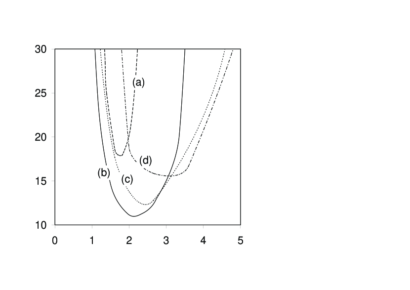
	$L/H$

Figure 1: The consumption power $P\cdot H$ (in kW.m) versus $L/H$ for different numbers of cells (a) $N_{c}=8$, (b) $N_{c}=18$, (c) $N_{c}=32$, (d) $N_{c}=50$.

In Figure 2, $P\cdot H$ is plotted versus $N_{c}$ for $L/H=2$ (full curve). We see that there is indeed a minimum around $N_{c}=20$ and that at large $N_{c}$, $P\cdot H$ increases with $N_{c}$ as predicted by (3). In a previous study Tilgner-97 , Tilgner calculated the critical magnetic Reynolds number for the Karlsruhe experiment geometry, varying the number of cells inside the device (Figure 4 of Tilgner-97 ). The resolution was made with a completely different method than the one used in Plunian-02a and it is then of interest to reconsider the results of Tilgner-97 in terms of power consumption and see how they compare to our results. For that we need to make preliminary correspondance between our present notations and those used in Tilgner-97 . In Tilgner-97 the flow container is a cylinder. then the consumption power, instead of (1), writes in the form $P\cdot H=\frac{\rho\eta^{3}}{\pi}\left(\frac{H}{R}\right)^{2}N_{c}^{2}R_{m}^{3}$ where $R$ is the cylinder radius. In Tilgner-97 we have $l=\frac{8}{4.1}\frac{R}{N_{T97}}$ where we call here $N_{T97}$ the parameter $N$ of Tilgner-97 . This leads to a number of cells $N_{c}=\frac{\pi R^{2}}{l^{2}}=0.825N_{T97}^{2}$. Furthermore the magnetic Reynolds number in Tilgner-97 is defined by $R_{mT97}=Ur_{0}/\eta$ where $r_{0}=\sqrt{1.25}R$ is the radius of the conducting sphere in which the cylinder is embedded. This leads to $R_{m}=\frac{1.745}{N_{T97}}R_{mT97}$. Finally using the results from the Figure 4 of Tilgner-97 , the consumption power is plotted versus the cells number on Figure 2 (dashed curve).

$P\cdot H$
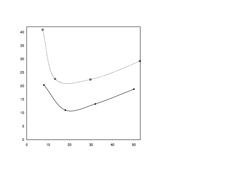
	$N_{c}$

Figure 2: The consumption power $P\cdot H$ (in kW.m) versus the cells number $N_{c}$. The full (dotted) curve is derived from Plunian-02a (from Tilgner-97 ) for $L/H=2$ ($R/H=1$).

We find that there is again an optimal scale separation for which the dissipated power is minimum and again it corresponds to $N_{c}$ close to 20. Furthermore the levels of power are of the same order of magnitude. We could not expect better agreement as the geometries and boundary conditions of Plunian-02a and Tilgner-97 are really different. Now considering the design of the Karlsruhe experiment, most of the dissipation power occurs in the pieces of pipes which redirect the flow into neighbouring cells at the end of each cell. The dissipation scaling in there is somewhat slower than $U^{3}$ but, most importantly, it is not proportional to the volume of the experiment. Therefore the scale separation of that experiment was guided by the characteristics of the available pumps Busse-96 in order to minimize the critical $R_{m}$, instead of minimizing the dissipated power, leading to $N_{c}=52$ (or alternatively to $N_{T97}=8$ corresponding to the minimum critical $R_{m}$ in Tilgner-97 ). Therefore the criterion that we derived here is relevant for propeller driven experiments, but the requirements are more complicated (and also less universal) for pump driven experiments.

- (1) R. Stieglitz and U. Müller, “Experimental demonstration of the homogeneous two-scale dynamo”, Phys. Fluids 13 3, 561-564 (2001)
- (2) G.O. Roberts, “Dynamo action of fluid motions with two-dimensional periodicity”, Phil. Trans. Roy. Soc. London A 271, 411-454 (1972)
- (3) F. Plunian and K.–H. Rädler, “Subharmonic dynamo action in the Roberts flow”, Geophys. Astrophys. Fluid Dynamics 96 2, 115-133 (2002)
- (4) S. Fauve and F. Pétrélis, “Effect of turbulence on the onset and saturation of fluid dynamos”, in Peyresq lectures on nonlinear phenomena, edited by J. Sepulchre, World Scientific, 1-64 (2003)
- (5) A. Tilgner, “A kinematic dynamo with a small scale velocity field”, Phys. Lett. A 226, 75-79 (1997)
- (6) F.H. Busse, U. Müller, R. Stieglitz and A. Tilgner, “ A two scale homogeneous dynamo: An extended analytical model and an experimental demonstration under development”, Magnetohydrodynamics 32, 259-271 (1996)