Viscoelastic subdiffusion: from anomalous to normal

Abstract

We study viscoelastic subdiffusion in bistable and periodic potentials within the Generalized Langevin Equation approach. Our results justify the (ultra)slow fluctuating rate view of the corresponding bistable non-Markovian dynamics which displays bursting and anti-correlation of the residence times in two potential wells. The transition kinetics is asymptotically stretched-exponential when the potential barrier $V_{0}$ several times exceeds thermal energy $k_{B}T$ ($V_{0}\sim 2\div 10\;k_{B}T$) and it cannot be described by the non-Markovian rate theory (NMRT). The well-known NMRT result approximates, however, ever better with the increasing barrier height, the most probable logarithm of the residence times. Moreover, the rate description is gradually restored when the barrier height exceeds a fuzzy borderline which depends on the power law exponent of free subdiffusion $\alpha$. Such a potential-free subdiffusion is ergodic. Surprisingly, in periodic potentials it is not sensitive to the barrier height in the long time asymptotic limit. However, the transient to this asymptotic regime is extremally slow and it does profoundly depend on the barrier height. The time-scale of such subdiffusion can exceed the mean residence time in a potential well, or in a finite spatial domain by many orders of magnitude. All these features are in sharp contrast with an alternative subdiffusion mechanism involving jumps among traps with the divergent mean residence time in these traps.

I Introduction

Multifaceted anomalous diffusion attracts ever increasing attention, especially in the context of biological applications. For example, diffusion of mRNAs and ribosomes in the cytoplasm of living cells is anomalously slow Golding , large proteins behave similarly Saxton ; Tolic ; Weiss1 ; Banks . Even intrinsic conformational dynamics of the protein macromolecules can be subdiffusive McCammon ; Bizzarri ; Kneller ; Luo ; Neusius ; Yang1 ; Granek ; Min1 ; Min2 ; Goychuk04 . There is a bunch of different physical mechanisms and the corresponding theories attempting to explain the observed behaviors, from spatial and/or time fractals, influence of disorder, cluster percolation, etc., to viscoelasticity of complex media Feder ; Hughes ; Scher ; Shlesinger ; Bouchaud ; Havlin ; Dewey ; Metzler ; Amblard ; Mason ; Qian ; Condamin ; Caspi . In particular, molecular crowding can be responsible for the viscoelasticity of dense suspensions like cytosol of bacterial cells lacking a static cytoskeleton Banks ; Mason ; Guidas . The state of the art remains rather perplexed, offering cardinally different views on the underlying physical mechanisms, as we clarify further with this work.

One physical picture reflects a set of the traps (possibly dynamical Condamin ) where the diffusing particle stays for a random time $\tau_{i}$. The mean residence time (MRT) in traps should diverge Scher ; Shlesinger for the diffusion to become anomalously slow, i.e. with the position variance growing sublinearly, $\langle\delta x^{2}(t)\rangle\sim t^{\alpha}$, with $0<\alpha<1$. This stochastic time-fractal picture became one of the paradigms in the field Hughes . It can be also related to averaging over static, or quenched disorder KlafterSilbey ; Hughes . Such a continuous time random walk (CTRW) among traps has infinite memory even if the residence times in the different traps are not correlated. The memory comes from the non-exponential residence time distributions in traps.

A quite different physical view was introduced by Mandelbrot et al. Mandelbrot ; Feder with the fractional Brownian motion (fBm). Here, the standard Gaussian Wiener process with independent increments is generalized to incorporate the statistical dependence of increments. The Gaussian nature remains untouched, but the increments can be either positively, or negatively correlated over an infinite range. Positive correlations (persistence) lead to superdiffusion. If correlations are anti-persistent, i.e. given a positive increment, the next one will, with greater probability, be a negative increment and vice versa, then a subdiffusive behavior can result. This idea does not imply that the residence time in a finite spatial domain diverges on average. Here roots the cardinal difference, in spite of some superficial similarities, between the fBm-based and the CTRW-based approaches to subdiffusion.

FBm emerges naturally, e.g., in viscoelastic media as one of the best justified models. Indeed, let us start from a phenomenological description of viscoelastic forces acting on a particle moving with velocity $\dot{x}(t)$ in some time-window $[0,t)$:

$$F_{v-el}(t)=-\int_{0}^{t}\eta(t-t^{\prime})\dot{x}(t^{\prime})dt^{\prime}.$$ (1)

Clearly, for a memory-less linear frictional kernel with $\eta(t)=2\eta\delta(t)$ on the particle acts a purely viscous Stokes friction force, $F_{v}=-\eta\dot{x}$. If memory does not decay, $\eta(t)=\eta=const$, then the force is quasi-elastic, $F_{el}(t)=-\eta[x(t)-x(0)]$ (cage force). A popular model of viscoelasticity introduced by Gemant Gemant , which interpolates between these two extremes, corresponds to $\eta(t)=\eta_{\alpha}t^{-\alpha}/\Gamma(1-\alpha)$ with $0<\alpha<1$ ($\Gamma(x)$ is the gamma-function). Remarkably, this model yields the Cole-Cole dielectric response for particles trapped in parabolic potentials Cole ; GoychukRapid , which is frequently observed in complex media. For a small Brownian particle of mass $m$, one must take into account unbiased random forces $\xi(t)$ acting from the environment (Langevin approach). Then, the linear friction approximation combined with the symmetry of detailed balance fixes the statistics of the stationary thermal random forces to be Gaussian Reimann . Moreover, the fluctuation-dissipation theorem dictates that the stationary autocorrelation function of the random force, temperature $T$, and the memory kernel are related Kubo :

$$\langle\xi(t)\xi(t^{\prime})\rangle=k_{B}T\eta(|t-t^{\prime}|)\;.$$ (2)

For Gemant model, $\xi(t)$ is the fractional Gaussian noise (fGn) Mandelbrot ; Min1 ; GoychukRapid . Altogether, the motion in potential $V(x,t)$ is described by the generalized Langevin equation (GLE)

$$m\ddot{x}+\int_{0}^{t}\eta(t-t^{\prime})\dot{x}(t^{\prime})dt^{\prime}+\frac{\partial V(x,t)}{\partial x}=\xi(t)\;.$$ (3)

Importantly, this GLE can also be derived from the mechanical equations of motion for a particle interacting with a thermal bath of harmonic oscillators, i.e. from first principles. This statistical-mechanical derivation Bogolyubov ; Kubo ; Zwanzig ; WeissBook involves the spectral density $J(\omega)$ of bath oscillators. It is related to the spectral density of thermal force, $S(\omega)=2\int_{0}^{\infty}\langle\xi(t)\xi(0)\rangle\cos(\omega t)dt$, as $S(\omega)=2k_{B}TJ(\omega)/\omega$. With $J(\omega)=\eta_{\alpha}\omega^{\alpha}$, the so-called Ohmic case of $\alpha=1$ corresponds to viscous Stokes friction and normal diffusion. The sub-Ohmic, or fracton thermal bath WeissBook ; Granek with $0<\alpha<1$ and $1/f^{1-\alpha}$ noise spectrum of random force corresponds to the above Gemant model of viscoelasticity. It yields subdiffusion in the potential-free case Wang ; WeissBook . The velocity autocorrelation function is then negative (except of origin), being the reason for the anti-persistent motion. The physical origin of this feature is that the elastic component of the viscoelastic force opposes the motion and ever tries to restore the current particle’s position. Moreover, in the inertialess limit ($m\to 0$) the solution of GLE is fBm with the coordinate variance $\langle\delta x^{2}(t)\rangle=2K_{\alpha}t^{\alpha}/\Gamma(1+\alpha)$ Caspi ; PRL07 and the subdiffusion coefficient $K_{\alpha}$ obeying the generalized Einstein relation $K_{\alpha}=k_{B}T/\eta_{\alpha}$ Chen ; MetzlerPRL . This way, anti-persistent subdiffusive fBm emerges from first principles within a physically well grounded, but approximate description. It corresponds also exactly to the diffusion equation with a time-dependent diffusion coefficient $D(t)=K_{\alpha}/[\Gamma(1+\alpha)t^{1-\alpha}]$ Adelman which is frequently used to fit experiments in viscoelastic and crowded environments, see e.g. in Saxton ; Banks ; Guidas .

II Theory

Anomalous escape (rate) processes and spatial subdiffusion in periodic potentials represent within the GLE description a highly nontrivial, longstanding challenge. Even the corresponding non-Markovian Fokker-Planck description is generally not available, except for the strictly linear and parabolic potentials Adelman . To get insight into the physics of such processes, it is convenient to approximate $1/f^{1-\alpha}$ noise by a sum of independent Ornstein-Uhlenbeck noise components, $\xi(t)=\sum_{i=0}^{N-1}\zeta_{i}(t)$, with the autocorrelation functions, $\langle\zeta_{i}(t)\zeta_{j}(t^{\prime})\rangle=k_{B}T\eta_{i}\delta_{ij}\exp(-\nu_{i}|t-t^{\prime}|)$. The corresponding memory kernel is accordingly approximated by a sum of exponentials,

$$\eta(t)=\sum_{i=0}^{N-1}\eta_{i}\exp(-\nu_{i}t),$$ (4)

where $\nu_{i}=\nu_{0}/b^{i}$ is the inverse autocorrelation time of the $i$-th component and $\eta_{i}=(\eta_{\alpha}/\Gamma(1-\alpha))C_{\alpha}(b)\nu_{0}^{\alpha}/b^{i\alpha}$ is its weight. Furthermore, $\nu_{0}$ presents the high-frequency cutoff of $\xi(t)$, $b$ is a dilation (scaling) parameter, and $C_{\alpha}(b)$ is a numerical constant. The low-frequency noise cutoff is $\omega_{c}=\nu_{0}/b^{N-1}$. It is worth to mention that such cutoffs emerge for any $1/f$ noise on the physical grounds Weissman . For $\alpha=0.5$, which is of experimental interest Min1 ; Min2 , the choice of $b=2$ (i.e. octave scaling) and $N=64$ with $\nu_{0}=10^{3}$ (in arbitrary units) and $C_{1/2}(2)=0.389$ allows one to fit perfectly the power law kernel in the range from $t=10^{-3}$ till $t=10^{15}$, i.e. over 18 time decades. The choice of $b=10$ (i.e. decade scaling) with $C_{1/2}(10)=1.3$ provides also an excellent fit over 15 time decades from $t=10^{-3}$ till $t=10^{12}$ with $N=16$. The numerical advantage of larger $b$ is that one can use smaller Markovian embedding dimension $D=N+2$. These two approximations to the exact power law memory are shown in Fig. 1. The approximation with $b=10$ displays logarithmic oscillations Hughes which are barely seen in this plot and make a little influence on the stochastic dynamics, see in Fig. 2.

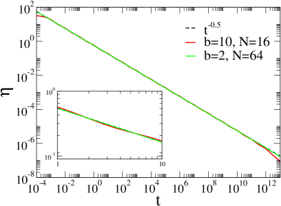
Figure 1: (Color online) Frictional power law memory kernel (in units of $\eta_{\alpha}$) and its two different approximations versus time $t$ (arbitrary units) for $\alpha=0.5$ and $\nu_{0}=10^{3}$. Notice that the approximation with $b=2$ practically coincides with the exact kernel in this plot and the choice $b=10$ is also a very good one in spite of logarithmic oscillations which are barely seen. Inset magnifies a part of plot.

Free subdiffusion holds until the time scale of $1/\omega_{c}$ which can be very large. The idea of such a representation of a power law dependence is rather old Palmer ; Hughes , being also habitual in the $1/f$ noise theory Weissman . The corresponding power spectrum is approximated by a sum of Lorentzians, $S(\omega)=2k_{B}T\sum_{i}\frac{\eta_{i}\nu_{i}}{\omega^{2}+\nu_{i}^{2}}$. Every stationary noise component is asymptotic ($t\to\infty$) solution of $\dot{\zeta}_{i}(t)=-\nu_{i}\zeta_{i}(t)+\sqrt{2\eta_{i}\nu_{i}k_{B}T}\xi_{i}(t)$, where $\xi_{i}(t)$ are independent white Gaussian noises with unit intensity, $\langle\xi_{i}(t)\xi_{j}(t^{\prime})\rangle=\delta_{ij}\delta(t-t^{\prime})$. Furthermore, the particle must act back on the source of noise in order to have the FDT relation (2) satisfied. This yields the following $D=N+2$ dimensional Markovian embedding of the non-Markovian GLE stochastic dynamics in Eq. (3) with kernel (4):

$$\dot{x} = v\;,$$ (5)

$$m\dot{v} = -\frac{\partial V(x,t)}{\partial x}+\sum_{i=0}^{N-1}u_{i}(t)\;,$$ (6)

$$\dot{u}_{i} = -\eta_{i}v-\nu_{i}u_{i}+\sqrt{2\nu_{i}\eta_{i}k_{B}T}\xi_{i}(t)\;.$$ (7)

Initial $u_{i}(0)$ have to be sampled independently from unbiased Gaussian distributions with the standard deviations $\sigma_{i}=\sqrt{k_{B}T\eta_{i}}$ Kupferman . Under this condition, it is easy to show that Eqs. (5)-(7) are equivalent to the GLE (3) with kernel (4) under FDT relation (2). Notice that $u_{i}(t)$ are auxiliary mathematical variables and should not be interpreted as (scaled) coordinates of some physical particles. The embedding (5)-(7) can be also derived from a more general scheme in Ref. Kupferman .

The numerical simulations of Markovian dynamics in Eqs. (5)-(7) below were done with stochastic Euler and Heun algorithms Gard using different random number generators. The results are robust. The simulations have been checked against the exact analytical results available for the potential-free case and parabolic potentials. The both above embeddings with $b=2,N=16$ and $b=10,N=64$ yield practically the same results within statistical errors. However, the simulations with $N=16$ requires much less computational time. Therefore, we preferred the latter $D=18$-dimensional embedding in most simulations following a “rule of thumb” Sansom : a negative power law extending over $n$ time-decades can be approximated by a sum of about $n$ exponentials. The quality of this approximation along with numerical errors is discussed in the Appendix A and Fig. 2 by making comparison of the numerical Monte Carlo results with the numerically exact solution of the free subdiffusion problem. The numerical error is mostly less than 3% for free subdiffusion in this work, whereas the theoretical error incurred by the $16$-exponential approximation of the power law memory kernel is mostly less than 1%, cf. Fig. 2. Clearly, it makes no sense to approximate the kernel better, if no more than $n=10^{4}$ trajectories are used in the ensemble averaging.

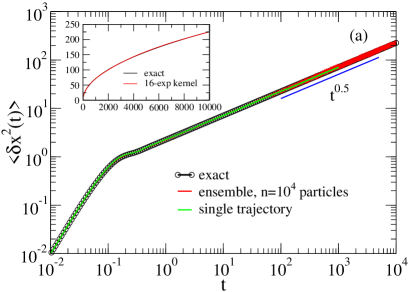
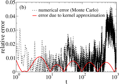
Figure 2: (Color online) (a) Stochastic simulations of Eqs. (5)-(7) with embedding dimension $D=18$ vs. exact solution of GLE (3) for free subdiffusion. Coordinate is scaled in some arbitrary units $L$ and time is scaled in units of $\tau_{\beta}=(L^{2}\eta_{\alpha}/k_{B}T)^{1/\alpha}$; $\alpha=0.5$ and the damping parameter $r_{\beta}=\tau_{\beta}/\tau_{\rm bal}=10$ with $\tau_{\rm bal}=L/v_{T}$ and $v_{T}=\sqrt{k_{B}T/m}$. Particles are initially localized at $x=0$ with Maxwellian distributed velocities. The number of particles $n=10^{4}$ is used in simulations (stochastic Heun algorithm, time step $\Delta t=10^{-4}$) for the ensemble averaging. The time averaging for a single trajectory is done using Eq. (19). The agreement proves ergodicity. Inset in compares two numerically exact solutions of GLE, one with the strict power law kernel and one with its $16$-exponential approximation. (b) Relative numerical error of our simulations (versus the exact solution) is presented. The relative deviation of the solution with the approximate memory kernel from the solution with exact power law kernel is also presented. Notice the occurrence of logarithmic oscillations within a less than 1% error margin, which, however, do not play any essential role.

The chosen Markovian embedding of non-Markovian GLE dynamics with $\eta(t)$ in Eq. (4) is mathematically, of course, not unique. Another embedding was proposed in Ref. Marchesoni and infinitely many different embeddings of one and the same non-Markovian dynamics are in fact possible Kupferman . However, our simplest scheme allows to contemplate straightforwardly the view of anomalous escape processes as rate processes with dynamical disorder Min2 ; Zwanzig2 ; WangWolynes .

II.1 Non-Markovian rate theory and beyond

We consider now stochastic transitions in a paradigmatic bistable quartic potential $V(x)=V_{0}(1-x^{2}/x_{0}^{2})^{2}$ with minima located at $x_{\rm min}=\pm x_{0}$ and the barrier height $V_{0}$. The question is: Which is the statistical distribution of the residence times in two potential wells and the escape kinetics? This is a long-standing problem for a general memory friction. Since the effective friction is sufficiently strong (the memory friction integral diverges) one can tentatively use a prominent non-Markovian rate theory (NMRT) result GroteHynes ; HanggiMojtabai ; Pollak ; HTB90 which is a generalization of the celebrated Kramers rate expression Kramers . It assumes asymptotically an exponential kinetics for the survival probability in one well, $P(t)\sim\exp[-R(\mu)t]$, with the non-Markovian rate

$$R(\mu)=\kappa(\mu)\frac{\omega_{0}}{2\pi}\exp(-\beta V_{0}).$$ (8)

In Eq. (8), $\omega_{0}=\sqrt{V^{{}^{\prime\prime}}(x_{\rm min})/m}=\sqrt{8V_{0}/(mx_{0}^{2})}$ is the bottom attempt frequency, $\exp(-\beta V_{0})$ is the Arrhenius factor, $\beta=1/(k_{B}T)$ is the inverse temperature, and

$$\kappa(\mu)=\frac{\mu}{\omega_{b}}\leq 1$$ (9)

is the transmission coefficient. It invokes the effective barrier frequency $\mu$ given by the positive solution of equation

$$\mu^{2}+\mu\tilde{\eta}(\mu)/m=\omega_{b}^{2},$$ (10)

where $\tilde{\eta}(s)=\int_{0}^{\infty}\exp(-st)\eta(t)dt$ is the Laplace-transformed memory kernel, and $\omega_{b}=\sqrt{|V^{{}^{\prime\prime}}(0)|/m}=\omega_{0}/\sqrt{2}$ is the (imaginary) barrier top frequency in the absence of friction. We focus below on the case of sufficiently high barriers, where the Arrhenius factor is small, $\exp(-\beta V_{0})\ll 1$. Clearly, a good single-exponential kinetics with exponentially distributed residence times, $\psi(\tau)=-dP(\tau)/d\tau$, can only be valid for such potential barriers, even in the strictly Markovian case.

However, how high is high? Could asymptotically exponential kinetics be attained for the viscoelastic model considered at all? Very important is that the relaxation within the potential well is ultraslow and this fact seems to invalidate the non-Markovian rate description generally PRL07 . To understand this, let us neglect formally for a while the inertia effects, $m\to 0$. Then, the strict power law kernel corresponds (in parabolic approximation) to the relaxation law $\langle\delta x(t)\rangle=\delta x(0)E_{\alpha}[-(t/\tau_{r})^{\alpha}]$ with the anomalous relaxation constant $\tau_{r}=[\eta_{\alpha}x_{0}^{2}/(8V_{0})]^{1/\alpha}$, where $E_{\alpha}(x)=\sum_{n=0}^{\infty}x^{n}/\Gamma(1+\alpha n)$ is the Mittag-Leffler function Min1 ; PRL07 . Asymptotically, $\langle\delta x(t)\rangle\propto(t/\tau_{r})^{-\alpha}$, being initially a stretched exponential. Precisely the same relaxation law holds also for the CTRW subdiffusion in the parabolic well MetzlerPRL which (along with other similarities for the potential-free case) gave grounds to believe that these two subdiffusion scenarios are somehow related, or similar. From the fact of ultraslow relaxation, it is quite clear that there cannot be a rate description even for appreciably high potential barriers, until the relaxation time within a potential well becomes negligible as compared with a characteristic time of escape. It worth to mention here that the non-Markovian rate theory approach yields a finite rate always, even for the strict power-law kernel Chaudhury , $R_{0}=R(\omega_{r}^{(b)})=\omega_{r}^{(b)}\exp(-\beta V_{0})/(\sqrt{2}\pi)$, where $\omega_{r}^{(b)}=[4V_{0}/(\eta_{\alpha}x_{0}^{2})]^{1/\alpha}$ is solution of Eq. (10) for $m\to 0$.

This cannot be, however, always correct. Indeed, let us introduce ad hoc a variable small-frequency cutoff $\nu_{c}$ such that $\tilde{\eta}(s)$ becomes $\tilde{\eta}(s)=\eta_{\alpha}(s+\nu_{c})^{\alpha-1}$. Then, choosing self-consistently $\nu_{c}=R(\mu)$ in Eqs. (8)-(10) (for $m\to 0$) one can show that the corresponding $\mu$ becomes modified as $\mu\to\mu^{*}=\omega_{r}^{(b)}[1+\exp(-\beta V_{0})/(\sqrt{2}\pi)]^{1/\alpha-1}$. From this we conclude that the non-Markovian rate expression $R(\mu)$ is practically not affected by such a cutoff when $\exp(-\beta V_{0})\ll 1$. This does not mean, however, that all the slowly fluctuating noise contributions with $\nu_{i}<R_{0}$ can be simply neglected. They lead, in fact, to the fluctuating rate description invalidating thereby the non-Markovian rate picture.

II.2 Fluctuating rates: simplest approximation

The idea is to divide all the noise components $\zeta_{i}$ into the two groups, $\xi(t)=\xi_{f}(t)+\xi_{s}(t)$: the fast noise $\xi_{f}(t)=\sum_{i\leq i_{c}}\zeta_{i}(t)$, which contributes to the “frozen” non-Markovian rate $R(\mu)$, and the slow modes which constitute the slowly fluctuating random force $\xi_{s}(t)=\sum_{i>i_{c}}\zeta_{i}(t)$. The separation frequency $\nu_{i_{c}}$ is chosen such that $\nu_{i}\leq\nu_{i_{c}}<R(\mu)$. It depends on the ratio of barrier height and temperature, as well as $\alpha$. Furthermore, let’s assume that for the slow $u_{i}$-modes in Eq. (7) one can approximately replace $v(t)$ by its average zero-value. This is a reasonable approximation because of the dynamics of $v(t)$ is fast on that time scale. Then, the corresponding equations for $u_{i}(t)$ decouple from the particle dynamics, $u_{i}\to\zeta_{i}$, and the corresponding stochastic modes can be considered just as an external random force. The fast noise agitates the particle trapped (otherwise) in the potential wells leading to the escape events. To a first approximation, one can regard the slow noise $\xi_{s}(t)$ be quasi-frozen on the time scale of such escape events. Then, for high barriers $\beta V_{0}\gg 1$ one can use a two-state approximation for the overall kinetics with the non-Markovian rate $R(\mu^{*},\xi_{s})$ slowly driven in time by $\xi_{s}(t)$. This slow stochastic force is in fact also power-law correlated. Thus, we are dealing with a typical problem of non-Markovian dynamical disorder Goychuk05 . Some insight can be obtained by using the quasi-static disorder approximation Austin ; Zwanzig2 ; Dewey ; Goychuk05 for the averaged kinetics,

$$P_{1,2}(t)=\int_{-\infty}^{\infty}w(\xi_{s})\exp[-R_{1,2}(\mu^{*},\xi_{s})t],$$ (11)

where $R_{1,2}(\mu^{*},\xi_{s})$ are the non-Markovian rates for a quasi-static biasing force $\xi_{s}$ distributed with the Gaussian probability density $w(\xi_{s})=1/(\sqrt{2\pi}\sigma_{s})\exp(-\xi_{s}^{2}/(2\sigma_{s}^{2}))$ and variance $\sigma_{s}^{2}=k_{B}T\eta_{s}$, where $\eta_{s}=\sum_{i>i_{c}}\eta_{i}$. The calculation of $\sigma_{s}$ for $\alpha=0.5$ (or larger) shows that the bias fluctuations are sufficiently small for $\beta V_{0}\geq 2$, so that the approximation $R_{1,2}(\mu^{*},\xi_{s})\approx R(\mu^{*})\exp[\pm\xi_{s}x_{0}/(k_{B}T)]$ can be used. Here, we just assume that the rms of potential barrier modulations $\pm\sigma_{s}x_{0}$ is small against $V_{0}$. Since the influence of slow modes on the effective barrier frequency $\mu$ is exponentially small for high barriers (see above), one can replace $R(\mu^{*})$ with $R(\mu)$. This finally yields

$$P_{1,2}(t)\approx\int_{0}^{\infty}\exp[-R(\mu)t\;y]W(y)dy,$$ (12)

where $W(y)=1/(\sqrt{2\pi}dy)\exp[-\ln^{2}(y)/(2d^{2})]$ is the probability density of log-normal distribution with width $d=\sqrt{\eta_{s}x_{0}^{2}/(k_{B}T)}$. The corresponding mean residence time (MRT) and the relative standard deviation, $\delta\sigma=\sqrt{\langle\tau^{2}\rangle-\langle\tau\rangle^{2}}/\langle\tau\rangle$, are:

$$\langle\tau\rangle=R^{-1}(\mu)\exp(d^{2}/2),$$ (13)

$$\delta\sigma=\sqrt{2\exp(d^{2})-1}=\sqrt{2[\langle\tau\rangle R(\mu)]^{2}-1}.$$ (14)

To characterize non-Markovian kinetics, one can introduce also a time-dependent rate $k(t)=-d\ln P(t)/dt$ which decays asymptotically to zero for any finite width $d$ within this approximation.

The resulting physical picture becomes clear: Fast Ornstein-Uhlenbeck components with $\nu_{i}>R(\mu)$ participate in forming the non-Markovian rate $R(\mu)$, while the slow ones lead to a stochastic modulation of this rate in time. This implies the following main features which are confirmed further by a numerical study: (i) Both the mean residence time in a potential well, and all the higher moments exist. (ii) Anti-correlations between the alternating residence time intervals in the potential wells emerge along with a profoundly bursting character of the trajectory recordings, cf. Fig. 3. Indeed, during the time of a quasi-frozen stochastic tilt many transitions occur between the potential wells. The shorter time in the (temporally) upper well is followed by a longer time in the lower well. This yields anti-correlations (cf. Fig.4). Moreover, many short-living transitions into the temporally upper well occur, which appears as bursting (cf. Fig. 3). The subsequent sojourns in one potential well are also positively correlated for many transitions (not shown). (iii) The escape kinetics is clearly non-exponential, see in Fig. 5 and below. (iv) The corresponding power spectrum of bistable fluctuations has a complex structure with several different $1/f$ noise low-frequency domains (cf. Fig. 6); (v) The higher is potential barrier, the smaller is the rms of slow rate fluctuations. The last circumstance implies that for very high barriers the exponential escape kinetics with non-Markovian rate in (8)-(10) will be restored, cf. Fig. 10. For small $\alpha$, this however can require very high barriers and be practically unreachable.

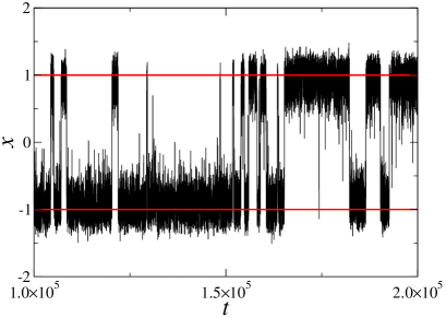
Figure 3: (Color online) A sample trajectory of bistable transitions for $\beta V_{0}=6$. Time is given in units of $\tau_{r}^{(b)}=[\eta_{\alpha}x_{0}^{2}/(4V_{0})]^{1/\alpha}$ and coordinate in units of $x_{0}$. The residence time distributions are extracted by using the two thresholds (red lines). Stochastic Heun algorithm with the time step $\Delta t=10^{-3}$ and Mersenne Twister pseudo-random number generator, combined with the Box-Muller algorithm are used. Markovian embedding with $N=16$ is used as described in the text. $\alpha=0.5$, $r=10$, $b=10$, $\nu_{0}=1000$.

II.3 Numerical results

Let us compare now these theoretical predictions with numerical results. The time is scaled in this section in the units of $\tau_{r}^{(b)}=1/\omega_{r}^{(b)}=[\eta_{\alpha}x_{0}^{2}/(4V_{0})]^{1/\alpha}$, which is the anomalous relaxation constant for the inverted parabolic barrier in the overdamped limit, and the role of inertial effects is characterized by the dimensionless parameter $r=\omega_{b}\tau_{r}^{(b)}$. The used $r=10$ corresponds to the overdamped limit in the case of normal diffusion. For the used $16$-exponential approximation of the memory kernel, it yields $\mu\approx 0.999$ in Eq. (10) which is very close to $\mu=1$ corresponding to the formal overdamped limit, $m\to 0$, with the transmission coefficient $\kappa=1/r=0.1$. Despite this fact, some inertia effects for the intra-well relaxation dynamics are still present. Generally, it is important to include such effects for a power law memory kernel Burov . We performed simulations of very long trajectories (from $5\cdot 10^{3}$ to $10^{6}$ transitions between wells) achieving statistically trustful results in each presented case. A sample of stochastic trajectory for $\beta V_{0}=6$ is shown in Fig.  3. The bursting character is clear Goychuk05 , indicating also slow tilt fluctuations.

To extract the residence time distributions (RTDs) in the wells, $\psi_{1}(\tau_{1})$ and $\psi_{2}(\tau_{2})$, and their joint distribution $\psi(\tau_{1},\tau_{2})$, two thresholds were set at the minima of the potential wells, cf. Fig. 3. Fig. 4 displays the the joint distribution $\psi(\ln(\tau_{1}),\ln(\tau_{2}))$ of the logarithmically transformed residence times for $\beta V_{0}=2$. Two facts are self-evident: (1) the transformed distribution is not sharply peaked and spreads over several time decades; (2) the subsequent residence times in two potential wells are significantly anti-correlated. The normalized covariance between $\tau_{1}$ and $\tau_{2}$ is $c(\tau_{1},\tau_{2})\approx-0.116$, and between the logarithmically transformed variables $c(\ln\tau_{1},\ln\tau_{2})\approx-0.19$. The mean residence time is approximately $\langle\tau_{1,2}\rangle\approx 52$ with the relative standard deviation $\delta\sigma_{1,2}=\sqrt{\langle\tau_{1,2}^{2}\rangle-\langle\tau_{1,2}\rangle^{2}}/\langle\tau_{1,2}\rangle\approx 1.69$, whereas the non-Markovian rate theory yields $\tau_{\rm NM}=1/R(\mu)\approx 32.9$. This value essentially underestimates MRT, but it lies not far away from the extended region of most probable $\ln\tau_{1,2}$(see the green symbol in Fig.  4). Furthermore, the distribution of the residence times in each potential well, $\psi(\tau)=-\dot{P}(\tau)$, is profoundly non-exponential, with a complex kinetics being mostly stretched-exponential, $P(\tau)\sim\exp[-(\tau/\tau_{\gamma})^{\gamma}]$. The power $\gamma$ slightly varies in time and reaches asymptotically $\gamma\approx 0.65$, as indicated by a straight line trend for $-\ln[P(\tau)]$ on the doubly-logarithmic plot in Fig. 5. Generally, the asymptotic value of $\gamma$ is bounded as $\alpha\leq\gamma<1$ and depends on the ratio $V_{0}/k_{B}T$. The formally defined time-dependent non-Markovian rate decays to zero as $k(t)\propto 1/t^{1-\gamma}$ and the corresponding power spectrum of fluctuations in Fig.  6 displays a complex $1/f^{\gamma}$-noise pattern with the same $\gamma\approx 0.65$ at lowest frequencies. Overally, the non-Markovian rate theory approach is clearly not applicable for such a barrier.

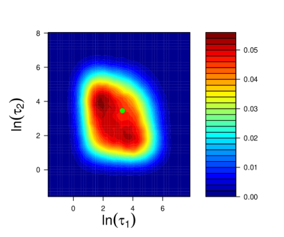
Figure 4: (Color online) Two-dimensional distribution of the log-transformed residence times in the potential wells for $\beta V_{0}=2$. The green symbol corresponds to the non-Markov rate theory result (for the studied $16$-exponential expansion of the power-law memory kernel). The orientation and the structure of the plateau of maximal probabilities manifest anti-correlation of the residence times in two potential wells. This feature is completely beyond the non-Markovian rate theory. Statistical software R R is used for data analysis and to produce the plot.

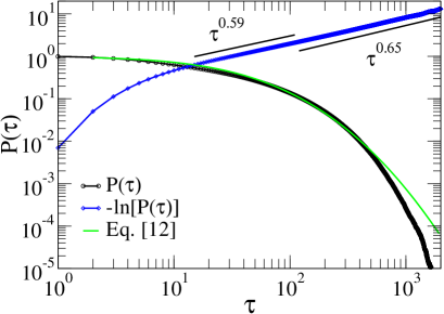
Figure 5: (Color online) Survival probability in one potential well versus time (in units of $\tau_{r}^{(b)}=[\eta_{\alpha}x_{0}^{2}/(4V_{0})]^{1/\alpha}$) for $\beta V_{0}=2$. The asymptote is stretched-exponential with $\gamma\approx 0.65$. Fit with Eq. (12) is done using $d=0.81$ and $R=2.67\cdot 10^{-2}$. These values were derived from the numerical data using the first two moments of the numerical distribution and Eqs. (13), (14).

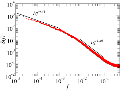
Figure 6: (Color online) The low-frequency part of the power spectrum of fluctuations for $\beta V_{0}=2$. The $1/f^{\gamma}$ feature for smallest frequencies is defined chiefly by the stretched-exponential asymptotics of the survival probability, cf. Fig. 3. The correlogram method along with the SSA-MTM Toolkit for Spectral Analysis Ghil is used to produce the spectrum.

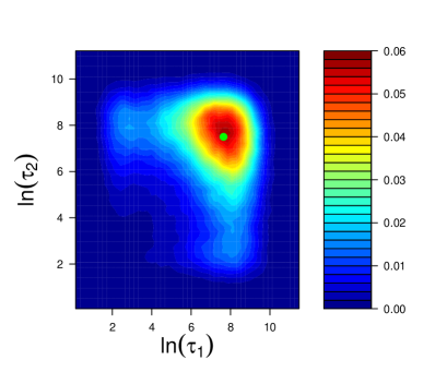
Figure 7: (Color online) Two-dimensional distribution of the log-transformed residence times in the potential wells for $\beta V_{0}=6$. The non-Markovian rate theory result (green symbol) yields the most probable value of $\ln(\tau_{1,2})$. Kinetics is, however, clearly non-exponential, even asymptotically.

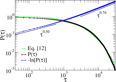
Figure 8: (Color online) Survival probability in one potential well versus time (in units of $\tau_{r}^{(b)}$) for $\beta V_{0}=6$. Asymptotics is stretched exponential with $\gamma\approx 0.76$. Initial kinetics is stretched exponential with $\gamma\approx\alpha$. Fit with Eq. (12) is done using $d=0.634$ and $R=4.48\cdot 10^{-4}$. These values were derived from the numerical data using the first two moments of the distribution and Eqs. (13), (14).

The qualitatively similar features remain also for some higher potential barriers (or lower temperatures), e.g. for $\beta V_{0}=6$. In this case, numerically $\langle\tau_{1,2}\rangle\approx 2710$, and $\delta\sigma_{1,2}\approx 1.41$, whereas the non-Markovian rate theory yields $\tau_{\rm NM}\approx 1794$ with $\ln(\tau_{\rm NM})\approx 7.49$. This NMRT result compares, however, now well against the most probable $\ln(\tau_{1,2})$ in Fig. 7. This provides one of important results: Even if the non-Markovian rate theory is still not applicable, it can predict remarkably well the most probable logarithm of residence times. The kinetics remains asymptotically stretched-exponential even for such a high barrier with $\gamma$ increased to $\gamma\approx 0.76$ (cf. Fig. 8). However, the region of most probable $\ln\tau_{1,2}$ shrinks further with increasing $\beta V_{0}$ and the non-Markovian rate theory describes ever better both the most probable $\ln\tau_{1,2}$, and the (logarithm of) mean residence time which start to merge as it should be for a single-exponential RTD. Already for $\beta V_{0}=10$ the whole distribution is well approximated by the stretched exponential with $\gamma\approx 0.90$, Fig. 9.

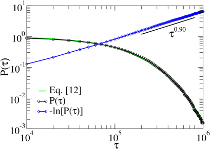
Figure 9: (Color online) Survival probability in one potential well versus time (in units of $\tau_{r}^{(b)}$) for $\beta V_{0}=10$. Using a fit to the survival probability, the whole distribution is well described by a stretched exponential with $\gamma\approx 0.90$. The maximum likelihood fit to the numerical data yields but a slightly different value $\gamma\approx 0.85$, cf. in Fig. 10, indicating that the whole distribution is not properly stretched exponential. It is rather described by Eq. (12) with $d=0.335$ and $R=8.26\cdot 10^{-6}$. These values were derived from the numerical data using the first two moments of the distribution and Eqs. (13), (14).

Clearly, for ever higher barriers the transition kinetics becomes gradually single-exponential. This happens when the barrier height exceeds some characteristic value $V_{c}(\alpha,T)$ which depends on $\alpha$ and temperature, cf. Fig. 10. Since there is no a precise threshold, the definition of $V_{c}$ is rather ambiguous. A working criterion for defining $V_{c}$ can be, e.g., that the rate description is achieved within some error bound, e.g. $1\%$ for deviation of $\gamma$ from unity.

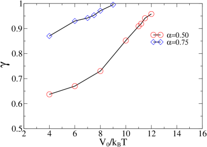
Figure 10: (Color online) Power exponent of a (single) stretched exponential fit to the overall residence time distribution versus the barrier height for two different subdiffusion exponents $\alpha$. The maximum likelihood approach is used to derive $\gamma$ from data. Notice that this $\gamma$ does not correspond to the asymptotic $\gamma$ in the previous figures and text, but rather presents an average of $\gamma(t)$ changing slowly in time. This subtle difference diminishes when $\gamma$ approaches one. For $\alpha=0.75$, $C_{0.75}=1.885$; other parameters in the kernel approximation are the same as for $\alpha=0.5$. For $V_{0}$ exceeding some borderline value $V_{c}(\alpha,T)$, $\gamma$ tends to one and kinetics becomes gradually single exponential.

For $\beta V\gg\beta V_{c}$, the overall escape kinetics is well-described by the non-Markovian rate theory. For $\alpha=0.5$ it is very difficult to obtain a good statistics of transitions to find precisely this borderline. For the maximal value $\beta V_{0}=12$ used in our simulations the maximum likelihood fit with a stretched exponential (Weibull) distribution yields $\gamma=0.952\pm 0.034$. This value of $\beta V=12$ provides an estimate for $\beta V_{c}$ from below for $\alpha=0.5$. It approximately delimits the borderline between the applicability of NMRT for $\alpha=0.5$ and our treatment beyond it. The lower is $\alpha$, the higher is borderline $\beta V_{c}(\alpha)$, and vice versa. For example, for $\alpha=0.75$, $\beta V_{c}$ reduces to about $\beta V_{c}\approx 9$. For these parameters, the maximum likelihood fit of the numerical data with the single exponential distribution yields the rate $R=(2.864\pm 0.065)\cdot 10^{-5}$ which only slightly deviates (about 3% of error) from the corresponding non-Markovian rate theory result $R(\mu)\approx 2.775\cdot 10^{-5}$. And for $\beta V_{0}=10$, the maximum likelihood fit yields $R=(1.056\pm 0.034)\cdot 10^{-5}$ ($\alpha=0.75$) which almost agree within statistical errors with the non-Markovian rate theory result $R(\mu)=1.021\cdot 10^{-5}$. This provides a spectacular confirmation of both the non-Markovian rate theory for very high potential barriers, and the reliability of our numerics, as well as the physical picture of anomalous escape developed in this work. On the contrary, for $\alpha<0.5$, e.g. $\alpha=0.25$, $\beta V_{c}$ can be so high that the non-Markovian rate theory limit will never be reached for realistic barrier heights. Both our theoretical argumentation and the numerical results show that this borderline is fuzzy and and the rate description is restored gradually. The tendency in Fig. 10 is, however, obvious.

The quasi-static disorder approximation cannot describe quantitatively the numerical results for a broad range of parameters (rate disorder is yet dynamical, in spite of a quasi-infinite autocorrelation time Goychuk05 ). Nevertheless, it captures the essential physics (cf. Figs. 5,8) and becomes ever better with increasing the barrier height, cf. Fig. 9. The agreement in this figure proves that our theory is essentially correct predicting the correct trend with increasing the barrier height, at least for $\alpha>0.5$. Indeed, with increasing the barrier height, or lowering the temperature the averaged escape time increases exponentially with $\beta V_{0}$ and, therefore, ever more slow noise components $\zeta_{i}$ contributes to the non-Markovian rate and ever less such components contributes to fluctuation of this rate. For this reason, the root mean-squared amplitude of the slow (in our terminology) stochastic force $\xi_{s}(t)$ gradually diminishes. For some characteristic $\beta V_{c}$, which clearly depends on $\alpha$, it becomes negligible and the single-exponential kinetics is then approximately restored. The corresponding rate is given by the non-Markovian rate theory.

The physical picture developed in this work is very different from the previous attempts in Refs. Chaudhury ; PRL07 to solve the problem of anomalous escape utilizing different approximations. The Ref. Chaudhury focuses on the subdiffusive transmission through the parabolic barrier. It predicts that asymptotic rate $k_{\infty}=-\lim_{t\to\infty}d\ln P(t)/dt$ always exists and is given precisely by the non-Markovian rate theory result in Eqs. (8)-(10). This is clearly not correct for $V<V_{c}(\alpha,T)$. Strictly speaking, $k_{\infty}=0$ always, even for $V>V_{c}(\alpha,T)$ for a strictly power law memory kernel. However, for $V\gg V_{c}(\alpha,T)$, the shape factor of Weibull distribution $\gamma$ equals approximately one, $\gamma\approx 1$, and the rate description provides a good approximation. The higher is $V_{0}$, the better is this approximation, cf. Fig. 10. The Ref. PRL07 focuses on the escape of a massless particle ($m\to 0$) from a parabolic potential well with a sharp cusp-like cutoff, utilizing the non-Markovian Fokker-Planck equation (NMFPE) of Refs. Adelman ; GroteHynes ; HanggiMojtabai . This NMFPE is exact for the parabolic potential, being but only approximate for a parabolic potential with cutoff. The better is the Gaussian approximation, the better should be the corresponding description, which implies high potential barriers $\beta V_{0}\gg 1$. The theory in PRL07 cannot be compared directly with the present one (different potentials, zero mass particle in PRL07 , expansion of the power law kernel into a finite sum of exponentials here), and the extrapolation of some main results in Ref. PRL07 on a more realistic case here, would lead to the conclusions which are at odds with the present theory. In particular, the theory in PRL07 predicts (for a strict power law kernel, without inertial effects) that the escape kinetics is asymptotically a power law, being only initially stretched exponential, and that the corresponding effective power law exponent tends exponentially to zero with increasing $\beta V_{0}$. This means that the particle becomes strongly localized with increasing the barrier height, and the corresponding kinetics becomes ever more abnormal. On the contrary, the present theory predicts that the escape kinetics tends to a normal one, even if it decelerates dramatically. For a memory kernel with cutoff, the theory in Ref. PRL07 predicts that with increasing the barrier height the kinetics does become normal, when the memory cutoff becomes shorter than the mean escape time. This prediction concords with the present theory. The difference is however that the physical picture developed in this work suggests that the escape kinetics can be also approximately exponential when the memory cutoff largely exceeds the mean escape time. To conclude, the theory in this work is more physical. It overcomes the previous attempts to solve the very nontrivial problem of subdiffusive escape by taking a quite different road of multidimensional Markovian embedding and it is confirmed by numerics.

The fact that the escape kinetics tends to a single-exponential with increasing the barrier height does not mean, however, that the diffusion becomes normal in the periodic potentials, as one might naively think in analogy with the CTRW theory. As a matter of fact, asymptotically such a diffusion cannot be faster that one in the absence of potential, i.e. $\langle\delta x^{2}(t)\rangle\propto t^{\alpha}$. Therefore, we expect here new surprises.

III Subdiffusion in periodic potentials

We consider a common type washboard potential $V(x)=-V_{0}\cos(2\pi x/L)$ with the spatial period $L$. To study the influence of periodic potential on free subdiffusion, it is convenient to scale now the time in the units of $\tau_{\beta}=(\beta L^{2}\eta_{\alpha})^{1/\alpha}$, as in Fig. 2, which does not depend on the barrier height $2V_{0}$. It takes time about $\tau_{\beta}$ to subdiffuse freely over the distance about $L$. Indeed, the numerical simulations for $\beta V_{0}=2$ delivers a surprise indicating, see in Fig.  11, that the presence of periodic potential does not influence subdiffusion asymptotically. This seems to agree with a theory in Refs. Chen ; WeissBook which, however, cannot be invoked directly because of it relates to a fully quantum case, where the tunneling effects generally contribute. From this agreement we can, however, conclude that this surprising effect is certainly not of the quantum nature in the quantum case, but reflects the anti-persistent character of our viscoelastic subdiffusion which is purely classical. Namely, it is not diverging MRT, but extremally long-lived displacement (and velocity) anti-correlations which are responsible for the observed anomalous diffusion behavior in viscoelastic media. It must be emphasized, however, this asymptotical regime is achieved through very long transients with a time-dependent $\alpha_{\rm eff}(t)$ gradually approaching $\alpha$, cf. Fig.  11. This feature is totally beyond any asymptotical analysis like one in Ref. Chen . The potential barrier height does generally matter and it strongly influences the whole time-course of diffusion. After a short ballistic stage followed by decaying coherent oscillations due to a combination of inertial and cage effects Burov in a potential, the diffusion can look initially close to normal (as for $\beta V_{0}=4$ in Fig.  11). This is due to a finite mean residence time in a potential well. However, it slows down and turns over into subdiffusion. The borderline of free subdiffusion cannot be crossed, cf. Fig. 11.

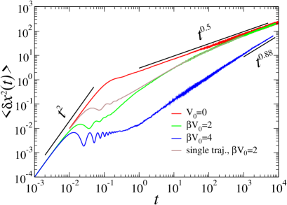
Figure 11: (Color online) Diffusion in washboard potentials. The distance is measured in units of period $L$ and the time in units of $\tau_{\beta}=(\beta L^{2}\eta_{\alpha})^{1/\alpha}$. $\alpha=0.5$ and the damping parameter $r_{\beta}=\tau_{\beta}/\tau_{\rm bal}=10$ with $\tau_{\rm bal}=L/v_{T}$ and $v_{T}=\sqrt{k_{B}T/m}$. Particles are initially localized at $x=0$ with Maxwellian distributed velocities. The number of particles $n=10^{4}$ is used in simulations (stochastic Heun algorithm, time step $\Delta t=10^{-4}$) for the ensemble averaging. Initially, the diffusional broadening is always ballistic due to inertia effects. In potentials, this regime is followed by transient rattling oscillations due to a combination of the cage effect and the influence of the potential force. On the space scale $\delta x>L$, diffusion becomes ultraslow $\langle\delta x^{2}(t)\rangle\propto t^{\alpha_{\rm eff}(t)}$ with a slowly changing $\alpha_{\rm eff}(t)$ which depends on the potential height. Asymptotically, $\alpha_{eff}(t\to\infty)\to 0.5$. This universal asymptotics is almost reached for $\beta V_{0}=2$.

Very important is that the free viscoelastic subdiffusion is ergodic, in agreement with Deng . The results of the ensemble averaging with $n=10^{4}$ particles coincide with the time averaging for a single particle done in accordance with Eq. (19), see in Fig. 2(a). However, in the periodic potential a strong deviation from the ergodic behavior takes place on the averaged time scale of the escape to the first neighboring potential wells, cf. Fig. 11. This reflects anomalous escape kinetics as discussed above. Nevertheless, on a larger time-scale the single-trajectory averaging and the ensemble averaging yield again the same results. All this is in striking contrast with the CTRW-based subdiffusion, both free Hughes ; Shlesinger ; He ; Lubelski and in periodic potentials Rapid06 ; Heinsalu06 . In this respect, the benefit which subdiffusional search can bring for functioning the biological cells machinery Golding ; Guidas will not be questioned by the weak ergodicity breaking, as it might be in the case of CTRW-based subdiffusion. Indeed, the weak ergodicity breaking is related to a spontaneous localization of CTRW-subdiffusing particles – i.e., a portion of them does not move at all (individual diffusion coefficient is close to zero), while other diffuse with an inhomogeneously distributed normal diffusion coefficient He ; Lubelski which depends on the total observation time ${\cal T}$, even if the particles are totally identical. Numerically, or in a real experimental setup the ergodic behavior is achieved in the case of viscoelastic subdiffusion for very long ${\cal T}$ only, see also in Deng . So, to check the ergodicity for times until $t=10^{3}$ we run a single trajectory for overall ${\cal T}=10^{7}$ (this corresponds roughly to sampling over $n=10^{4}$ copies, in analogy with the ensemble averaging). For a much smaller ${\cal T}$, the difference between the time and ensemble averagings becomes sizeable. Hence, experimentally one can yet observe broadly distributed subdiffusion coefficients, especially if both the particles and their environments are subjected to statistical variations Golding . However, differently from the CTRW subdiffusion, a particle will never get spontaneously trapped for the time of observation. This provides a true benchmark to distinguish between these two very different subdiffusion mechanisms experimentally.

IV Summary

Our main results are of profound importance for the anomalous diffusion and rate theory settling a long-standing and controversial issue with conflicting results of different approaches, and different approximations. In particular, we prove that subdiffusion does not require principally a divergent mean residence time in a finite spatial domain, which makes it less anomalous when the anti-persistent, viscoelastic mechanism is at work. Moreover, we substantiate the validity of the celebrated non-Markovian rate theory result (8)-(10) for very high potential barriers ($\beta V_{0}>12$ for $\alpha=0.5$ and $\beta V_{0}>\beta V_{c}\approx 9$ for $\alpha=0.75$ ) even for a strict power law memory kernel, where it was not expected to work because of an ultraslow relaxation within a potential well. However, for small $\alpha<0.5$ the corresponding borderline value $\beta V_{c}(\alpha)$ can be so high that this regime becomes practically unreachable, at least for numerical simulations. Surprisingly, the non-Markovian theory result remains useful also for intermediate barriers, $2k_{B}T<V_{0}<V_{c}(\alpha,T)$, where it predicts the most probable logarithm of dwelling times. Here, the physics is well described by slowly fluctuating non-Markovian rates. For small barriers, $\beta V_{0}<1$, and for other models, e.g. when the bottom of potential well becomes more extended and flat, like the potential box in PNAS02 , the fluctuating rate approach also loses its heuristic power. Then, the sluggish approach from the bottom to the barrier crossing region determines the transition kinetics. Even in the case of normal diffusion, different power-law kinetic regimes emerge PNAS02 and the anomalous intrawell diffusion can change the corresponding power-law exponents, as modeled within the CTRW approach in Ref. Goychuk04 .

One of generic results is that the CTRW subdiffusion and the GLE subdiffusion are profoundly different, in spite of some superficial similarities. Subdiffusion in periodic potentials highlights the differences especially clear. Surprising is the finding that asymptotically the GLE subdiffusion is not sensitive to the barrier height, even if imposing a periodic potential does strongly affect the overall time-course of diffusion, and for a high potential barrier subdiffusion can look normal on a pretty long time interval. However, it slows down and asymptotically approaches the borderline of free subdiffusion. Such subdiffusion operates within a quite different (as compared with CTRW) physical mechanism based on the anti-persistent long-range correlations and not on the residence time distributions with divergent mean.

We believe that our results require to look anew on the theoretical interpretation of experimental subdiffusion results in biological applications, where the issue of ergodicity can be crucial. They provide some additional theoretical support for the viscoelastic subdiffusion mechanism. A further detailed study is, however, necessary. To conclude, our work consolidates viscoelastic subdiffusion and fractional Brownian motion with the non-Markovian rate theory and fluctuating rate (dynamical disorder) approaches. It also agrees with the already textbook view [see, e.g. in Nelson (pp. 380-382)], of the unusual kinetics as one with quasi-frozen and quasi-continuous conformational substates, as it was pioneered in biophysical applications by Austin et al.Austin .

Appendix A Exact solution of the potential-free problem versus Monte Carlo simulations

In this Appendix, we discuss numerical errors by comparison of the approximate results with the exact solution of subdiffusion problem in the absence of any potential. This exact solution is well-known Wang ; Kupferman . Assuming initial velocities to be thermally distributed, it reads

$$\langle\delta x^{2}(t)\rangle=2v_{T}^{2}\int_{0}^{t}H(t^{\prime})dt^{\prime},$$ (15)

where

$$H(t)=\int_{0}^{t}K_{v}(\tau)d\tau$$ (16)

is the integral of normalized equilibrium velocity autocorrelation function $K_{v}(\tau):=\langle v(t+\tau)v(t)\rangle/\langle v^{2}(0)\rangle$ with $\langle v^{2}(0)\rangle=v_{T}^{2}=k_{B}T/m$. It has the Laplace-transform

$$\tilde{K}_{v}(s)=\frac{1}{s+\tilde{\eta}(s)/m}\;.$$ (17)

Accordingly, the Laplace-transform of the coordinate variance$,\langle\delta\tilde{x^{2}}(s)\rangle:=\int_{0}^{\infty}\exp(-st)\langle\delta x^{2}(t)\rangle dt$, is

$$\langle\delta\tilde{x}^{2}(s)\rangle=\frac{2v_{T}^{2}}{s^{2}[s+\tilde{\eta}(s)/m]}\;,$$ (18)

For the strict power-law kernel, Eq. (18) becomes $\langle\delta\tilde{x}^{2}(s)=2/[s^{3}/r^{2}+s^{1+\alpha}]$ with the distance measured in some arbitrary units $L$ and time in the units of $\tau_{\beta}=(L^{2}\eta_{\alpha}/k_{B}T)^{1/\alpha}$. This result can be inverted to the time domain in terms of the generalized Mittag-Leffler functions, see e.g. in Burov . However, both for the exact memory kernel and for its approximation in Eq. (4), it is convenient to invert Eq. (18) numerically using the Gaver-Stehfest method Stehfest with arbitrary numerical precision, as done e.g. in Ref. GoychukChemPhys for a different problem. The results thus obtained are numerically exact and the algorithm is very fast. They are compared against the results of the Monte-Carlo simulation of Eqs. (5)-(7) in Fig. 2. In these simulations, we used both the ensemble averaging over $n=10^{4}$ trajectories and a time averaging for single trajectory defined by

$$\langle\delta x^{2}(t)\rangle_{\cal T}=\frac{1}{{\cal T}-t}\int_{0}^{{\cal T}-t}[x(t+t^{\prime})-x(t^{\prime})]^{2}dt^{\prime}\,$$ (19)

for a very large time window ${\cal T}\gg t$. The relative error in Fig. 2(b) is calculated as $\delta=|\langle\delta x^{2}_{\rm exact}(t)\rangle-\langle\delta x^{2}_{\rm approx}(t)\rangle|/\langle\delta x^{2}_{\rm exact}(t)\rangle$, where $\langle\delta x^{2}_{\rm approx}(t)\rangle$ is either the result of numerical solution of stochastic differential equations (Monte Carlo, with $10^{4}$ trajectories – noisy looking data), or the result of $16$-exponential approximation in Eq. (18). The agreement is confirming both for the used approximation of the memory kernel and for the quality of our stochastic simulations. The error introduced by the kernel approximation is mostly less than 1%. The well-known phenomenon of logarithmic oscillations Hughes occurs within this error margin, and, therefore, practically does not influence our stochastic numerics, which have a typical error of less than 3% (maximal 5%). Notice that some damped oscillations in Fig.11 are of the inertial origin and have nothing in common with the logarithmic oscillations seen in Fig. 2(b). Moreover, for the octave scaling, $b=2$, and for $N=64$ such logarithmic oscillations are even not present in the variance behavior (not shown). The error margin in the variance behavior did not become, however, appreciably narrower. Therefore, such logarithmical oscillations practically do not matter for our numerics and the used $N=16$ embedding computationally is even preferred.

It worth to mention that the final time $t=10^{4}$ in our simulations with $n=10^{4}$ trajectories corresponds to about one week of computational time. Therefore, on our computers the theoretical limit of free normal diffusion for $t>10^{12}$ for the used $N=16$ embedding cannot be reached in principle. The presented data prove that our Markovian embedding is indeed both of a very good quality, and of practical use.

References

- (1) I. Golding and E. C. Cox, Phys. Rev. Lett. 96, 098102 (2006).
- (2) M. J. Saxton and K. Jacobson, Annu. Rev. Biophys. Biomol. Struct. 26, 373 (1997).
- (3) I. M. Tolic-Norrelykke, E.-L. Munteanu, G. Thon, L. Oddershede, and K. Berg-Sorensen, Phys. Rev. Lett. 93, 078102 (2004).
- (4) M. Weiss, M. Elsner, F. Kartberg, and T. Nilsson, Biophys. J. 87, 3518 (2004).
- (5) D. S. Banks and C. Fradin, Biophys. J. 89, 2960 (2005).
- (6) T. Y. Shen, K. Tai, and J. A. McCammon, Phys. Rev. E 63, 041902 (2001).
- (7) A. E. Bizzarri and S. Cannistraro, J. Phys. Chem. B 106, 6617 (2002).
- (8) G. R. Kneller and K. Hinsen, J. Chem. Phys. 121, 10278 (2004).
- (9) G. Luo, I. Andricioaei, X. S. Xie, and M. Karplus, J. Phys. Chem. B 110, 9363 (2006).
- (10) T. Neusius, I. Daidone, I.M. Sokolov, and J. C. Smith, Phys. Rev. Lett. 100, 188103 (2008).
- (11) H. Yang, et al., Science 302, 262 (2003).
- (12) R. Granek and J. Klafter Phys. Rev. Lett. 95, 098106 (2005).
- (13) W. Min, G. Luo, B. J. Cherayil, S. C. Kou, and X. S. Xie, Phys. Rev. Lett. 94, 198302 (2005).
- (14) E. Min et al., Acc. Chem. Res. 38, 923 (2005).
- (15) I. Goychuk and P. Hänggi, Phys. Rev. E 70, 051915 (2004).
- (16) J. Feder, Fractals (Plenum Press, New York, 1988).
- (17) B. D. Hughes, Random Walks and Random Environments (Clarendon Press, Oxford, 1995).
- (18) H. Scher, E.W. Montroll, Phys. Rev. E 12, 2455 (1975).
- (19) M. Shlesinger, J. Stat. Phys. 10, 421 (1974).
- (20) J. P. Bouchaud and A. Georges, Phys. Rep. 195, 127 (1990).
- (21) S. Havlin and D. Ben-Avraham, Adv. Phys. 51, 187 (2002).
- (22) T. G. Dewey, Fractals in Molecular Biophysics (Oxford University Press, New York, 1997).
- (23) R. Metzler, J. Klafter, Phys. Rep. 339, 1 (2000).
- (24) F. Amblard, A. C. Maggs, B. Yurke, A. N. Pargellis, and S. Leibler, Phys. Rev. Lett. 77, 4470 (1996).
- (25) T. G. Mason and D. A. Weitz, Phys. Rev. Lett. 74, 1250 (1995).
- (26) H. Qian, Biophys. J. 79, 137 (2000).
- (27) S. Condamin, V. Tejedor, R. Voituriez, O. Benichou, and J. Klafter, Proc. Natl. Acad. Sci. USA 105, 5675 (2008).
- (28) A. Caspi, R. Granek, and M. Elbaum, Phys. Rev. E 66, 011916 (2002).
- (29) G. Guigas, C. Kalla, and M. Weiss, Biophys. J. 93, 316 (2007).
- (30) J. Klafter and R. Silbey, Phys. Rev. Lett. 44, 55 (1980).
- (31) B. B. Mandelbrot, and J. W. van Ness, SIAM Rev. 10, 422 (1968).
- (32) A. Gemant, Physics 7, 311 (1936).
- (33) K. S. Cole and R. H. Cole, J. Chem. Phys. 9, 341 (1941).
- (34) I. Goychuk, Phys. Rev. E 76, 040102(R) (2007).
- (35) P. Reimann, Chem. Phys. 268, 337 (2001).
- (36) R. Kubo, Rep. Prog. Phys. 29, 255 (1966).
- (37) N. N. Bogolyubov, in: On some Statistical Methods in Mathematical Physics (Acad. Sci. Ukrainian SSR, Kiev, 1945), 115-137, in Russian.
- (38) R. Zwanzig, J. Stat. Phys. 9, 215 (1973).
- (39) U. Weiss, Quantum Dissipative Systems, 2nd ed. (World Scientific, Singapore, 1999).
- (40) K. G. Wang and M. Tokuyama, Physica A 265, 341 (1999).
- (41) I. Goychuk and P. Hänggi, Phys. Rev. Lett. 99, 200601 (2007).
- (42) Y.-C. Chen and J. L. Lebowitz, Phys. Rev. B 46, 10743 (1992).
- (43) R. Metzler, E. Barkai, and J. Klafter, Phys. Rev. Lett. 82, 3563 (1999).
- (44) S. A. Adelman, J. Chem. Phys. 64, 124 (1976).
- (45) M. B. Weissman, Rev. Mod. Phys. 60, 537 (1988).
- (46) R. G. Palmer, D. L. Stein, E. Abrahams, and P. W. Anderson, Phys. Rev. Lett. 53, 958 (1984).
- (47) R. Kupferman, J. Stat. Phys. 114, 291 (2004).
- (48) T. C. Gard, Introduction to Stochastic Differential Equations (Dekker, New York, 1988).
- (49) M. S. P. Sansom, et al., Biophys. J. 56, 1229 (1989).
- (50) F. Marchesoni, and P. Grigolini, J. Chem. Phys. 78, 6287 (1983).
- (51) R. Zwanzig, Acc. Chem. Res. 23, 148 (1990).
- (52) J. Wang and P. Wolynes, Phys. Rev. Lett. 74, 4317 (1995).
- (53) R. F. Grote and J. T. Hynes, J. Chem. Phys. 73, 2715 (1980).
- (54) P. Hänggi and F. Mojtabai, Phys. Rev. A 26, 1168 (1982).
- (55) E. Pollak, J. Chem. Phys. 85, 865 (1986).
- (56) P. Hänggi, P. Talkner, and M. Borcovec, Rev. Mod. Phys. 62, 251 (1990).
- (57) H. A. Kramers, Physica 7, 284 (1940).
- (58) S. Chaudhury and B. J. Cherayil, J. Chem. Phys. 125, 024904 (2006); S. Chaudhury, D. Chatterjee, and B.J. Cherayil, J. Chem. Phys. 129, 075104 (2008).
- (59) I. Goychuk, J. Chem. Phys. 122, 164506 (2005).
- (60) R. H. Austin, et al,, Phys. Rev. Lett. 32, 403 (1974).
- (61) S. Burov and E. Barkai, Phys. Rev. Lett. 100, 070601 (2008).
- (62) R Development Core Team, R: A language and Environment for Statistical Computing (R Foundation for Statistical Computing, Vienna, 2008).
- (63) M. Ghil, et all, Rev. Geophys. 40, 1003 (2002).
- (64) W. Deng and E. Barkai, Phys. Rev. E 79, 011112 (2009).
- (65) Y. He, S. Burov, R. Metzler, and E. Barkai, Phys. Rev. Lett. 101, 058101 (2008).
- (66) A. Lubelski, I. M. Sokolov, and J. Klafter, Phys. Rev. Lett. 100, 250602 (2008).
- (67) I. Goychuk, E. Heinsalu, M. Patriarca, G. Schmid, and P. Hänggi, Phys. Rev. E 73, 020101(R) (2006).
- (68) E. Heinsalu, M. Patriarca, I. Goychuk, G. Schmid, and P. Hänggi, Phys. Rev. E 73, 046133 (2006).
- (69) I. Goychuk and P. Hänggi, Proc. Natl. Acad. Sci. USA 99, 3552 (2002).
- (70) P. Nelson, Biological Physics: Energy, Information, Life (Freeman, New York, 2004).
- (71) H. Stehfest, Comm. ACM 13, 47 (1970); ibid. 13, 624 (Erratum) (1970).
- (72) I. Goychuk and P. Hänggi, Chem. Phys. 324, 160 (2006).