Scaling and Multiscaling Behavior of the Perimeter of Diffusion$-$Limited Aggregation (DLA) Generated by the Hastings$-$Levitov Method

Abstract

In this paper, we analyze the scaling behavior of Diffusion Limited Aggregation (DLA) simulated by Hastings-Levitov method. We obtain the fractal dimension of the clusters by direct analysis of the geometrical patterns in a good agreement with one obtained from analytical approach. We compute the two-point density correlation function and we show that in the large-size limit, it agrees with the obtained fractal dimension. These support the statistical agreement between the patterns and DLA clusters. We also investigate the scaling properties of various length scales and their fluctuations, related to the boundary of cluster. We find that all of the length scales do not have a simple scaling with same correction to scaling exponent. The fractal dimension of the perimeter is obtained equal to that of the cluster. The growth exponent is computed from the evolution of the interface width equal to $\beta=0.557(2)$. We also show that the perimeter of DLA cluster has an asymptotic multiscaling behavior.

I introduction

Diffusion-limited aggregation (DLA), introduced by Witten and Sander Witten, T.A. et al. (1981), has been shown to describe many pattern forming processes including dielectric breakdown Niemeyer et al. (1984), electrochemical deposition Brady et al. (1984); Matsushita et al. (1984), viscous fingering and Laplacian flow Paterson et al. (1984) etc.
This model begins with fixing a seed particle at the center of coordinates in $d$ dimensions. By releasing random walkers from infinity and allowing them to stick as soon as they touch the cluster, a fractal pattern grows.
This procedure is equivalent to solving Laplace’s equation outside the aggregated cluster with appropriate boundary conditions. The walker sticks to a point on the surface of the aggregate with a probability proportional to the local field strength at that point (the harmonic measure).

In two dimensions, since analytic functions automatically obey Laplace’s equation, the theory of conformal mappings provides another mechanism for producing the shapes. This method has been directly used by Hastings and Levitov (HL) to study DLA Ref6 . These authors showed that DLA in two dimensions can be grown by using successive iterating stochastic conformal maps. In the present paper, we are interested in these off-lattice DLA patterns generated by this method.

We present some evidence that the patterns generated by HL method have the same statistics as DLA clusters simulated according to the original definition. In the first part of the paper, we calculate the fractal dimension of the cluster patterns by direct measurements. We use two different methods, first, using the scaling relation between the average gyration radius of the generated patterns with their size, and the second, calculating the density two-point correlation function. We show that the results agree with the fractal dimension of DLA clusters.

In the second part of the paper, we investigate the scaling properties of various length scales and their fluctuations, related to the boundary of the patterns. We examine whether they follow a simple scaling relation with a same correction to scaling exponent, or their scaling behavior is governed by the multiscaling property.

The multiscaling of DLA clusters, proposed by Coniglio and Zannetti Ref7 , stands for space dependent fractal dimension according which a whole set of scaling exponents exists. It has been also claimed by Somfai, et.al. Ref8 ; Ref9 ; Ref13 , that these scaling claims are misled by finite size transients, and DLA obeys simple scaling and all length scales scale with the same fractal dimension.

However our simulation for clusters generated by HL method, shows that the growth exponent defined by the interface width, differs from the fractal dimension, and we find no correction to scaling exponent for it. Furthermore, we extend the concept of multiscaling to the boundary of the clusters and we find that the asymptotic behavior of the boundary also agrees with the multiscaling property.

II The Hastings$-$Levitov Method

In the quasi-stationary approximation, the probability density of finding a particle satisfies the Laplace equation

$$\nabla^{2}\psi(z)=0,$$ (1)

with boundary conditions

$$\psi(z)=\left\{\begin{array}[]{cl}0&z\in\partial\mathcal{C}\\ \frac{1}{2\pi}\ln|z|&|z|\rightarrow\infty,\end{array}\right.$$ (2)

where the zero boundary condition on the boundary of cluster $\partial\mathcal{C}$, implies the sticking of the particle upon arrival, and the later condition states that $\psi(z)$ is independent of any direction at infinity.
The probability of cluster growth at a certain point $z$ of the boundary of the cluster is determined by the harmonic measure

$$dP(z)=|\nabla\psi(z)|dl,$$ (3)

where $dl$ is a boundary element containing the point $z$.

According to the Riemann mapping theorem, there exists a conformal map that maps the exterior of the unit circle to the exterior of the cluster. Hastings and Levitov constructed this map using the iteration of conformal mapping Ref6 . The function $\phi_{\lambda,\theta}(w)$ maps the unit circle to a circle with a bump of linear size $\sqrt{\lambda}$ at the point $w=e^{i\theta}$,

$$\phi_{\lambda,0}(w)=w^{1-a}\left\{\frac{1+\lambda}{2w}(1+w)\right.$$

$$\left.\left[1+w+w\left(1+\frac{1}{w^{2}}-\frac{2}{w}\frac{1-\lambda}{1+\lambda}\right)^{\frac{1}{2}}\right]-1\right\}^{a},$$ (4)

$$\phi_{\lambda,\theta}(w)=e^{i\theta}\phi_{\lambda,0}\left(e^{-i\theta}w\right).$$ (5)

The parameter $0\leq a\leq 1$ determines the shape of the bump, for higher $a$ the bump becomes elongated in the normal direction to $\partial\mathcal{C}$, e.g. it is a line segment for $a=1$. In this paper we set $a=\frac{1}{2}$ for which the bump has a semi-circle shape.

A cluster $\mathcal{C}_{n}$ consisting of $n$ bumps can be obtained by using the following map on a unit circle

$$\Phi_{n}(w)=\phi_{\lambda_{1},\theta_{1}}\circ\phi_{\lambda_{2},\theta_{2}}\circ\cdots\circ\phi_{\lambda_{n},\theta_{n}}(w),$$ (6)

which corresponds to the following recursive relation for a cluster $\mathcal{C}_{n+1}$ (see Fig. 1),

$$\Phi_{n+1}(w)=\Phi_{n}(\phi_{\lambda_{n+1},\theta_{n+1}}(w)).$$ (7)

Since $z=\Phi_{n}(w)$, one can obtain that

$$dl=|\Phi^{{}^{\prime}}_{n}(e^{i\theta})|d\theta,$$ (8)

where the prime denotes for differentiation.
In order to have fixed-size bumps on the boundary of the cluster, since the linear dimension at point $w$ is proportional to $|\Phi^{{}^{\prime}}_{n}(w)|^{-1}$, one obtains

$$\lambda_{n+1}=\frac{\lambda_{0}}{|\Phi^{{}^{\prime}}_{n}(e^{i\theta_{n+1}})|^{2}}.$$ (9)

From Eq. 2 and Eq. 8 can be obtained that

$$dP=|\nabla\psi||\Phi^{{}^{\prime}}|d\theta=d\theta,$$ (10)

indicating that the numbers $\theta_{n}$ have a uniform distribution in the interval $0\leqslant\theta\leqslant 2\pi$.

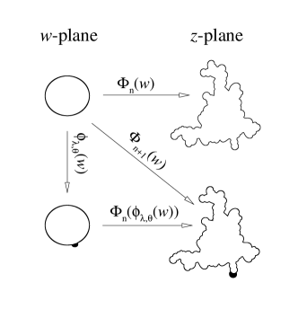
Figure 1: A circle in the $w$-plane is mapped to a $\mathcal{C}_{n}$ in the $z$-plane by $\Phi_{n}(w)$. The same function maps a circle with a bump at $\theta_{n+1}$ to a $\mathcal{C}_{n+1}$.

In this paper our analysis is based on the boundary of the clusters and we need to have a uniform data on the boundary. This can be done formally by using a uniform series of $\left\{\beta_{s}\right\}_{s=1}^{S}$ during the conformal mapping from a unit circle to the boundary of the cluster i.e., $\left\{w_{s}=e^{i\beta_{s}}\right\}_{s=1}^{S}$. This procedure can not be applied operationally, because in order to have a reasonable data in the fjords, one has to set $S\gg n$ which needs very long simulation time.
Barra et al., Ref10 have focused on the branch points of the map and introduced another approach for selecting the series $\left\{\beta_{s}\right\}$. Following their approach, we define $w_{n}^{R}$ and $w_{n}^{L}$ as ”Right” and ”Left” branch points of the function $\phi_{\lambda_{n},\theta_{n}}$ in the following map, respectively

$$e^{i\alpha_{n}^{R,L}}=\phi_{\lambda_{n},\theta_{n}}(w_{n}^{R,L}),$$ (11)

where $|\alpha_{n}^{R}-\alpha_{n}^{L}|/2\pi$ is the fraction of the unit circle covered by the bump. Each new bump creates two new branch points on the boundary and in case of probable overlapping with previous branch point, some of the older ones will be removed. So the maximum number of branch points will be $2n$. If $w_{k}^{R,L}$ be a branch point of the $k$th bump without overlapping by the next $(n-k)$ bumps, it would be an exposed branch point of the map $\Phi_{n}$ but the pre-image of the branch on the unit circle will change from $w_{k}^{R,L}$ to $w_{k,n}^{R,L}$

$$\Phi_{k}(w_{k}^{R,L})=\Phi_{n}(w_{k,n}^{R,L}),$$ (12)

such that

$$w_{k,n}^{R,L}=\phi_{\lambda_{n},\theta_{n}}^{-1}\circ\cdots\circ\phi_{\lambda_{k+1},\theta_{k+1}}^{-1}\left(w_{k}^{R,L}\right).$$ (13)

The solvability of Eq. 13 determines whether the branch point remains exposed, and then by mapping them one gets a reasonable image of the fjords.

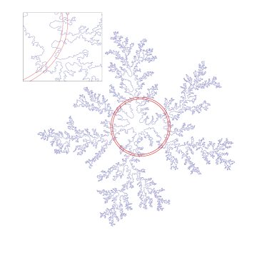
Figure 2: Boundary of a typical simulated DLA cluster consisting of $N=10^{5}$ bumps generated by using the HL algorithm, with $a=\frac{1}{2}$. The plotted shell is used to study the muliscaling properties of the boundary in Sec. V. The width of the shell is magnified by a factor of $10$. Inset: a close-up view of the cluster.

III Simulation

The simulation of the boundary of DLA clusters of different sizes is carried out using the algorithm discussed in the previous section. We set the parameter $a=\frac{1}{2}$, for which the function $\phi_{\lambda,\theta}(w)$ is analytically invertible.

At the $n$th step, $\theta_{n}$ and $\lambda_{n}$ are determined as follows. $\theta_{n}$ is selected from a uniform distribution in the range $[0,2\pi]$, and then $\lambda_{n}$ is computed using the Eq. 9. After determination of $\lambda$s and $\theta$s and computing exposed branch points $w_{k,n}^{L,R}$, together with Eq. 6, the boundary of each cluster is determined.
We generated $2000$ clusters of number of bumps $10^{3}\leqslant N\leqslant 5\times 10^{4}$ and $200$ clusters of $N=10^{5}$. A typical growth cluster is shown in Fig. 2. All average quantities which will be discussed later are taken over the simulated cluster ensemble.

IV Direct cluster analysis

In this section we do some direct measurements based on the geometry of clusters obtained from simulation. These include computation of the fractal dimension of generated DLA clusters and size-dependence of the variance of gyration radius of the clusters. We find a good agreement between our results and ones obtained from the analytical approach in Ref11 ; Ref11- . We also measure the density correlation function$-$which, to our knowledge, has not been computed yet for the HL method$-$ and we investigate its dependence on the size of the cluster. We find that the large-size behavior of the function corresponds to an expected correlation exponent $\alpha$ which is in a good agreement with the computed fractal dimension.

IV.1 Scaling of Gyration Radius for DLA Cluster

The fractal dimension $D_{c}$ of DLA clusters generated by HL method has been previously computed from the Laurent expansion of the conformal map, cf. Eq. 6, equal to $D_{c}=1.713(3)$ Ref11 ; Ref11- . The error in the last digit is indicated in parentheses. This has been obtained from the scaling relation between the first coefficient of the Laurent series of $\phi_{n}(w)$ and the size of DLA cluster.
Since the first coefficient is proportional to the radius of the cluster, this motivates us to measure the fractal dimension directly using the scaling relation between the average gyration radius $R^{c}_{g}$ of the cluster and the number of bumps $-$or equivalently the cluster size$-$ $N$, i.e., $R^{c}_{g}\sim N^{\nu_{c}}$, where $\nu_{c}=1/D_{c}$.
The result is shown in Fig. 3(a). We find that $\nu_{c}=0.581(2)$, in good agreement with previous results.

Another important result pointed out in Ref12 is the sharpness of the distribution of the first laurent coefficient. It has been shown numerically that the rescaled distribution width of squared first-laurent coefficient tends to zero as $N$ goes to infinity. Here, we check the same idea for the gyration radius of the clusters. The standard deviation of gyration radius is calculated from $\sigma^{c}=\sqrt{\langle{R^{c}_{g}}^{2}\rangle-\langle R^{c}_{g}\rangle^{2}}$, where $\langle\cdot\rangle$ denotes the ensemble average over simulated clusters of size $N$. The rescaled $\sigma^{c}$ as a function of $N$ is plotted in Fig. 3(b). As can be seen from this figure the fluctuation tends to zero for larger cluster size. This suggests that the rescaled distribution function of gyration radius of the clusters tends asymptotically to a $\delta$ function.
In order to investigate the asymptotic scaling behavior of $\sigma^{c}$, we proceed in the same way as Ref13 ; Ref9 , where the authors suggest that all of the length scales $\ell$ in DLA have a scaling relation with $N$, like

$$\ell\sim N^{1/D}(a+bN^{-\varphi})$$ (14)

with a single universal exponent $\varphi=0.33(6)$.
Our computation shown in Fig. 3(c) agrees with this scaling relation but with a different exponent of $\varphi=0.45(5)$, indicating that in the limit $N\rightarrow\infty$, the fluctuation of gyration radius has an asymptotic scaling behavior as that of the gyration radius, and nevertheless, the exponent seems not to be universal (this will be confirmed again in the following section for other length scales).

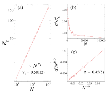
Figure 3: (a) The average gyration radius of clusters $R_{g}^{c}$, versus the number of bumps $N$. (b) Rescaled standard deviation of gyration radius $\sigma^{c}/R^{c}_{g}$ versus $N$. (c) Rescaled standard deviation of gyration radius ($\sigma^{c}/N^{1/D}$, $D=1.711$) versus $N^{-\varphi}$. The error bars are almost in the same size as the symbols.

IV.2 Density Correlation Function

In this subsection, we compute the two-point correlation function $c(\textbf{r})$, defined as

$$c(\textbf{r})=\frac{1}{V}\sum_{\textbf{r}^{\prime}}{\rho(\textbf{r}+\textbf{r}^{\prime})\rho(\textbf{r}^{\prime})},$$ (15)

where $\rho(\textbf{r})$ is density at position r, and the average is taken over all the points that belong to the cluster. For isotropic clusters the density correlation depends only on distance $r$.
For self-similar fractals, $c(r)$ should have the scaling form of $c(r)\sim r^{-\alpha}$, where the exponent $\alpha$ is named co-dimensionality and is equal to $\alpha=d-D_{c}$, where $d$ is the embedding dimension.

Operationally, we proceed as follows to determine the function $c(r)$. For each sample in the ensemble of clusters of a fixed size, we cover the cluster by a two dimensional square lattice. Then for each lattice site belonging to the cluster, we consider an annulus around it with mean radius of $r$ and thickness of a lattice spacing. The density of the cluster points in the annulus is then proportional to the two-point correlation function at distance $r$. The average is then taken over both all lattice points in the cluster and all clusters in the ensemble. This procedure is repeated for annulus of different mean radius.
We find that, for intermediate distances, the function $c(r)$ exhibits a power-law behavior with an exponent $\alpha$ depending on the cluster size $N$. This behavior is shown in Fig. 4 for three different sizes. The values of the exponent $\alpha$ as a function of the inverse size of the cluster is depicted in the inset of Fig. 4. In order to determine the value of the exponent in the large-size limit, we fit a polynomial curve to the data. We find that it extrapolates to $\alpha=0.29(1)$, whose value is checked not to be affected by the degree of the fitted polynomial. This value is in good agreement with the aforementioned relation $\alpha=d-D_{c}$, with $D_{c}\sim 1.71$.

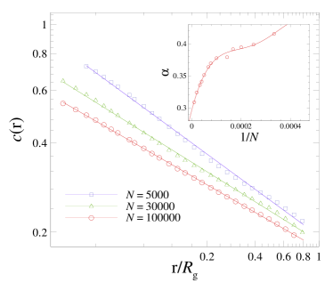
Figure 4: Two-point density correlation function $c(r)$ for three different cluster sizes $N$. The difference in the slope of the solid lines indicates the size dependence of the correlation exponent $\alpha$. The graph for $N=10^{5}$ is shifted downward by $0.12$. Inset: the exponent $\alpha$ versus $1/N$. The solid line is a polynomial fit of order $5$, which yields the asymptotic value of $\alpha=0.29(1)$. The error bars are almost in the same size as the symbols.

V Boundary Analysis

In this section, we study the scaling properties of various length scales related to the boundary of DLA clusters produced by HL method. We find that the fractal dimension of the boundary is the same as the DLA cluster, in agreement with the same conclusion reported in Ref14 , for DLA clusters produced according to the original definition. We also check the simple scaling relation Eq. 14 for various length scales including the gyration radius $R_{g}^{b}$, maximum radius $R_{max}$ and width $R_{w}$ of the boundary and their fluctuations. We find that all these length scales do not obey the scaling form Eq. 14 with a single exponent $\varphi$.
Finally, we check the multiscaling hypothesis for the boundary of the clusters and we will present evidence pointing to the existence of such anomalous scaling.

V.1 Scaling of boundary characteristic lengths

Each cluster boundary is divided into segments such that $i$th segment has a length $l_{i}$, and the distance of the midpoint of the segment from the center of mass is denoted by $R_{i}$. During the calculations, this procedure attributes a weight of $l_{i}$ to each distance $R_{i}$ and measures the following length scales in a more delicate manner.

V.1.1 Gyration radius of the boundary, $R_{g}^{b}$

The gyration radius of the boundary $R_{g}^{b}$ is defined by $R_{g}^{b}=\sqrt{\frac{1}{L}\sum_{i}{l_{i}R_{i}^{2}}}$, where $L$ is the total length of the boundary, and the sum runs over all segments on it. The fractal dimension of the boundary $D_{b}$ can be measured by using the scaling relation $R_{g}^{b}\sim L^{\nu_{b}}$, where $\nu_{b}=1/D_{b}$. Fig. 5 shows the ensemble average of gyration radius versus the average length of the boundary. We find that $\nu_{b}=0.587(4)$. This indicates that within the statistical errors, a DLA cluster generated by HL method and its boundary have a same fractal dimension i.e., $\nu_{c}=\nu_{b}$. This result is the same as one obtained before for DLA patterns grown according to the original definition Ref14 . It may be considered as another evidence that the patterns generated by method of iterated conformal maps proposed by Hastings and Levitov agree statistically with ones originally introduced by Witten and Sanders. We have also checked the scaling of $R_{g}^{b}$ with the cluster size and we found the same behavior as $R_{g}^{c}$ with $N$.
The inset of Fig. 5 shows the plot of the rescaled standard deviation of $R_{g}^{b}$ i.e., $\sigma^{b}/N^{1/D_{c}}$ against $N^{-\varphi}$. We find that $\varphi=0.31(5)$, in agreement with Eq. 14.

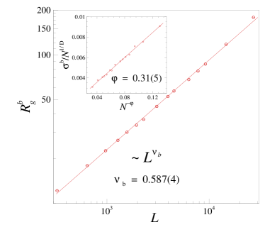
Figure 5: Average gyration radius of the boundary $R^{b}_{g}$, versus the average length of the boundary $L$. Inset: rescaled standard deviation of the gyration radius ($\sigma^{b}/N^{1/D}$, $D=1.711$) versus $N^{-\varphi}$. The error bars are almost in the same size as the symbols.

V.1.2 Maximum radius of the boundary, $R_{max}$

The other length scales we discuss here, are the lengths related to the maximum value of $R_{i}$ in each cluster boundary represented by $R_{max}$ in Fig. 6. We observe from Fig. 6(a) that the ensemble average of $R_{max}$ scales with size $N$, with $\nu_{max}=0.571(1)$, different from the gyration radius exponent. As shown in Fig. 6(b), the rescaled $R_{max}$ follows the simple scaling behavior of Eq. 14, with a quite different exponent of $\varphi=0.18(5)$ from the proposed universal value of $\varphi=0.33(6)$ in Ref13 ; Ref9 . We also checked this simple scaling behavior for the rescaled standard deviation of $R_{max}$, in agreement with Eq. 14 (see Fig. 6(c)).

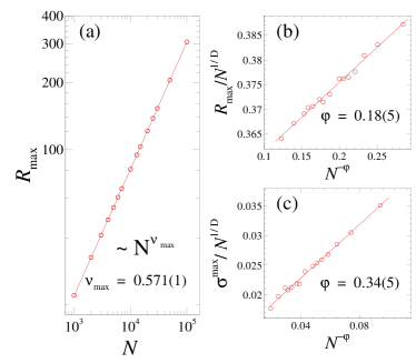
Figure 6: (a) The ensemble average of the most-far boundary segment from the seed $R_{max}$, versus the number of bumps $N$. (b) Rescaled $R_{max}$ (i.e., $R_{max}/N^{1/D}$, $D=1.711$), versus $N^{-\varphi}$. (c) Rescaled standard deviation of $R_{max}$ (i.e., $\sigma^{max}/N^{1/D}$, $D=1.711$) versus $N^{-\varphi}$. The error bars are almost in the same size as the symbols.

V.1.3 Interface width, $R_{w}$

According to the analogy between the DLA growing cluster and non-Euclidean growing interfaces, the interface width $R_{w}$ can be defined by $R_{w}=\sqrt{\frac{1}{L}\sum_{i}{l_{i}(R_{i}-\bar{R})^{2}}}$, where the mean radius of the cluster is $\bar{R}=\frac{1}{L}\sum_{i}{l_{i}R_{i}}$.
The growth exponent $\beta$ can be obtained from the evolution of the interface width $R_{w}\sim N^{\beta}$. As shown in Fig. 7(a), we obtain the growth exponent for DLA clusters generated by HL method equal to $\beta=0.557(2)$. We checked the correction to scaling for the exponent, according to Eq. 14 represented in Fig. 7(b), and we conclude that no correction exists. The fluctuation of the interface width (see Fig. 7(c)) exhibits a simple scaling relation of form Eq. 14, with a correction to scaling exponent of $\varphi=0.58(5)$. This exponent is very different from those obtained for hitherto mentioned length scales, and far from its proposed universal value.

The scaling properties of the interface width, apparently deviates from the simple scaling of Eq. 14, which has been proposed in Ref9 on refuting the multiscaling property of DLA cluster. The deviations of these boundary related length scales from the simple scaling behavior, motivated us to check an extension of the multiscaling property (previously applied for the mass of DLA clusters) to the length of the perimeter of clusters.

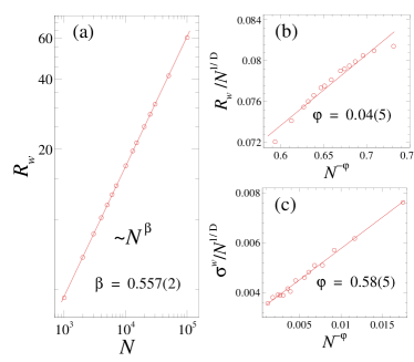
Figure 7: (a) The average interface width of the boundary of cluster $R_{w}$, versus the number of bumps $N$. (b) Rescaled interface width (i.e., $R_{w}/N^{1/D}$, $D=1.711$) versus $N^{-\varphi}$. (c) Rescaled standard deviation of the interface width (i.e., $\sigma^{w}/N^{1/D}$, $D=1.711$) versus $N^{-\varphi}$. The error bars are almost in the same size as the symbols.

V.2 Multiscaling analysis of the boundary of DLA clusters

In this section, we extend the concept of multiscaling, previously used for the mass of the DLA clusters Ref15 ; Ref16 ; Ref17 ; Ref18 (1998), to the length of the border of DLA. Our measurement for the perimeter of DLA clusters of size up to $10^{5}$ particles (or bumps), reveals the multiscaling behavior of the border.
For each cluster size, we generated an ensemble of DLA clusters by using the HL method and the perimeter of each sample has been determined as described in Sec. II. We proceed as follows: for each sample perimeter in the ensemble of size $N$ and average gyration radius of $R_{g}^{b}$, a shell of radius $r$ and of width $dr$ (which is about the linear size of a bump) is drawn (see Fig. 2 for illustration). Then we measure the density profile $g\left(r,R_{g}\right)$ defined as

$$g\left(r,R_{g}\right)dr=dl,$$ (16)

where $dl$ is the total length of the boundary within the shell of radius $r$.

The plot of $g\left(r,R_{g}\right)$ as a function of the rescaled radius $x=r/R_{g}^{b}$, within $0.1\leq x\leq 2$, is shown in Fig. 8 for four different sizes. This function has a maximum for distances around the gyration radius of the cluster. Assuming the scale invariance of the density profile Ref16 , the multiscaling exponent $D(x)$ can be defined as

$$g\left(r,R_{g}\right)=C(x)R_{g}^{D(x)-1},$$ (17)

where $C(x)$ is a scaling function. Thus, the multiscaling exponent can be obtained using the following relation

$$D(x)=1+\left.\frac{\partial\ln g\left(r,R_{g}\right)}{\partial\ln R_{g}}\right|_{x}\,.$$ (18)

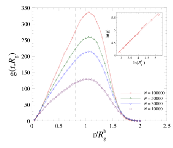
Figure 8: Examples of the density profile of the boundary length of the clusters within a shell of rescaled radius $x=r/R_{g}^{b}$, represented for four different sizes. Inset: log-log plot of the density profile at a certain rescaled radius of $x=r/R_{g}^{b}=0.8$ (the dashed line in the main figure). The slope of the fitted solid line yields $D(x=0.8)=1.67$ for $N=100000$. This figure summarizes the procedure we applied to obtain the functions $D(x)$ in Fig. 9. The error bars are almost in the same size as the symbols.

The inset of Fig. 8 shows the procedure we used to determine the multiscaling exponent as a function of $x$. At each $x$, the values of the density profile are read from Fig. 8 for each cluster size of gyration radius $R_{g}^{b}$, and then $D(x)$ is determined by Eq. 18.

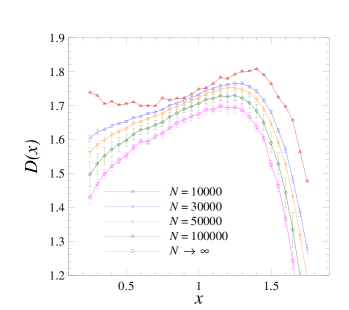
Figure 9: Multiscaling fractal dimension D(x) of the boundary for different cluster sizes as a function of $x=r/R_{g}^{b}$.

The whole behavior of $D(x)$ for different size intervals is shown in Fig. 9. This shows that the function $D(x)$ does not tend to a constant value as size increases, and there is a maximum around $x\simeq 1.2$ whose location does not depend on the size of cluster. Using the curves of Fig. 9 (and other similar curves obtained for other cluster sizes which not shown in the figure), we also estimated the value of $D(x)$ at each $x$ in the limit of $N\rightarrow\infty$. As shown in Fig. 9, $D(x)$ is not constant and varies with $x$, suggesting a multiscaling behavior. We therefore conclude that the perimeter of the DLA clusters generated by HL method does not have simple scaling, and thus a set of scaling exponents is needed to be described.

VI Conclusion

We studied scaling properties of DLA clusters generated by the Hastings-Levitov method. First, we calculated the fractal dimension of the clusters by direct analyzing of the DLA patterns in agreement with the previous results. We also computed the two-point correlation function of the mass of the cluster, and we found that in the large-size limit, it agrees with the obtained fractal dimension.

In the second part of the paper, we focused on the border of the DLA clusters and we investigated their scaling properties. We found that the fractal dimension of the perimeter is equal to that of the cluster. We checked the simple scaling behavior for various length scales including the gyration radius, maximum radius and the interface width of the boundary, together with their fluctuations. We found that all of these length scales do not have a simple scaling with a universal correction to scaling exponent. The growth exponent has been obtained from the evolution of the interface width. Finally, we found that the perimeter of DLA displays an asymptotic multiscaling property.

References

- (1)
- Witten, T.A. et al. (1981) T.A. Witten and L.M. Sander, Phys. Rev. Lett. 47 1400. (1981)
- Niemeyer et al. (1984) L. Niemeyer, L. Pietronero, H.J. Wiesmann, Phys. Rev. Lett. 52 1033. (1984)
- Brady et al. (1984) R.M. Brady and R.C. Ball, Nature (London) 309 225. (1984)
- Matsushita et al. (1984) M. Matsushita, M. Sano, Y. Hayakawa, H. Honjo, Y. Sawada, Phys. Rev. Lett. 53 286. (1984)
- Paterson et al. (1984) L. Paterson Phys. Rev. Lett. 52 1621. (1984)
- (7) M.B. Hastings and L.S. Levitov, Physica D 47 244. (1998)
- (8) A. Coniglio and M. Zannetti, Physica A 163 325. (1990)
- (9) E. Somfai, L.M. Sander, R.C. Ball, Phys. Rev. Lett. 83 5523-5526. (1999)
- (10) R.C. Ball, N.E. Bowler, L.M. Sander, E. Somfai, Phys. Rev. E 66 026109. (2002)
- (11) E. Somfai, R.C. Ball, N.E. Bowler, L.M. Sander, Physica A 325 19. (2003)
- (12) F. Barra, B. Davidovitch, I. Procaccia, Phys. Rev. E 65 046144. (2002)
- (13) B. Davidovitch and I. Procaccia, Phys. Rev. Lett. 85 3608. (2000)
- (14) B. Davidovitch, A. Levermann, I. Procaccia, Phys. Rev. E 62 R5919. (2000)
- (15) B. Davidovitch, H.G.E. Hentchel, Z. Olami, et al., Phys. Rev. E 59 1368-1378. (1999)
- (16) C. Amitrano, P. Meakin, H.E. Stanley, Phys. Rev. A 40 1713. (1989)
- (17) M. Plischke and Z. Racz, Phys. Rev. Lett. 53 415-418. (1984)
- (18) C. Amitrano, A. Coniglio, P. Meakin, M. Zannetti, Phys. Rev. B 44 4974. (1991)
- (19) B.B. Mandelbrot and B. Kol, Phys. Rev. Lett. 88 055501. (2002)
- (20) A.Y. Menshutin and L.N. Shchur, Phys. Rev. E 73 011407. (2006)