Optical and near infra-red colours as a discriminant of the age and metallicity of stellar populations

Abstract

We present a comprehensive analysis of the ability of current stellar population models to reproduce the optical ($ugriz$) and near infra-red ($JHK$) colours of a small sample of well-studied nearby elliptical and S0 galaxies. We find broad agreement between the ages and metallicities derived using different population models, although different models show different systematic deviations from the measured broad-band fluxes. Although it is possible to constrain Simple Stellar Population models to a well defined area in age-metallicity space, there is a clear degeneracy between these parameters even with such a full range of precise colours. The precision to which age and metallicity can be determined independently, using only broad band photometry with realistic errors, is $\Delta{[Fe/H]}\simeq 0.18$ and $\Delta{\log{Age}}\simeq 0.25$. To constrain the populations and therefore the star formation history further it will be necessary to combine broad-band optical-IR photometry with either spectral line indices, or else photometry at wavelengths outside of this range.

1 Introduction

Knowledge of the star formation history of galaxies is key to our understanding of their formation and of environmental influences upon their properties. However, the relationship between observable quantities and the fundamental parameters of the stellar population is complex. Observables are usually interpreted by comparison with single-age, single-metallicity population (Simple Stellar Population or SSP) models. An SSP model is derived from a set of stellar tracks and isochrones, which are populated using an assumed Initial Mass Function (IMF). Empirical or theoretical spectra are summed along the isochrone, with appropriate weighting, producing the SSP spectral energy distribution. These Isochrone Synthesis Models were refined by Charlot & Bruzual (1991), and Bruzual & Charlot (1993) and found broadly to reproduce both spectroscopic and photometric properties of galaxies. However in detail the predictions are affected in a complex way by the population age, metallicity, abundance ratios such as the degree of enhancement of $\alpha$-elements relative to solar ratios, and the IMF. Interpretation of gradients within individual galaxies, or trends with global parameters such as galaxy luminosity amongst samples, for instance in clusters, are subject to various degeneracies of which the best known is that between age and metallicity for old populations (Worthey 1994; Kodama & Arimoto 1997).

Most attempts to break these degeneracies, and establish luminosity-weighted stellar ages, metallicities and abundance ratios have involved obtaining high quality spectra of individual galaxies. A common technique is to compare plots of pairs of line indices with model grids (e.g. Trager et al. 2000a,b, 2008; Kuntschner et al. 2001; Poggianti et al. 2001a,b; Nelan et al. 2005; Sánchez-Blázquez et al. 2006). Other authors define combinations of indices designed to measure specific parameters (Vazdekis & Arimoto 1999), or apply Principal Component Analysis or other non-parametric techniques to extract specific physical parameters from galaxy spectra (Panter et al. 2003, 2007; Tojeiro et al. 2007; Ocvirk et al. 2006a,b; Koleva et al. 2008). An alternative which represents a compromise between analysis of high signal-to-noise spectra, which can necessarily be applied only to limited samples, and broad band photometry, is the technique of narrowband continuum photometry (Rakos et al. 2007, 2008).

These techniques are limited to bright galaxies, where spectra or narrow band images of sufficiently high signal-to-noise ratio can be obtained. For fainter samples, of dwarf or high redshift galaxies, or of star clusters associated with brighter galaxies, it is important to establish how precisely stellar population parameters can be measured from broad-band photometry alone. Optical broad-band photometry alone cannot break the age-metallicity degeneracy (e.g. Kodama and Arimoto 1999), however extending the spectral range appears to provide additional constraints. This has been demonstrated for optical - near infra-red colours by several studies, starting with Bothun et al. (1984) who argued that $J-K$ depends principally on metallicity, while $B-H$ depends also on mean stellar age. The same colour combination was used used by Bothun & Gregg (1990) in an investigation of the star formation history of S0 galaxies. Peletier, Valentijn and Jameson (1990) used $U-B$, $B-V$ and $V-K$ colours; Peletier & Balcells (1996) $U-R$ vs. $R-K$; Bell & de Jong (2000) $B-R$ vs $R-K$; and James et al. (2006) $B-K$ vs. $J-K$ in further studies of the metallicities and star formation histories of unresolved stellar populations in galaxies. Some success has also been found in the use of optical-ultraviolet colours, with Kaviraj et al. (2007a,b) combining SDSS optical and GALEX ultraviolet photometry in a study of the star formation histories of low-redshift early-type galaxies.

One of the problems with all of these techniques is the model-dependence of the results. Each of the studies discussed above will use a specific set of stellar tracks and isochrones, and a specific set of theoretical or empirical spectra. Differences between the results of these studies are often the result of differences between models rather than between observations. In this paper we use a variety of popular SSP models to derive stellar population parameters from accurate photometry in ($ugrizJHK$) passbands of a sample of nearby E/S0 galaxies. By using well calibrated public datasets (SDSS and 2MASS) and photometry in consistent, well-defined apertures, the observational error is reduced and we can investigate in detail the uncertainty caused by the modelling process, the differences between popular sets of models, the difference between scaled-solar and $\alpha$-enhanced models, and that caused by different assumptions about the foreground extinction. Moreover for some galaxies our derived parameters can be compared directly with spectroscopic studies (e.g. Trager et al. 2008).

A somewhat similar study has been carried out by Eminian et al. (2008). These authors use public catalogue photometry in optical and near-infrared bands for a sample drawn from the SDSS spectroscopic catalog. Their study contains a high proportion of currently star forming galaxies, and their focus is on the correlation between star formation, dust, and near-IR colours, rather than the age and metallicity of old populations. Their study relies on magnitudes from two different catalogue sources with different effective apertures, so while they use colours internal to each of the datasets (e.g. $g-r$ and $Y-K$) they cannot use the SED over the entire range to constrain the population. The much lower precision of their photometry of individual galaxies is balanced by the much larger sample that they use.

Conroy et al. (2009) use a new set of SSP models, currently unavailable to us, to model the broad band SDSS and 2MASS catalogue magnitudes of samples of galaxies at low redshift and at redshift $\sim$2. They emphasise the importance of understanding the Thermally Pulsing Asymptotic Giant Branch (TP-AGB) phase of stellar evolution and of the IMF, and examine the effect of both on broad-band colours. They find that Horizontal Branch morphology impacts the derived population parameters less than either the TP-AGB and the IMF. They also conclude that the evolution of a multi-metallicity population, particularly in passbands at wavelengths longer than $V$, is equivalent to that of a single-metallicity population whose metallicity is the mean of the multi-metallicity population. The study of Conroy et al. (2009), as with that of Eminian et al. (2008), relies on large samples of galaxies with individually much lower photometric precision than that of our measurements.

Lee et al. (2007), in a study which focuses on the composite populations found in spiral galaxies, find that because the youngest population ($<$ 2 Gyr) dominates the light, broadband colours can partially break the age-metallicity degeneracy. However at older ages they find large scatter in the results obtained from models by different authors.

A complementary approach is to apply similar techniques to extragalactic star clusters, in particular to the globular cluster populations of galaxies. This has the advantage that, although the cluster populations associated with galaxies can have multiple formation epochs and particularly metallicities, an individual cluster is more likely than a galaxy to contain stars of only a single age and metallicity. This is balanced against the disadvantage of using star clusters, that a comparatively small number of bright stars (on the AGB or on the upper main sequence, depending upon the age of the cluster) will contribute substantially to the luminosity, and that statistical fluctuations in these numbers will cause fluctuations in the photometry, and thus lead to additional uncertainty in the derived parameters of the stellar population. This is not a problem for the galaxies in our study, which will have typically $10^{4}$ times as many stars in our defined apertures.

Puzia et al. (2002), and Hempel & Kissler-Patig (2004a) applied $V-I$ vs. $V-K$ colour-colour plots to the study of unresolved stellar populations in globular clusters, in order to distinguish the metallicities of the separate cluster populations associated with the parent galaxies. Hempel & Kissler-Patig (2004b) add $U$ band observations and show that the age resolution is enhanced, enabling separate formation epochs to be distinguished as well. Kundu et al. (2005) find a substantial intermediate age population associated with the Virgo elliptical galaxy NGC4365, using $gIH$ photometry alone.

Anders et al. (2004) examine the ability of broad band ($UBVRIJH$) photometry to recover the age and metallicity of artificial clusters generated with GALEV SSP models (Schulz et al. 2002). They set observational errors to be 0.1 mag in all passbands in their study, which is a somewhat larger value than we have in our observational data. They find that the $U$ and $B$ bands are critical for determining ages, and that the maximum available wavelength range is also important. Applying the same fitting technique to a sample of real clusters, de Grijs et al. (2005) find that for young star clusters, and now using HST filters and passbands, the estimates for the cluster age have an approximately Gaussian distribution with $\sigma_{log(t)}\leq 0.35$. They do not attempt to constrain the metallicity of their clusters, but note that the effects of uncertainties in metallicity and extinction on the age determined are small.

Most of the Globular Cluster studies also rely on only one set of stellar population models, usually those of Bruzual & Charlot (2003, hereafter BC03). However Hempel et al. (2005), in their appendix, compare the model predictions for ($V-I$) and ($V-H$) for BC03 models and those of Maraston (2005), and find that the predictions for these colours do not differ significantly except for metal poor populations with age $\leq$ 2Gyr. Pessev et al. (2008) present 2MASS-based JHK photometry of a sample of Magellanic Cloud globular clusters, and combine this with $UBV$ photometry from the literature to undertake a comparison of the performance of four sets of stellar population models at distinguishing age and metallicity for this sample. They find that all models reproduce the colours for old clusters quite well, but that for young ages there are more substantial differences. Overall they conclude that the models of BC03 give the best quantitative match to their data. This study is carried out at lower metallicity than ours, but comparison with our conclusions will be interesting nevertheless.

2 Observational Data

Our sources of observational data are the image servers provided by data release 6 of the Sloan Digital Sky Survey (SDSS; Adelman-McCarthy et al. 2008) and by the 2 Micron All-Sky Survey (2MASS; Skrutskie et al. 2006). We have chosen a sample of bright galaxies in the Coma cluster, and a sample at intermediate luminosity from the Virgo cluster to test our techniques. These samples are limited by practical issues: for fainter galaxies in Coma the photon and read noise, which are the dominant noise source in our 2MASS magnitudes, adversely affect the precision, while for brighter galaxies in Virgo the galaxy image is so large that it is impossible to determine sky levels on the size of image provided by the SDSS image server. To sample a range of absolute magnitude it was necessary to select galaxies from both clusters.

SDSS and 2MASS images of a number of galaxies were downloaded from the image servers, and a sample of galaxies was chosen. In the Coma cluster, as many galaxies as possible in common with the sample of Trager et al. (2008) were selected. In Virgo, galaxies were chosen where possible to be in the sample of the ACS Virgo cluster survey (Côté et al. 2004) and the catalogue of Michard (2005), note however that the majority of Michard’s sample are too large for this study. Galaxies were rejected from the sample if they fell too close to an image boundary, to a neighbouring galaxy, or to a superimposed star to allow definition of a clean circular aperture centred on the galaxy. The final sample contained 14 galaxies, eight from Coma and six from Virgo. In Table  1 we present the basic properties of this sample; galaxy types, redshifts and the Schlegel extinctions are taken from the NASA Extragalactic Database (NED), and the absolute V band magnitudes are taken from the Third Reference Catalogue (RC3, de Vaucouleurs et al. 1991), assuming distance moduli of 35.0 for Coma, and 31.1 for Virgo.

Table 1: Basic properties of the sample galaxies.

Galaxy	Type	Redshift	$A_{V}$	$M_{V}$
	(NED)		(Schlegel)	(RC3)
IC3501	d:E1	0.0055	0.092	–17.37
NGC4318	E	0.0041	0.083	–17.88
NGC4515	S0-	0.0032	0.103	–18.60
NGC4551	E:	0.0039	0.128	–19.21
NGC4564	E6	0.0038	0.116	–20.10
NGC4867	E3	0.0162	0.034	–20.57
NGC4872	SB0	0.0241	0.030	–20.62
NGC4871	SAB0/a	0.0227	0.030	–20.89
NGC4873	SA0	0.0194	0.027	–20.93
NGC4473	E5	0.0075	0.094	–20.99
NGC4881	E0	0.0225	0.036	–21.47
NGC4839	cD	0.0246	0.032	–22.97
NGC4874	cD	0.0241	0.028	–23.35
NGC4889	cD/E4	0.0217	0.032	–23.54

Notes to Table 1: Column 1 gives the galaxy name, column 2 the type from NED. Column 3 gives the redshift, again from NED, column 4 the extinction $A_{V}$ using the Schlegel (1998) maps. Column 5 is a $V$ band absolute total magnitude for the galaxy from RC3, using the distance modulus estimates given in the text. The IC3501 $M_{V}$ is determined from interpolation of $g$ and $r$ flux densities.

For each galaxy we measured aperture magnitudes in a series of apertures using the iraf task phot. Sky levels were determined in a number of regions of the image chosen to be free of foreground stars. Galaxy centres were determined in each image using the centroiding function within phot. For each galaxy we then chose an optimum aperture, in the range 20 – 40 arcsec diameter, within which to measure the magnitude in all passbands. All apertures are large enough that the different point spread functions of SDSS and 2MASS data do not have a significant effect. The optimum aperture chosen was in each case a compromise between the size of the galaxy, the proximity of neighbours, and the additional noise in the 2MASS magnitudes in larger apertures.

Magnitude zeropoints were taken directly from the fits headers of the 2MASS images, however for the SDSS data the zero point keyword (FLUX20) in the fits header of the downloaded image files (fpC files) has not been calculated using the final calibration information. Instead we recalibrated the fpC images using the zeropoint, extinction correction, and airmass given in the tsField files for the relevant Run and Field number. This recalibration gives a substantial correction to the magnitudes calculated using the image headers, particularly in the $u$, $g$ and $z$ bands where the corrections are in the range 0.05 – 0.1 magnitudes.

2.1 Homogenising galaxy photometry

In order to compare the models to our galaxy observations, the measured magnitudes must be homogenised to the same photometric system, for which we choose the AB magnitude system. Our optical photometry is carried out in the SDSS DR6 system, however there are sky position dependent differences between DR6 and DR7 zero points (see Padmanabhan et al. 2008). We transform our photometry to the DR7 photometric system by adding the difference between zero points calculated for each galaxy from the difference between DR6 and DR7 catalogue magnitudes. The SDSS DR7 photometry is brought onto the AB magnitude system by subtracting 0.04 from the $u$ and adding 0.02 to the $z$ band magnitudes as recommended on the SDSS web pages. We note that Eisenstein et al. (2006), in their work on hot white dwarfs, recommend a slightly different AB transformation vector, the main difference of which is to add approximately 0.015 to the $i$ band magnitudes. This vector might improve marginally many of our fits, however as the SDSS project appears not to have adopted the Eisenstein et al. transformation vector we do not feel justified in doing so.

The Infrared 2MASS magnitudes make use of the Vega magnitude system; these are brought on to the AB system by adopting the conversions from Cohen, Wheaton & Megeath (2003), shown in table 2. As a check we also convolved the $\alpha$ Lyræ (Vega) spectral energy distribution of Kurucz (1993) with the 2MASS $JHK_{s}$ response curves and converted the results to AB magnitudes, in effect calculating the magnitudes of Vega in the AB system. After taking into account the AB magnitude of Vega (0.03), our values are in agreement with those of Cohen, Wheaton & Megeath (2003).

Table 2: Conversions between 2MASS (Vega) and AB magnitude systems for the $JHK$ bands, taken from Cohen, Wheaton & Megeath (2003). To apply the corrections, $m_{AB}=m_{\rm Vega}+c$, where $c$ is the relevant correction from the table, shown to 3 decimal places. The uncertainties for each of the corrections are added in quadrature to the photometric errors in the $J$, $H$ & $K_{s}$ bands.

Band	$J$	$H$	$K_{s}$
Correction	0.894	1.374	1.840
Uncertainty	0.022	0.022	0.022

2.2 Photometric errors and corrections

For each magnitude we calculated an error, allowing for three sources of uncertainty. The first was the error in the measurement process, which in turn results from errors in the determination of the sky level. The measurement error was estimated from the SDSS and 2MASS images by repeated measurements of the magnitudes from the same image. In the 2MASS images this is a significant, albeit never dominant, source of error. The second source of error comes from noise in the image. This is calculated from the image gains given in the fits headers, and the image statistics as measured in the apertures in the case of SDSS passbands, and as given in the image headers in the case of 2MASS. For the 2MASS data the errors are corrected to allow for the resampling and smoothing applied to the data before delivery, using the prescription given on the 2MASS web pages.

The third source of error is the error on the photometric zero point, and this is taken from the web pages of SDSS and 2MASS respectively. For the 2MASS data we consider also the uncertainty in the conversion of 2MASS to AB magnitudes, as given in Table  2. These error sources are all added in quadrature. The zero point error always dominates for all SDSS passbands, whereas the image noise error dominates in most cases for 2MASS bands.

Magnitudes are not K-corrected, as the fitting procedure we use integrates the redshifted model flux over the rest wavelength filter passbands, however they are corrected for Galactic extinction, using the $A_{V}$ estimates of Schlegel et al. (1998), as tabulated in NED, and converted to SDSS passbands using the prescription of Kim and Lee (2007), and to $JHK$ using the Schlegel et al. prescription which is in turn derived from the functional form of Clayton & Cardelli (1988). The final magnitudes and errors used for the fitting are presented in Table 3.

3 Stellar Population Models

We have chosen to test seven popular sets of stellar population models against the data presented in Section 2. All models produce a series of synthetic spectra at points on a grid in age–metallicity space which are compared with the broad-band photometry as described in Section 4. For convenience, the basic parameters of each model are presented in Table 4, and we describe here briefly the further relevant details, in particular the treatment of the TP-AGB stars which are generally not included in the adopted stellar evolutionary tracks. We refer the reader to the original papers describing these models for a full description of each model.

1. Bruzual & Charlot (2003) models (BC03) use the Padova 1994 evolutionary tracks (Alongi et al. 1993; Bressan et al. 1993; Fagotto et al. 1994a,b; Girardi et al. 1996) with the TP-AGB and Post Asymptotic Giant Branch (PAGB) phases treated according to Vassiliadis & Wood (1993, 1994). We use the STELIB spectral library in our modelling, although our results do not change if we use the BaSeL-2.0 library. Neither stellar library contains carbon stars or upper TP-AGB stars and the spectra for these stars are constructed from observational libraries as described by BC03.

2. PÉGASE models (Fioc & Rocca-Volmerange 1997, 1999) also use stellar tracks from the Padova group, and pseudo-tracks for the TP-AGB phase as proposed by Groenewegen & de Jong (1993).

3. Starburst99 (Vázquez & Leitherer 2005) is of particular interest in the study of young stellar populations, although it is designed to model populations of any age. It uses the Padova 1994 stellar tracks and incorporates TP-AGB stars in a similar manner to BC03, as described by Vázquez & Leitherer (2005). Spectra were computed using the PAULDRACH/HILLIER option, which uses the BaSeL-2.0 atmospheres for all except the hottest stars. Starburst99 models using Geneva high mass-loss isochrones were also computed, but provided a very poor fit.

4. GALEV (Anders & Fritze-van Alvensleben 2003) is an evolutionary synthesis code written to study the spectral and chemical evolution of galaxies, underpinned by a set of SSP models (Schulz et al. 2002; Anders et al. 2004) using Padova isochrones and BaSeL-2.0 atmospheres.

5. The SPEED models are described by Jimenez et al. (1995, 2004) and adopt a stellar evolution code based upon Eggleton (1971, 1972) but with improvements, particularly in the modelling of the HB and AGB. Mass loss at the RGB tip is modelled using a distribution of values of the Reimers (1975) mass loss parameter $\eta$, and this distribution is calibrated against the observed HB morphologies of Galactic star clusters (Jimenez et al. 1996). The AGB is modelled as described by Jorgensen (1991). Spectra are largely taken from Kurucz (1993), but the authors compute their own LTE stellar atmosphere models for stars cooler than 4000 K.

6. Maraston (2005) presents a set of models determined from an evolutionary synthesis code (Maraston 1998) based upon the tracks of Cassisi et al. (1997a,b; 2000) for main sequence stars, and upon the Fuel Consumption Theorem (Renzini & Buzzoni 1986) for post-MS evolution, calibrated against clusters in the Magellanic Clouds.

   The BaSeL2.0 library of stellar spectra is used, with TP-AGB stars taken from Lançon & Mouhcine (2002). Maraston’s models are available with two horizontal branch morphologies (RHB and BHB) and we primarily consider the RHB models which are more appropriate for metal-rich populations. However, the existence of a blue HB morphology in a small number of metal-rich Galactic globular clusters (Busso et al. 2007) leads us to consider the BHB models as well.

   Maraston et al. (2008) discuss a set of related models which use the Pickles (1998) stellar library instead of BaSeL-2.0, but these were not available to us at the time of writing.

7. The BaSTI (Bag of Stellar Tracks and Isochrones) models are based on the work of Pietrinferni et al. (2004), extended to cover TP-AGB stars by Cordier et al. (2007). Model spectra are constructed from the BaSTI isochrones as described by Percival et al. (2008), using the ‘low resolution’ version of the model spectra. These are based upon the model atmospheres of Castelli & Kurucz (2003), supplemented by models from the BaSeL-3.2 library (Westera et al. 2002) for cool stars (T $<$ 3500 K), and by the empirical spectra of Lançon & Mouhcine (2002) for AGB carbon stars.

   Because these models are ‘in-house’, we are able to test different prescriptions for $\alpha$-enhancement and HB morphology. In addition to the scaled-solar models (Pietrinferni et al. 2004) we analyse also the [$\alpha$/Fe] = +0.4 models and isochrones of Pietrinferni et al. (2006). We also analyse two different values (+0.2 and +0.4) of the Reimers (1975) mass-loss parameter, $\eta$. Discussion of the effects of varying [$\alpha$/Fe] and $\eta$ is presented in Section 5.2

4 Integration and Fitting Procedures

4.1 Calculating model fluxes

In order to compare our observations with the results of SSP modelling, we convert from our observed AB magnitudes and magnitude errors to fluxes. To extract comparable fluxes, $S_{n}$, from the SSP SEDs of each species there are a number of steps. First, we multiply the wavelength values of the given SSP model by a factor of $(1+z)$ to account for the redshift of the galaxy in question. Second we rebin linearly the transmission function of each filter, $T_{\lambda,n}$, onto the wavelength scale of the models.

For each SSP SED $f_{\lambda}$, filter $n$, and filter transmission function $T_{\lambda,n}$, we then integrate the total flux in the passband using trapezoidal summation:

$$S_{n}=\frac{\displaystyle\int f_{\lambda}\lambda T_{\lambda,n}d\lambda}{\displaystyle\int\lambda T_{\lambda,n}d\lambda}$$ (1)

Next, we convert the observed AB magnitudes to $f_{\lambda}$ using:

$$f_{\lambda,n}=10^{(-m_{AB}/2.5)}\times f_{0}\times{c/\lambda_{eff,n}^{2}}$$ (2)

where $f_{0}$ is the AB magnitude zero point of 3631 Jy, and $\lambda_{eff,n}$ is the effective, or pivot, wavelength of the passband, defined by:

$$\lambda_{eff}^{2}={\int{T_{\lambda}\lambda d\lambda}\over\int{{T_{\lambda}\over\lambda}d\lambda}}$$ (3)

We are now in a position to compare our observations with the model SSP fluxes.

4.2 $\chi^{2}$ fitting

In order to quantify the extent to which the galaxies in our sample are described by the array of models mentioned in section 3, we employed a simple reduced $\chi^{2}$ test. For a given galaxy with observed fluxes $f_{i}$ with each flux having an associated error $\sigma_{i}$ in $n$ bands, the extent to which they are well described by a model with fluxes $S_{i}$ is approximated by the reduced $\chi^{2}$, calculated as follows;

$$\chi^{2}_{\nu}=\frac{1}{(n-\kappa)}~{}\sum_{i=0}^{n}\frac{(NS_{i}-f_{i})^{2}}{\sigma_{i}^{2}},$$ (4)

where $N$ represents the normalisation of the model magnitudes and $\kappa$ represents the number of constraints associated with the models. The normalisation factor $N$ is calculated by analytically solving the equation ${\rm d}\chi^{2}_{\nu}/{\rm d}N=0$. The value of $\kappa$ used for these calculations is 3, due to the treatment of a galaxy model’s age, metallicity, and flux density normalisation as free parameters. Model SSPs that approximate our galaxy observations well will then have values of reduced $\chi^{2}$ approaching unity, while for those models which do not approximate our observations well the values will be higher, depending on the ‘goodness of fit’.

In order to discriminate between the large numbers of models for a given galaxy, the best fit value of $\chi^{2}_{\nu}$ is calculated for every SSP in each model species (e.g. BC03, M05, etc.). In this way we build up a database of best-fit $\chi^{2}_{\nu}$ for all values of SSP age and metallicity for each galaxy in our sample. Making use of this database, we can then compare the results of our $\chi^{2}$ fitting to those of other studies (e.g. Trager et al., 2008). The properties of the best fit models to each of the galaxies in our sample are shown in tables 5 and 6.

5 Analysis

Table 3: BaSTI models for different $\alpha$-enhancement and mass loss parameters

	BaSTI
	$[{\alpha}/Fe]$ = 0.0, $\eta$ = 0.2			$[{\alpha}/Fe]$ = 0.0, $\eta$ = 0.4			$[{\alpha}/Fe]$ = 0.4, $\eta$ = 0.2			$[{\alpha}/Fe]$ = 0.4, $\eta$ = 0.4
	$\chi^{2}_{\nu}$	Age	$[{Fe\over H}]$	$\chi^{2}_{\nu}$	Age	$[{Fe\over H}]$	$\chi^{2}_{\nu}$	Age	$[{Fe\over H}]$	$\chi^{2}_{\nu}$	Age	$[{Fe\over H}]$
IC3051	1.61	4.50	–0.25	1.47	4.50	–0.25	1.04	8.50	–0.60	0.95	14.00	–0.60
NGC4318	1.65	8.00	–0.25	1.58	8.00	–0.25	1.56	13.50	–0.60	2.27	5.50	–0.29
NGC4515	2.66	6.00	–0.25	2.56	6.00	–0.25	2.67	10.00	–0.60	2.87	10.50	–0.60
NGC4551	2.62	2.75	0.40	2.50	2.75	0.40	2.76	7.50	–0.09	2.69	8.00	–0.09
NGC4564	2.78	3.00	0.40	2.71	3.00	0.40	1.31	6.50	0.05	1.40	10.00	–0.09
NGC4867	2.91	3.00	0.40	2.82	3.00	0.40	0.54	6.00	0.05	0.57	6.00	0.05
NGC4872	2.43	3.00	0.40	2.37	3.00	0.40	0.73	8.50	–0.09	0.74	9.00	–0.09
NGC4871	2.09	3.00	0.40	2.07	3.00	0.40	0.89	10.00	–0.09	0.86	10.00	–0.09
NGC4873	2.05	3.00	0.26	2.05	3.00	0.26	0.91	11.00	–0.29	0.99	11.00	–0.29
NGC4473	2.37	3.00	0.40	2.33	3.00	0.40	2.36	6.50	0.05	2.39	10.00	–0.09
NGC4881	2.60	3.00	0.40	2.54	3.00	0.40	0.77	6.50	0.05	0.78	10.00	–0.09
NGC4839	3.90	6.00	0.40	2.70	5.00	0.40	1.17	8.50	0.05	1.18	8.50	0.05
NGC4874	3.38	4.50	0.40	2.20	5.00	0.40	1.28	11.50	–0.09	1.31	12.00	–0.09
NGC4889	4.46	6.50	0.40	4.37	6.50	0.40	1.34	10.00	0.05	1.35	10.50	0.05

Notes to Table  3: Columns 2 – 13 - Best fitting BaSTI models for two values of $[{\alpha}/Fe]$, and for two values of the Reimers (1975) mass loss parameter $\eta$. For each combination of parameters, there are three columns in which we tabulate the best fit $\chi^{2}_{\nu}$, and the age (in Gyr) and [Fe/H] for the best fit model.

Remembering always that we are observing potentially composite populations, and comparing them with SSP models, we examine in turn the model sets, and how well they fit to the data.

1. BC03 models. The BC03 models often provide the lowest values of $\chi^{2}_{\nu}$ and thus objectively the best fit for the low luminosity Virgo galaxies in particular. In all cases this best fit comes from the [Fe/H] = 0.093 model, at an age between 2.5 and 12 Gyr, with the massive Coma galaxies in general showing the oldest ages. The residuals around the fit show a systematic pattern, in particular ($r-i$) is predicted too blue by 0.01 - 0.03 magnitudes for the lower luminosity Virgo galaxies, and 0.03 - 0.05 magnitudes for the more massive Coma galaxies. BC03 models provide too coarse a metallicity grid to investigate age-metallicity degeneracy, and in particular their one supersolar metallicity is [Fe/H] = 0.559, which is apparently too metal rich to fit any of our sample.

   In Figure  1 we show the dependence of $\chi^{2}_{\nu}$ on age, the best-fit model spectrum, and the residuals between data and best fit model, all for NGC4881, one of the best fitting galaxies. Similar plots for all galaxies and all model sets are available in the online data accompanying this paper.

2. PÉGASE models. These models provide higher values of $\chi^{2}_{\nu}$ than BC03, usually because they underpredict the flux in the $i$ band. PÉGASE models predict ($r-i$) to be too blue, and ($i-z$) to be too red, both by as much as 0.1 magnitude. The solar metallicity models show a minimum at generally slightly younger ages than BC03, but there is quite often a better fit from an interpolated model at [Fe/H] = –0.204 or +0.176. The $\chi^{2}_{\nu}$ curves for these models show clearly the age-metallicity degeneracy, where the supersolar model gives a fit a factor 1.5 – 2 younger, and the subsolar one a factor of $\sim$2 older.

3. Starburst99 models. Using Padova isochrones, these models give very similar results to PÉGASE, in that they predict the same ($r-i$) and ($i-z$) discrepancy, they show very similar ages, and the same age-metallicity degeneracy. They have less metallicity resolution than PÉGASE, and sometimes this results in a higher best value of $\chi^{2}_{\nu}$. Starburst99 models using Geneva isochrones fit substantially less well in all cases, and we do not consider these models further.

4. GALEV models. GALEV in general does not give quite as good a fit as PÉGASE, but the best fits usually occur at a similar age and metallicity. GALEV ages are similar to PÉGASE ages, and in general older than Starburst99 ages. These models again predict both ($r-i$) to be too blue and ($i-z$) to be too red, by 0.05 – 0.1 magnitude.

5. SPEED models. The best fit SPEED models are almost always old (often at their limit of 14 Gyr), and metal-poor (Z=0.001 or 0.004). They also overpredict the $u$ band flux by 0.1 mag or more, and as with other model sets predict ($r$ - $i$) to be too blue by 0.05 - 0.1 mag. The $\chi^{2}_{\nu}$ values are consequently high compared with other models.

6. Maraston (2005) models. The RHB models provide a less good fit to the broad band data than BC03, PÉGASE, Starburst99 or BaSTI, with $\chi^{2}_{\nu}<3$ for only two of the fourteen galaxies. The general pattern of the residuals is that ($r-i$) is predicted too blue, by 0.15 magnitude. For the Coma galaxies ($J-K$) is also too blue, by around 0.05 magnitude. The best fit ages are also uncomfortably young, in the range 1.5 – 3 Gyr even for massive cluster ellipticals. Such ages are in conflict with those derived from line indices (Trager et al. 2008). The BHB models are only appropriate for ages $>$ 10 Gyr and would generally be expected to fit low metallicity populations, so it is somewhat surprising that the [Fe/H] = 0.35 BHB model provides a better fit to the data than any of the RHB models, for the massive Coma galaxies in particular.

7. BaSTI models. The standard scaled-solar abundance models give slightly higher values of $\chi^{2}_{\nu}$ than BC03, and similar to PÉGASE or Starburst99. The residuals show an overprediction of the $r$ band flux, of 0.03 - 0.08 magnitudes. As with PÉGASE, BaSTI gives younger ages than BC03, largely because it has two supersolar metallicities ([Fe/H] = +0.26 and +0.40). In section  5.2 we discuss the effect of making different assumptions about [$\alpha$/Fe] and the Reimers (1975) mass loss parameter $\eta$, noting that we can only alter these parameters with the BaSTI models.

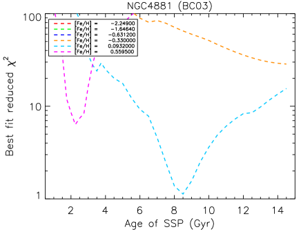
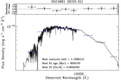
Figure 1: Left panel: $\chi^{2}_{\nu}$ against age for BC03 models of different metallicities as fit to the photometry of NGC4881. Lower right panel: the best fit model spectrum ([Fe/H] = 0.093; Age = 8.5 Gyr) with the SDSS and 2MASS passbands overplotted (blue horizontal error bars). Upper right panel: shows the residuals from the fit (data – model) in units of 0.1 magnitude

In Figure  2 we show $\chi^{2}_{\nu}$ at the best fit age and metallicity against absolute magnitude for our sample. There are some trends in some model sets, for instance the $\alpha$-enhanced models perform best for more luminous (and massive) galaxies, whereas BC03, PÉGASE, Starburst99 and BaSTI scaled-solar models perform better at lower luminosity.

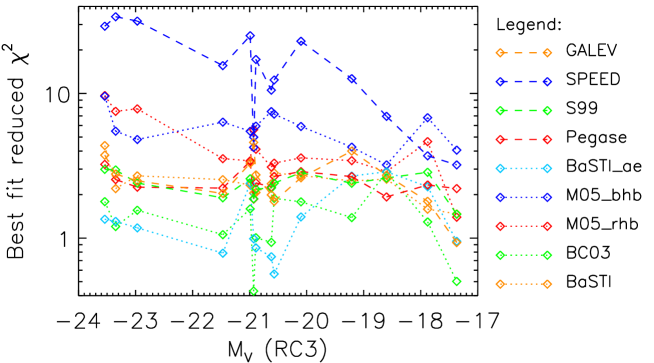
Figure 2: Best fit $\chi^{2}_{\nu}$ against absolute magnitude for each model set.

5.1 Age-metallicity degeneracy

BaSTI and PÉGASE models have sufficient metallicity resolution that for most galaxies, there are two, three or even four metallicities for which an age solution can be found with $\chi^{2}_{\nu}$ within 1.0 of the lowest. Table 7 presents these solutions. They have very different ages, and show the well known age-metallicity degeneracy in the sense that the highest metallicities give the youngest ages.

In Figure  3 we illustrate the close correspondence of the models of different age and metallicity for IC3501. For each model set, three models plotted in different colours, and shifted vertically to separate the traces. The values of [Fe/H] = –0.204 for PÉGASE and [Fe/H] = –0.25 for BaSTI provide the best fits. $\chi^{2}_{\nu}$ in each case is within 1 of the best fit, so the outer models, covering a metallicity range of $\simeq$ 0.4 in [Fe/H], and an age range of a factor two, cannot be ruled out.

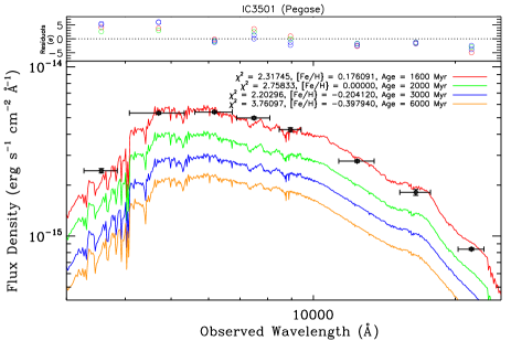
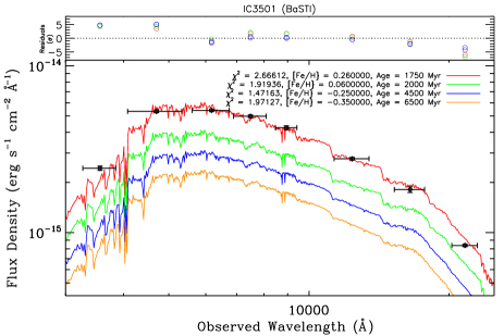
Figure 3: Illustration of the age-metallicity degeneracy, we show the best age fits at four metallicities for IC3501, using PÉGASE models (left panel) and BaSTI scaled-solar models (right panel). In each case the three older and more metal poor models are offset vertically, for clarity.

Independent of model set, we find the age and metallicity changes to be linked by the following relation:

$${{\delta{\log{Age}}\over{\delta{[Fe/H]}}}\simeq 1.2\pm 0.25}$$

Without other information to constrain metallicity or age, it appears that using broad band photometry from $u$ to $K$, we can measure these to $\Delta{[Fe/H]}\simeq 0.18$ and $\Delta{\log{Age}}\simeq 0.25$. Formal errors on the fitted age may be less than this for those model sets with a coarser metallicity grid, but these errors mean very little. Metallicities and ages can be constrained better by using line indices, with e.g. Trager et al. (2008) quoting errors of 0.02 – 0.15 dex on metallicity values and 0.04 - 0.20 dex on log(age) values derived using line indices alone.

The substantial errors on ages are disappointing, given the earlier claims that pairs of, for example, optical - near-infrared colours can break the age-metallicity degeneracy. Analysis of the colour-colour grids reveals why substantial errors should be expected, particularly for old stellar populations. In the BaSTI simple stellar population grids of $B-K$ vs. $J-K$ used by James et al. (2006), the $B-K$ colour, which is the principal age indicator, changes more between 3 and 5 Gyr than it does between 5 and 14 Gyr, and over the range 10-14 Gyr, the change in $B-K$ is typically only 0.02 – 0.03 mag. In addition, for high metallicity and old populations, increasing age leads to redder $J-K$ colours, so while the grid is not degenerate, the age and metallicity vectors are far from orthogonal. The same trends are found for the $V-I$ vs. $V-K$ grids of Puzia et al. (2002), which show a larger change in colours from 1 - 2 Gyr than from 5 – 15 Gyr. Thus, while such techniques can be very sensitive to the presence of even a small mass fraction of young or intermediate-age stars, the age discrimination for old populations is poor given typical photometric errors. Passbands blueward of our range may help (Kaviraj et al. 2006), as the models presented in Table 7 deviate from each other blueward of $u$, but uncertainties due to modelling of the Horizontal Branch become more serious.

This analysis emphasises, on the other hand, the importance of having models with sufficient age and metallicity resolution to identify the uncertainties in the derived parameters, and to investigate whether, for instance, the quality of the fits distinguishes between the fundamental parameters of the model sets, or whether the data demand more than an SSP to fit.

5.2 Abundance ratios and the morphology of the Horizontal Branch

The BaSTI [$\alpha$/Fe] = +0.4 models are the only $\alpha$-enhanced models that we investigate. For the Coma galaxies they provide better fits than any scaled solar models, occasionally excepting BC03, but for the lower-luminosity Virgo galaxies they are less successful. The pattern of residuals shows that the overprediction in $r$ is less than for the scaled-solar models, although they still predict ($r-i$) to be too blue, by 0.02 - 0.05 magnitude. However the main discrepancies are in ($u-g$), which is predicted too blue by 0.05 – 0.1 magnitude. The age-metallicity degeneracy still exists, with the three most metal rich models ([Fe/H] = –0.29, –0.09 and +0.05) showing minima with very similar values of $\chi^{2}_{\nu}$, but at ages which cover a range of a factor three, as can be seen in the fits to NGC4881 in the right panel of Figure  4. An extreme example can be seen in the left panel of this Figure, which shows the fits for IC3501. The metal-poor ([Fe/H]= –0.60 and –0.70), [$\alpha$/Fe] = 0.4; $\eta$ = 0.4 models fit very well at old ages due to a sharp transition from red to blue HB morphology at 8 – 14 Gyr. For other models this transition occurs at ages greater than the expected age of the universe. Using our broad-band photometry alone these models are almost indistinguishable from the $\sim$ 2 Gyr, [Fe/H] $\sim$ 0.29 models in this set (as Figure  4 shows), and from moderately metal-poor scaled-solar models. Similar effects are seen in the fits to NGC4318 and NGC4515.

In general, the best fit ages for the $\alpha$-enhanced models are greater than scaled-solar, with $\Delta({\rm log}Age)=0.34\pm 0.12$, a mean factor of two.

The Reimers (1975) mass-loss parameter $\eta$ has less effect, apart from in the metal-poor $\alpha$-enhanced models for the lowest mass galaxies discussed above. In other cases, when different metallicities have very close minimum $\chi^{2}_{\nu}$, changing $\eta$ will occasionally favour a different solution which, because of the age-metallicity degeneracy, will then have different age. For the [$\alpha$/Fe] = +0.4 models the $\eta$ = 0.2 solution can be one age step (500 Myr) younger at the same metallicity.

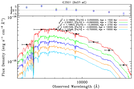
Figure 4: Age-metallicity degeneracy in the $\alpha$-enhanced models, we show the best age fits at five metallicities to IC3501. This is an extreme case, with an allowed age range of a factor 10, due to the transition in HB morphology at ages $>$ 8 Gyr in the high $\eta$, high [$\alpha$/Fe], low metallicity models. Again the older and more metal poor models are shifted vertically for clarity.

Maraston (2005) BHB models have very high values of $\eta$, between 0.45 and 1.0, and are designed to have a blue HB morphology even for metal-rich (0.5 – 2.0 solar) metallicities. These are available for very old populations (10 – 15 Gyr). The ages of the best fits are constrained to be old, and the best fit metallicities are in the range [Fe/H] = –0.33 to +0.35 corresponding well with values derived from line indices. However the $\chi^{2}_{\nu}$ values are still high compared with other model sets. These models all underpredict the $i$ band flux by around 0.1 magnitude, and have mixed success at predicting ($u$ - $g$), which in the more massive galaxies is predicted too red by 0.1 mag.

6 Discussion

6.1 Effect of extinction estimates

We have applied the extinction corrections of Schlegel et al. (1998) but it is important to estimate the uncertainty in the derived population parameters which results from errors in the extinctions. To estimate the effect of uncertainties in the extinction estimates, for a limited set of the stellar models, we have calculated the best fit age, metallicity and $\chi^{2}_{\nu}$, assuming that $A_{V}$ is 0.1 magnitude above and below the Schlegel et al. value. In some cases this would imply a negative $A_{V}$, however we use these values only to estimate the effect of errors in $A_{V}$ upon the derived parameters.

Table 4: Effect of different extinction estimates on the derived parameters for BC03 models

	$A_{V}$ Schlegel-0.1			Schlegel extinction			$A_{V}$ Schlegel+0.1
	$\chi^{2}_{\nu}$	Age	$[{Fe\over H}]$	$\chi^{2}_{\nu}$	Age	$[{Fe\over H}]$	$\chi^{2}_{\nu}$	Age	$[{Fe\over H}]$
IC3051	1.23	2.75	0.093	0.55	2.50	0.093	0.50	2.00	0.093
NGC4318	0.71	4.50	0.093	1.40	3.00	0.093	1.29	2.50	0.093
NGC4515	1.80	3.00	0.093	2.06	2.75	0.093	2.86	2.25	0.093
NGC4551	1.74	9.00	0.093	1.56	7.50	0.093	1.39	5.50	0.093
NGC4564	2.54	11.00	0.093	1.89	8.50	0.093	1.78	7.00	0.093
NGC4867	2.30	2.75	0.560	2.12	8.00	0.093	1.88	6.00	0.093
NGC4872	1.62	10.00	0.093	1.23	8.00	0.093	0.93	6.00	0.093
NGC4871	1.20	11.00	0.093	0.94	8.50	0.093	1.01	7.00	0.093
NGC4873	1.19	8.50	0.093	0.83	6.50	0.093	0.43	4.50	0.093
NGC4473	1.87	11.00	0.093	1.53	8.50	0.093	1.59	7.00	0.093
NGC4881	1.56	10.50	0.093	1.13	8.50	0.093	1.05	7.00	0.093
NGC4839	2.55	14.50	0.093	1.76	10.00	0.093	1.56	8.00	0.093
NGC4874	1.89	13.50	0.093	1.20	9.50	0.093	1.20	8.00	0.093
NGC4889	3.55	3.25	0.560	2.25	12.00	0.093	1.78	9.00	0.093

Notes to Table  4: Effect of extinction estimate upon the results for BC03 models. We present the derived parameters under the assumptions of the Schlegel et al. extinctions presented in Table 1 and adopted throughout this paper, and also for $A_{V}$ values 0.10 magnitudes above and below these. Ages are in Gyr.

In Table 4 we present the results for the BC03 models. BCO3 has a coarse metallicity grid, and only in one case does a change of extinction correction affect the best fit metallicity. For the remaining cases, there is a clear and unsurprising degeneracy between the extinction correction and age. Assuming an additional 0.1 magnitudes above the Schlegel et al. value leads to a derived age a factor $\sim$1.3 lower than the nominal value. However the Galactic foreground extinctions are not thought to be this uncertain, and Burstein & Heiles (1982) extinctions for our galaxies differ by less than 0.05 mag in $A_{V}$ from the Schlegel et al. values, except for IC3051 and NGC4318 where they are $\sim$ 0.1 mag lower. Uncorrected internal extinction, which would strictly need to be modelled as embedded rather than as a screen, might lead to ages being overestimated.

6.2 Metallicity determination

In Figure  5 we plot the lowest value of $\chi^{2}_{\nu}$, for any age, against [Z/H] for each model set. For BaSTI $\alpha$-enhanced models [Z/H] = [Fe/H] + 0.35, for all other models we assume [Z/H] $\simeq$ [Fe/H].

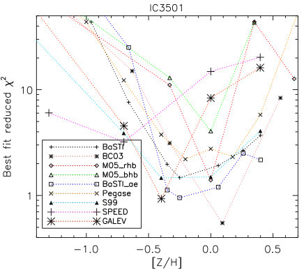
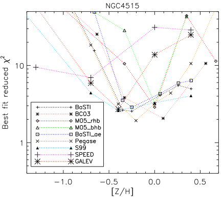
Figure 5: $\chi^{2}_{\nu}$ for best fitting age against [Z/H] for each model set, for IC3051 (top left), NGC4515 (top right), NGC4881 (bottom left) and NGC4874 (bottom right). Models are denoted by the symbols, and different metallicities connected by the line colours and styles, as denoted in the key in the box.

With the exception of the SPEED and Maraston models there is broad agreement between the models sets on [Z/H]. However the broad minima in the $\chi^{2}_{\nu}$ distributions illustrate further the significant uncertainties in estimates of [Z/H] or [Fe/H] from broad-band photometry.

6.3 Comparison with spectroscopic ages and metallicities

A useful comparison sample for the present work is provided by Trager et al. (2008), who present age, metallicity and [$\alpha$/Fe] estimates from spectroscopic line index measurements for a sample of 12 Coma cluster early-type galaxies, including 5 from our sample. However, it is important to note that the models used by Trager et al. (2008) are based on isochrones from Worthey (1994), unlike all of the models tested in this paper, so differences found may in part be due to the underlying stellar models. The quantitative effects on model predictions of line indices and spectral energy distributions due to changes in models are uncertain. Effects resulting from e.g. differing temperature and metallicity scales are being studied by Percival & Salaris (2009, in preparation).

In table  5 we reproduce the age and metallicity measurements from Table 5 of Trager et al. (2008). The quantities they tabulate are [Z/H] and [E/Fe], where E stands for Enhanced elements. [E/Fe] does not precisely correspond to [$\alpha$/Fe] in the BaSTI models, as the elements enhanced are somewhat different, as discussed by Trager et al. (2000a). However the key element for measuring [E/Fe] is Mg, which is an $\alpha$-element.

Table 5: Comparison with spectroscopic measurements from Trager et al. (2008)

	Trager et al.
	Age (Gyr)	$\sigma_{Age}$	[Z/H]	$\sigma_{[Z/H]}$	[E/Fe]	$\sigma_{[E/Fe]}$
NGC4867	3.0	0.3	0.54	0.04	0.20	0.01
NGC4872	4.8	0.4	0.36	0.02	0.18	0.01
NGC4871	4.5	0.4	0.36	0.04	0.14	0.01
NGC4873	4.5	0.4	0.32	0.04	0.19	0.01
NGC4874	7.9	1.0	0.38	0.04	0.17	0.01

Notes to Table 5: Where Trager et al. (2008) give asymmetric error bars, we quote here the larger value.

Trager et al. [Z/H] values are consistent with [Fe/H] as found from BaSTI and PÉGASE scaled solar models, and, using the relation [Z/H]=[Fe/H]+0.35 for the BaSTI $\alpha$-enhanced models, they are consistent with these also. BC03 do not have sufficient metallicity resolution for an adequate comparison. Trager et al. ages are older than the best fits for BaSTI and PÉGASE scaled solar models, but younger than those found for the $\alpha$-enhanced models. This might imply that models with [$\alpha$/Fe] $\sim$ +0.2 could provide both a better fit to the data and a better match to Trager et al. (2008), but this is impossible to test until such models are available.

Trager et al. (2008), and indeed much of the current work on stellar populations using spectroscopic data, uses the Lick index system. This is defined from fairly low resolution spectra ($\sim$8.4 Å FWHM), however for massive galaxies the effective resolution of the spectra is limited to this by the internal velocity dispersion ($\sigma\sim$ 200km/s). Ages measured on the Lick system have been shown to suffer from age-metallicity degeneracy, and also to be somewhat dependent upon which Balmer line index is used (e.g. Puzia et al. 2005; Brodie et al. 2005). Alternative index definitions have been proposed (Vazdekis & Arimoto 1999; Cervantes & Vazdekis 2009) which to some extent lift this degeneracy. In a future paper, we will compare the full, high-resolution BaSTI model spectra (Percival et al. 2009), with higher resolution spectra of lower velocity dispersion galaxies (e.g. Smith et al. 2009) to derive single or composite stellar population parameters.

6.4 Comparison with predictions from SBF magnitudes

Lee et al. (2009), using BaSTI isochrones, investigate predictions for the $I$-band Surface Brightness Fluctuation (SBF) magnitudes from scaled solar and $\alpha$-enhanced isochrones. Using data from Blakeslee et al. (2009), they find the $\alpha$-enhanced isochrones to be the better fit to the redder and more massive galaxies, whereas the scaled-solar models work better for bluer and less massive galaxies. They attribute this to the effect of oxygen enhancement on the upper RGB and AGB. In general this result agrees with what we see in our data, for instance in Table  3 we see that the $\alpha$-enhanced models provide lower values of $\chi^{2}$ for the most massive galaxies (this table is ordered by increasing luminosity). However there is still some work required to reconcile models, SBF magnitudes, and integrated colours, and indeed Lee et al. show that there are significant differences between Padova and BaSTI model predictions of ($V-I$) and $I$-band SBF magnitude, for the same scaled-solar abundances.

6.5 Effect of the IMF

In this study we have examined the effect of the choice of model set on the derived SSP parameters, however we have not examined different IMFs, having used the Kroupa (2001) IMF for all but one of our datasets, nor have we examined in detail the parametrisation of the treatment of the TP-AGB. Conroy et al. (2009) examined the effect of the TP-AGB and IMF using a dataset containing a much larger sample, but at lower photometric precision. It would be instructive to analyse our data with the Conroy et al. models, furthermore in a future paper we shall investigate, using the BaSTI models, the effect of different parametrisations of the IMF upon the derived colours.

7 Conclusions

We find that SSP models provide good fits to broad-band photometry from $u$ to $K_{s}$ bands, for a variety of morphologically early-type galaxies. Although we have tested only SSP models, we can at least say that the broad-band data do not require a more complicated star formation history. For galaxies brighter than $M_{V}\sim-20.5$ the best fits are usually provided by fully self-consistent $\alpha$-enhanced models, which are currently only available for BaSTI. This is consistent with a scenario in which the stars in massive galaxies formed over a relatively short time interval (Thomas et al. 2005). For galaxies fainter than $M_{V}\sim-20.5$ although the popular Bruzual & Charlot (2003) models provide in most cases objectively the best fit to the data, other scaled-solar abundance models including PÉGASE, GALEV, Starburst99 and BaSTI provide very similar solutions of very similar goodness of fit. This is consistent with formation of the stellar content of these galaxies over a longer time interval. We find that SPEED and Maraston (2005) models do not provide good fits to the data, and that the best fits they do provide occur at unrealistically low metal abundance and unrealistically young age respectively.

Broad-band photometry from $u$ to $K_{s}$, in the presence of realistic photometric errors, does not fully break the age-metallicity degeneracy, and the models which have sufficient metallicity resolution show that there are strongly anticorrelated uncertainties of $\simeq 0.25$ in log age, and $\simeq 0.18$ in log metallicity, on the derived population parameters. BaSTI $\alpha$-enhanced models fit at older ages than the scaled-solar models, but age-metallicity degeneracy is still present.

BaSTI models use stellar tracks with two values of both [$\alpha$/Fe] and the Reimers (1975) mass-loss parameter $\eta$, which controls horizontal branch morphology. We find that the latter has a much smaller effect than the former, but the range of this parameter that we have explored in this paper is small.

To improve our knowledge of stellar population parameters, it is important to investigate complementary techniques. These will include extending the wavelength range used further into the ultraviolet with HST/WFC3, which will provide an additional tool for breaking the age-metallicity degeneracy. However to utilize the UV photometry it is particularly important to understand the contribution of the regions of the HR diagram which contribute most to the UV flux, in particular the Horizontal Branch, Blue Stragglers, and any contribution from a young stellar component, for instance from merger induced star formation. Further complementary techniques include studies of the properties of star clusters associated with the galaxies, which sometimes show subpopulations indicating different stellar population parameters, and study of surface brightness fluctuations at near infra-red wavelengths, which are a powerful probe of the structure of the AGB and upper RGB.

References

- Adelman-McCarthy et al. (2008) Adelman-McCarthy, J.K. et al. 2008, ApJS, 175, 297
- Alongi et al. (1993) Alongi, M., Bertelli, G., Bressan, A., Chiosi, C., Fagotto, F., Greggio, L. & Nasi, E. 1993, A&AS, 97, 851
- Anders & Fritze-v. Alvensleben (2003) Anders, P. & Fritze-v. Alvensleben, U. 2003, A&A, 401, 1063
- Anders et al. (2004) Anders, P., Bissantz, N., Fritze-v. Alvensleben, U. & de Grijs, R. 2004, MNRAS, 347, 196
- Bell & de Jong (2000) Bell, E.F. & de Jong, R.S. 2000, MNRAS, 312, 497
- Blakeslee et al. (2009) Blakeslee, J.P. et al. 2009, ApJ, in press (arXiv:0901.1138)
- Bothun et al. (1984) Bothun, G.D., Romanishin, W., Strom, S.E. & Strom, K.M. 1984, AJ, 89, 1300
- Bothun & Gregg (1990) Bothun, G.D. & Gregg, M.D. 1990, ApJ, 350, 73
- Bressan et al. (1993) Bressan, A., Fagotto, F., Bertelli, G. & Chiosi, C. 1993, A&AS, 100, 647
- Brodie et al. (2005) Brodie, J.P., Strader, J., Denicoló, G., Beasley, M.A., Cenarro, A.J., Larsen, S.S. & Kuntschner, H. 2005, AJ, 129, 2643
- Bruzual & Charlot (1993) Bruzual, G. & Charlot, S. 1993, ApJ, 405, 538
- Bruzual & Charlot (2003) Bruzual, G. & Charlot, S. 2003, MNRAS, 344, 1000
- Burstein & Heiles (1982) Burstein, D. & Heiles, C. 1982, AJ, 87, 1165
- Busso et al. (2007) Busso, G., et al. 2007, A&A, 474, 105
- Cassisi et al. (1997a) Cassisi, S., Castellani, M. & Castellani, V. 1997a, A&A, 317, 108
- Cassisi et al. (1997b) Cassisi, S., degl’Innocenti, S. & Salaris, M. 1997b, MNRAS, 290, 515
- Cassisi et al. (2000) Cassisi, S., Castellani, V., Ciarcelluti, P., Piotto, G. & Zoccali, M. 2000, MNRAS, 315, 679
- Castelli & Kurucz (2003) Castelli, F. & Kurucz, R.L. 2003, in “Modelling of Stellar Atmospheres”, proceedings of the 210th symposium of the IAU, eds: N. Piskunov, W.W. Weiss, & D.F. Gray (ASP: San Francisco), pA20
- Cervantes & Vazdekis (2009) Cervantes, J.L. & Vazdekis, A. 2009, MNRAS, 392, 691
- Chabrier (2003) Chabrier, G. 2003, PASP, 115, 763
- Charlot & Bruzual (1991) Charlot, S. & Bruzual, G. 1991, ApJ, 367, 126
- Clayton & Cardelli (1988) Clayton, G.C. & Cardelli, J.A. 1988, AJ, 96, 695
- Cohen, Wheaton & Megeath (2003) Cohen, M., Wheaton, Wm. A., & Megeath, S.T., 2003, AJ, 126, 1090
- Conroy et al. (2009) Conroy, C., Gunn, J.E. & White, M. 2009, ApJ, submitted (arXiv:0809.4261)
- Cordier et al. (2007) Cordier, D., Pietrinferni, A., Cassisi, S., & Salaris, M. 2007, AJ, 133, 468
- Côté et al. (2004) Côté, P., et al. 2006, ApJS, 153, 223
- de Grijs et al. (005) de Grijs, R., Anders, P., Lamers, H.J.G.L.M., Bastian, N., Fritze-v. Alvensleben, U., Parmentier, G., Sharina, M.E. & Yi, S. 2005, MNRAS, 359, 874
- de Vaucouleurs et al. (1991) de Vaucouleurs, G., de Vaucouleurs, A., Corwin, H. G., Buta, R. J., Paturel, G., & Fouque, P. 1991, Third Reference Catalogue of Bright Galaxies (New York: Springer-Verlag)
- Eggleton (1971) Eggleton, P.P. 1971, MNRAS, 151, 351
- Eggleton (1972) Eggleton, P.P. 1972, MNRAS, 156, 361
- Eisenstein et al. (2006) Eisenstein, D.J. et al. 2006, ApJS, 167, 40.
- Eminian et al. (2008) Eminian, C., Kauffmann, G., Charlot, S., Wild, V., Bruzual, G., Rettura, A. & Loveday, J. 2008, MNRAS, 384, 930
- Fagotto et al. (1994a) Fagotto, F., Bressan, A., Bertelli, G. & Chiosi, C. 1994a, A&AS, 104, 365
- Fagotto et al. (1994b) Fagotto, F., Bressan, A., Bertelli, G. & Chiosi, C. 1994b, A&AS, 105, 29
- Fioc & Rocca-Volmerange (1997) Fioc, M. & Rocca-Volmerange, B. 1997, A&A, 326, 950
- Fioc & Rocca-Volmerange (1999) Fioc, M. & Rocca-Volmerange, B. 1999, arXiv:astro-ph/9912179
- Girardi et al. (1996) Girardi, L., Bressan, A., Chiosi, C., Bertelli, G. & Nasi, E. 1996, A&AS, 117, 113
- Girardi et al. (2000) Girardi, L., Bressan, A., Bertelli, G. & Chiosi, C. 2000, A&AS, 141, 371
- Groenewegen & de Jong (1993) Groenewegen, M.A.T. & de Jong, T. 1993, A&A, 267, 410
- Hempel & Kissler-Patig (2004a) Hempel, M. & Kissler-Patig, M. 2004a, A&A, 419, 863
- Hempel & Kissler-Patig (2004b) Hempel, M. & Kissler-Patig, M. 2004b, A&A, 428, 459
- Hempel et al. (2005) Hempel, M., Geisler, D. Hoard, D.W. & Harris, W.E. 2005, A&A, 439, 59
- James et al. (2006) James, P.A., Salaris, M., Davies, J.I., Phillipps, S. & Cassisi, S. 2006, MNRAS, 367, 339
- Jimenez et al. (1995) Jimenez, R., Jorgensen, U.G., Thejll, P. & Macdonald, J. 1995, MNRAS, 275, 1245
- Jimenez et al. (1996) Jimenez, R., Thejll, P., Jorgensen, U.G., Macdonald, J. & Pagel, B. 1996, MNRAS, 282, 926
- Jimenez et al. (2004) Jimenez, R., Macdonald, J., Dunlop, J., Padoan, P. & Peacock, J.A. 2004, MNRAS, 349, 240
- Jorgensen (1991) Jorgensen, U.G. 1991, A&A, 246, 118
- Kaviraj et al. (2007a) Kaviraj, S., Rey, S.-C., Rich, R.M., Yoon, S.-J. & Yi, S.K. 2007a, MNRAS, 381, L74
- Kaviraj et al. (2007b) Kaviraj, S. et al. 2007b, ApJS, 173, 619
- Kim & Lee (2007) Kim, S.S. & Lee, M.G. 2007, PASP, 119, 1449
- Kodama & Arimoto (1997) Kodama, T. & Arimoto, N. 1997, A&A, 320, 41
- Koleva et al. (2008) Koleva, M., Prugniel, Ph., Ocvirk, P., Le Borgne, D. & Soubiran, C. 2008, MNRAS, 385, 1998
- Kroupa (2001) Kroupa, P. 2001, MNRAS, 322, 231
- Kundu et al. (2005) Kundu, A. et al. 2005, ApJL, 634, L41
- Kuntschner et al. (2001) Kuntschner, H., Lucey, J.R., Smith, R.J., Hudson, M.J. & Davies, R.L. 2001, MNRAS, 323, 615
- Kurucz (1993) Kurucz, R.L. 1993, “ATLAS9 Stellar Atmosphere Programs and 2 km/s grid, Smithsonian Astrophysical Observatory.”, CD-ROM No. 13
- Lançon & Mouhcine (2002) Lançon, A. & Mouhcine, M. 2002, A&A, 393, 167
- Le Borgne et al. (2003) Le Borgne, J.-F. et al. 2003, A&A, 402, 433
- Lee et al. (2007) Lee, H.-C., Worthey, G., Trager, S.C. & Faber, S.M. 2007, ApJ, 664, 215
- Lee et al. (2009) Lee, H.-C., Worthey, G. & Blakeslee, J.P., ApJ, in press (arXiv:0902.1177)
- Lejeune (1997) Lejeune, T., Cuisinier, F & Buser, R. 1997, A&AS, 125, 229
- Lejeune (1998) Lejeune, T., Cuisinier, F & Buser, R. 1998, A&AS, 130, 65
- Maraston (1998) Maraston, C. 1998, MNRAS, 300, 872
- Maraston (2005) Maraston, C. 2005, MNRAS, 362, 799
- Maraston et al. (2008) Maraston, C., Strömbäck, G., Thomas, D., Wake, D.A. & Nichol, R.C. 2008, ApJL, submitted (arXiv:0809.1867v1)
- Marigo & Girardi (2007) Marigo, P. & Girardi, L. 2007, A&A, 469, 239
- Michard (2005) Michard, R. 2005, A&A, 429, 819
- Nelan et al. (2005) Nelan, J.E., Smith, R.J., Hudson, M.J., Wegner, G.A., Lucey, J.R., Moore, S.A.W., Quinney, S.J. & Suntzeff, N.B. 2005, ApJ, 632, 137.
- Ocvirk et al. (2006a) Ocvirk, P., Pichon, C., Lançon, A. & Thiébaut, E. 2006a, MNRAS, 365, 46
- Ocvirk et al. (2006b) Ocvirk, P., Pichon, C., Lançon, A. & Thiébaut, E. 2006b, MNRAS, 365, 74
- Padmanabhan et al. (2008) Padmanabhan, N. et al. 2008, ApJ, 674, 1217
- Panter et al. (2003) Panter, B., Heavens, A.F. & Jimenez, R. 2003, MNRAS, 343, 1145
- Panter et al. (2007) Panter, B., Jimenez, R., Heavens, A.F. & Charlot, S. 2007, MNRAS, 378, 1550
- Peletier & Balcells (1996) Peletier, R.F. & Balcells, M. 1996, AJ, 111, 2238
- Peletier et al. (1990) Peletier, R.F., Valentijn, E.A. & Jameson, R.F. 1990, A&A, 233, 62
- Percival et al. (2008) Percival, S.M., Salaris, M., Cassisi, S. & Pietrinferni, A. 2008, ApJ, 690, 427
- Pessev et al. (2008) Pessev, P.M., Goudfrooij, P., Puzia, T.H. & Chandar, R. 2008, MNRAS, 385, 1535
- Pickles (1998) Pickles, A.J. 1998, PASP, 110, 863
- Pietrinferni et al. (2004) Pietrinferni, A., Cassisi, S., Salaris, M. & Castelli, F. 2004, ApJ, 612, 168
- Pietrinferni et al. (2006) Pietrinferni, A., Cassisi, S., Salaris, M. & Castelli, F. 2006, ApJ, 642, 797
- Poggianti et al. (2001a) Poggianti, B.M. et al. 2001a, ApJ, 562, 689
- Poggianti et al. (2001b) Poggianti, B.M. et al. 2001b, ApJ, 563, 118
- Puzia et al. (2002) Puzia, T.H., Zepf, S.E., Kissler-Patig, M., Hilker, M., Minniti, D. & Goudfrooij, P. 2002, A&A, 391, 453
- Puzia et al. (2005) Puzia, T.H., Kissler-Patig, M., Thomas, D., Maraston, C., Saglia, R.P., Bender, R., Goudfrooij, P. & Hempel, M. 2005, A&A, 439, 997
- Rakos et al. (2007) Rakos, K., Schombert, J. & Odell, A. 2007, ApJ, 658, 929
- Rakos et al. (2008) Rakos, K., Schombert, J. & Odell, A. 2008, ApJ, 677, 1019
- Rawle et al. (2008) Rawle, T.D., Smith, R.J., Lucey, J.R., Hudson, M.J. & Wegner, G.A. 2008, MNRAS, 385, 2097
- Reimers (1975) Reimers, D. 1975, Mem. Soc. R. Sci. Liège, 6, 369
- Renzini & Buzzoni (1986) Renzini, A. & Buzzoni, A. 1986, in “Spectral evolution of galaxies”, eds: G. Chiosi & A. Renzini (D. Reidel: Dordrecht), p195
- Sánchez-Blázquez et al. (2006) Sánchez-Blázquez, P., Gorgas, J., Cardiel, N. & González, J.J. 2006, A&A, 457, 809
- Schlegel et al. (1998) Schlegel, D.J., Finkbeiner, D.P. & Davis, M. 1998, ApJ, 500, 525
- Schulz et al. (2002) Schulz, J., Fritze-v. Alvensleben, U., Möller, C.S. & Fricke, K.J. 2002, A&A, 392, 1
- Smith et al. (2009) Smith, R.J., Lucey, J.R., Hudson, M.J., Allanson, S.P., Bridges, T.J., Hornschemeier, A.E., Marzke, R.O. & Miller, N.A. 2009, MNRAS, 392, 1265
- Skrutskie et al. (2006) Skrutskie, M.F. et al. 2006, AJ, 131, 1163
- Thomas et al. (2005) Thomas, D., Maraston, C., Bender, R. & Mendes de Oliveira, C. 2005, ApJ, 621, 673.
- Tojeiro et al. (2007) Tojeiro, R., Heavens, A.F., Jimenez, R. & Panter, B. 2007, MNRAS, 381, 1252
- Trager et al. (2000a) Trager, S.C., Faber, S.M., Worthey, G, González, J.J. 2000a, AJ 119, 1645.
- Trager et al. (2000b) Trager, S.C., Faber, S.M., Worthey, G, González, J.J. 2000b, AJ 120, 165.
- Trager et al. (2008) Trager, S.C., Faber, S.M. & Dressler, A. 2008, MNRAS, 386, 715
- Vassiliadis & Wood (1993) Vassiliadis, E. & Wood, P.R. 1993, ApJ, 413, 641
- Vassiliadis & Wood (1994) Vassiliadis, E. & Wood, P.R. 1994, ApJS, 92, 125
- Vazdekis & Arimoto (1999) Vazdekis, A. & Arimoto, N. 1999, ApJ, 525, 144
- Vázquez & Leitherer (2005) Vázquez, G.A. & Leitherer, C. 2005, ApJ, 621, 695
- Westera et al. (2002) Westera, P., Lejeune, T., Buser, R., Cuisinier, F. & Bruzual, G. 2002, A&A, 381, 524
- (105) Worthey, G. 1994, ApJS, 95, 107