Synthesis of linear quantum stochastic systems via quantum feedback networks

Abstract

Recent theoretical and experimental investigations of coherent feedback control, the feedback control of a quantum system with another quantum system, has raised the important problem of how to synthesize a class of quantum systems, called the class of linear quantum stochastic systems, from basic quantum optical components and devices in a systematic way. The synthesis theory sought in this case can be naturally viewed as a quantum analogue of linear electrical network synthesis theory and as such has potential for applications beyond the realization of coherent feedback controllers. In earlier work, Nurdin, James and Doherty have established that an arbitrary linear quantum stochastic system can be realized as a cascade connection of simpler one degree of freedom quantum harmonic oscillators, together with a direct interaction Hamiltonian which is bilinear in the canonical operators of the oscillators. However, from an experimental perspective and based on current methods and technologies, direct interaction Hamiltonians are challenging to implement for systems with more than just a few degrees of freedom. In order to facilitate more tractable physical realizations of these systems, this paper develops a new synthesis algorithm for linear quantum stochastic systems that relies solely on field-mediated interactions, including in implementation of the direct interaction Hamiltonian. Explicit synthesis examples are provided to illustrate the realization of two degrees of freedom linear quantum stochastic systems using the new algorithm.

1 Introduction

Linear quantum stochastic systems (see, e.g., [1, 2, 3, 4]) arise as an important class of models in quantum optics [5] and in phenomenological models of quantum RLC circuits [6]. They are used, for instance, to model optical cavities driven by coherent laser sources and are of interest for applications in quantum information science. In particular, they have the potential as a platform for realization of entanglement networks [7, 8, 9] and to function as sub-sytems of a continuous variable quantum information system (e.g., the scheme of [10]). Recently, there has also been interest in the possibilities of control of linear quantum stochastic systems with a controller which is a quantum system of the same type [11, 2, 3, 12] (thus involving no measurements of quantum signals), often referred to as “coherent-feedback control”, and an experimental realization of a coherent-feedback control system for broadband disturbance attenuation has been successfully demonstrated by Mabuchi [12]. Linear quantum stochastic systems are a particularly attractive class of quantum systems to study for coherent control because of their simple structure and complete parametrization by a number of matrix parameters.

A natural and important question that arose out of the studies on coherent control is how an arbitrary linear quantum stochastic system can be built or synthesized in a systematic way, in the quantum optical domain, from a bin of quantum optical components like beam splitters, phase shifters, optical cavities, squeezers, etc; this can be viewed as being analogous to the question in electrical network synthesis theory of how to synthesize linear analog circuits from basic electrical components like resistors, capacitors, inductors, op-amps, etc. The synthesis problem is not only of interest for quantum control, but is a timely subject in its own right given the current intense research efforts in quantum information science (see, e.g., [13]). These developments present significant opportunities for investigations of a network synthesis theory (e.g., [14] for linear electrical networks) in the quantum domain as a significant direction for future development of circuit and systems theory. In particular, such a quantum synthesis theory may be especially relevant for the theoretical foundations, development and design of future linear photonic integrated circuits.

As a first step in addressing the quantum synthesis question, Nurdin, James and Doherty [4] have shown that any linear quantum stochastic system can, in principle, be synthesized by a cascade of simpler one degree of freedom quantum harmonic oscillators together with a direct interaction Hamiltonian between the canonical operators of these oscillators. Then they also showed how these one degree of freedom harmonic oscillators and direct bilinear interaction Hamiltonian can be synthesized from various quantum optical components. However, from an experimental point of view, direct bilinear interaction Hamiltonians between independent harmonic oscillators are challenging to implement experimentally with current technology for systems that have more than just a few degrees of freedom (possibly requiring some complex spatial arrangement and orientation of the oscillators) and therefore it becomes important to investigate approximate methods for implementing this kind of interaction. Here we propose such a method by exploiting the recent theory of quantum feedback networks [15]. In our scheme, the direct interaction Hamiltonians are approximately realized by appropriate field interconnections among oscillators. The approximation is based on the assumption that the time delays required in establishing field interconnections are vanishingly small, which is typically the case in quantum optical systems where quantum fields propagate at the speed of light.

The paper is organized as follows. Section 2 provides a brief overview of linear quantum stochastic systems and the concatenation and series product of such sytems. Section 3 recalls the notion of a model matrix and the concatenation of model matrices, while Section 4 recalls the notion of edges, their elimination, and reduced Markov models. Section 5 reviews a prior synthesis result from [4]. Section 6 presents the main results of this paper and an example to illustrate their application to the realization of a two degrees of freedom linear quantum stochastic system. In Section 7 the special class of passive linear quantum stochastic systems is introduced and it is shown that such systems can be synthesized by using only passive sub-systems and components. Another synthesis example for a passive system is also presented. Finally, Section 8 offers the conclusions of this paper. In order to focus on the results, all proofs are collected together in the Appendix.

2 Linear quantum stochastic systems

This section serves to recall some notions and results on linear quantum stochastic systems that are pertinent for the present paper. A relatively detailed overview of linear quantum stochastic systems can be found in [4] and further discussions in [1, 2, 16, 3], thus they will not be repeated here.

Throughout the paper we shall use the following notations: $i=\sqrt{-1}$, ^∗ will denote the adjoint of a linear operator as well as the conjugate of a complex number, if $A=[a_{jk}]$ is a matrix of linear operators or complex numbers then $A^{\#}=[a_{jk}^{*}]$, and $A^{{\dagger}}$ is defined as $A^{{\dagger}}=(A^{\#})^{T}$, where ^T denotes matrix transposition. We also define, $\Re\{A\}=(A+A^{\#})/2$ and $\Im\{A\}=(A-A^{\#})/2i$ and denote the identity matrix by $I$ whenever its size can be inferred from context and use $I_{n}$ to denote an $n\times n$ identity matrix. Similarly, $0$ denotes a matrix with zero entries whose dimensions can be determined from context, while $0_{m\times n}$ denotes a matrix with specified dimension $m\times n$ with zero entries. Other useful notations that we shall employ is ${\rm diag}(M_{1},M_{2},\ldots,M_{n})$ (with $M_{1},M_{2},\ldots,M_{n}$ square matrices) to denote a block diagonal matrix with $M_{1},M_{2},\ldots,M_{n}$ on its diagonal block, and ${\rm diag}_{n}(M)$ ($M$ a square matrix) denotes a block diagonal matrix with the matrix $M$ appearing on its diagonal blocks $n$ times.

Let $q_{1},p_{1},q_{2},p_{2},\ldots,q_{n},p_{n}$ be the canonical position and momentum operators of a many degrees of freedom quantum harmonic oscillator satisfying the canonical commutation relations (CCR) $[q_{j},p_{k}]=2i\delta_{jk}$. The integer $n$ will be referred to as the degrees of freedom of the oscillator. Letting $x=(q_{1},p_{1},q_{2},p_{2},\ldots,q_{n},p_{n})^{T}$ then these commutation relations can be written compactly as:

$$xx^{T}-(xx^{T})^{T}=2i\Theta,$$

with $\Theta={\rm diag}_{n/2}(J)$ and $J=\left[\begin{array}[]{cc}0&1\\ -1&0\end{array}\right]$. Here a linear quantum stochastic system $G$ is a quantum system defined by three parameters: (i) A quadratic Hamiltonian $H=\frac{1}{2}x^{T}Rx$ with $R=R^{T}\in\mathbb{R}^{n\times n}$, (ii) a coupling operator $L=Kx$ where $K$ is an $m\times n$ complex matrix and (iii) a unitary $m\times m$ scattering matrix $S$. We also assume that the system oscillator is in an initial state with density operator $\rho$. For shorthand, we write $G=(S,L,H)$ or $G=(S,Kx,\frac{1}{2}x^{T}Rx)$. The time evolution, in the interaction picture, $X(t)$ of $x$ ($t\geq 0$) is given by the quantum stochastic differential equation (QSDE):

$$dX(t) =AX(t)dt+B\left[\begin{array}[]{c}dA(t)\\ dA(t)^{\#}\end{array}\right];\,X(0)=x.$$ (3)

$$dY(t) =CX(t)dt+DdA(t),$$ (4)

with

$$A =2\Theta(R+\Im\{K^{{\dagger}}K\});\;B=2i\Theta[\begin{array}[]{cc}-K^{{\dagger}}S&K^{T}S^{\#}\end{array}];\;$$

$$C =K;\;D=S,$$

where $A(t)=(A_{1}(t),\ldots,A_{n}(t))^{T}$ is a vector of input vacuum bosonic noise fields and $Y(t)=(Y_{1}(t),\ldots,Y_{n}(t))^{T}$ is a vector of output fields that results from the interaction of $A(t)$ with the harmonic oscillator. Note that the dynamics of $X(t)$ and $Y(t)$ are linear. We refer to $(A,B,C,D)$ as the system matrices of $G$. For the case when $n=1$, we shall often refer to the linear quantum stochastic system as a one degree of freedom (open quantum harmonic) oscillator.

Elements of $A(t)$ and $Y(t)$ may be partitioned into blocks. For example, $A(t)$ may be partitioned as $A(t)=(A_{r_{1}}(t)^{T},\ldots,A_{r_{n_{\rm in}}}(t)^{T})$ and $Y(t)$ as $Y(t)=(Y_{s_{1}}(t)^{T},\ldots,Y_{s_{n_{\rm out}}}(t)^{T})^{T}$, where $A_{r_{j}}(t)$ and $Y_{s_{k}}(t)$ are vectors of bosonic input and output field operators of length $n_{r_{j}}$ and $n_{s_{k}}$, respectively, such that $\sum_{j=1}^{n_{\rm in}}n_{r_{j}}=\sum_{k=1}^{n_{\rm out}}n_{s_{k}}=m$. We refer to $n_{r_{j}}$ and $n_{s_{k}}$ as the multiplicity of $A_{r_{j}}(t)$ and $Y_{s_{k}}(t)$, respectively. It is important to keep in mind that the sum of the multiplicities of all input and output partitions sum up to $m$, the total number of all input and output fields. With this partitioning, a linear quantum stochastic system $G$ may be viewed as a quantum device having $n_{\rm in}$ input ports and $n_{\rm out}$ output ports as illustrated in Figure 1. The multiplicity of a port is then defined as the multiplicity of the input or output fields coming into or going out of that port.

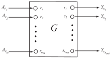
Figure 1: A linear quantum stochastic system viewed as a device with $n_{\rm in}$ input ports and $n_{\rm out}$ output ports.

Let us also recall the notion of the concatenation ($\boxplus$) and series products ($\triangleleft$) between open quantum systems developed in [17]. The concatenation product $G_{1}\boxplus G_{2}$ between $G_{1}=(S_{1},L_{1},H_{1})$ and $G_{2}=(S_{2},L_{2},H_{2})$ defines another quantum linear system given by:

$$G_{1}\boxplus G_{2}=({\rm diag}(S_{1},S_{2}),[\begin{array}[]{cc}L_{1}^{T}&L_{2}^{T}\end{array}]^{T},H_{1}+H_{2}),$$

while if $G_{1}$ and $G_{2}$ have the same number of input (and output) fields the series product $G_{2}\triangleleft G_{1}$ defines another linear quantum system given by:

$$G_{2}\triangleleft G_{1}=(S_{2}S_{1},L_{2}+S_{2}L_{1},H_{1}+H_{2}+\Im\{L_{2}^{{\dagger}}S_{2}L_{1}\}).$$

Note that in the definition of the concatenation and series product, it is not required that the elements of $L_{1}$ and $L_{2}$ and of $H_{1}$ and $H_{2}$ are commuting. That is, $G_{1}$ and $G_{2}$ may possibly be sub-components of the same system. Also both operations are associative, but neither operations are commutative. By the associativity, the operations $\boxplus_{j=1}^{n}G_{j}=G_{1}\boxplus G_{2}\boxplus\ldots\boxplus G_{n}$ and $G_{n}\triangleleft\ldots\triangleleft G_{2}\triangleleft G_{1}$ are unambiguously defined.

The concatenation product corresponds to collecting together the parameters of $G_{1}$ and $G_{2}$ to form one larger concatenated system, and the series product is a mathematical abstraction of the physical operation of cascading $G_{1}$ onto $G_{2}$, that is, passing the output fields of $G_{1}$ as the input fields to $G_{2}$. The cascaded system is then another linear quantum stochastic system with parameters given by the series product formula.

3 The model matrix and concatenation of model matrices

The system $G=(S,L,H)$ can also be represented using a so-called model matrix [15]. This representation will be particularly useful for the goals of the present paper. For $G$ the model matrix representation $M(G)$ is given by (the partitioned matrix):

$$M(G)=\left[\begin{array}[]{cccc}-iH-\frac{1}{2}L^{{\dagger}}L&-L^{{\dagger}}S\\ L&S\end{array}\right],$$ (5)

with the understanding that if $L$ is partitioned as $L=(L_{1}^{T},L_{2}^{T},\ldots,L_{n_{\rm out}}^{T})^{T}$ with $L_{j}\in m_{j}\times 2$ and $\sum_{j=1}^{n_{\rm out}}m_{j}=m$ and $S$ is partitioned accordingly as $S=[S_{jk}]_{j=1,\ldots,n_{\rm out},k=1,\ldots,n_{\rm in}}$ with $S_{jk}\in\mathbb{C}^{m_{j}\times m^{\prime}_{k}}$ and $\sum_{k=1}^{n_{\rm in}}m^{\prime}_{k}=m$, then the model matrix above can be expressed with respect to this partition as:

$$M(G)=\left[\begin{array}[]{cccc}-iH-\frac{1}{2}\sum_{j=1}^{n_{\rm out}}L_{j}^{{\dagger}}L_{j}&-\sum_{j=1}^{n_{\rm out}}L_{j}^{{\dagger}}S_{j1}&\ldots&-\sum_{j=1}^{n_{\rm out}}L_{j}^{{\dagger}}S_{jn_{\rm in}}\\ L_{1}&S_{11}&\ldots&S_{1n_{\rm in}}\\ \vdots&\vdots&\ddots&\vdots\\ L_{n_{\rm out}}&S_{n_{\rm out}1}&\ldots&S_{n_{\rm out}n_{\rm in}}\end{array}\right].$$ (10)

Also, with respect to a particular partitioning of $M(G)$, it is convenient to attach a unique label to each row and column of the partition. For example, for the partitioning (10) we may give the labels $s_{0},s_{1},\ldots,s_{n_{\rm out}}$ for the first, second, …, $n_{\rm out}+1$-th row of $M(G)$, respectively, and $r_{0},r_{1},\ldots,r_{n_{\rm in}}$ for the first, second, …, $n_{\rm in}+1$-th column of $M(G)$, respectively. Moreover, with respect to this labelling (and analogously for any other labelling scheme chosen), elements of the blocks are denoted as:

$$M_{s_{0}r_{0}}(G) =-iH-\frac{1}{2}\sum_{j=1}^{n_{\rm out}}L_{j}^{{\dagger}}L_{j};\;M_{s_{0}r_{k}}(G)=-\sum_{j=1}^{n_{\rm out}}L_{j}^{{\dagger}}S_{jk},\,k>0;$$

$$M_{s_{j}r_{0}}(G) =L_{j},\,j>0;\;M_{s_{j}r_{k}}=S_{jk},\,j,k>0.$$

Since $M(G)$ is another representation of a physical system described by $G$, and $G$ can be identified directly from the entries of $M(G)$, we will often omit the $G$ and for brevity write a model matrix simply as $M$ and denote its entries by $M_{\alpha\beta}$, with $\alpha$ ranging over row labels and $\beta$ ranging over the column labels. Thus, we also refer to the triple $S,L,H$ in (5) as parameters of the model matrix $M$.

Several model matrices can be concatenated to form a larger model matrix. Such a concatenation corresponds to collecting together the model parameters of the individual matrices in a larger model matrix and is again denoted by the symbol $\boxplus$. If $G_{1}=(S_{1},L_{1},H_{1})$ and $G_{2}=(S_{2},L_{2},H_{2})$ then the concatenation $M(G_{1})\boxplus M(G_{2})$ is defined as:

$$M(G_{1})\boxplus M(G_{2}) =\left[\begin{array}[]{ccc}-iH_{1}-iH_{2}-\frac{1}{2}L_{1}^{{\dagger}}L_{1}-\frac{1}{2}L_{2}^{{\dagger}}L_{2}&-L_{1}^{{\dagger}}S_{1}&-L_{2}^{{\dagger}}S_{2}\\ L_{1}&S_{1}&0\\ L_{2}&0&S_{2}\end{array}\right]$$

$$=M(G_{1}\boxplus G_{2}).$$

4 Edges, Elimination of Edges, and Reduced Markov Models

Following [15], a particular row partition labelled $s_{k}$ with $k>0$ in a model matrix can be associated with an output port $s_{k}$ (having multiplicity $n_{s_{k}}$) while a particular column partition $r_{j}$ with $j>0$ can be associated with an input port $r_{j}$ (having multiplicity $n_{r_{j}}$). In a system which is the concatenation of several sub-systems, it is possible to connect an output port $s_{k}$ from one sub-system to an input port $r_{j}$ of another sub-system (possibly the same sub-system to which the output port belongs) to form what is called an internal edge denoted by $(s_{k},r_{j})$. For this connection to be possible, the ports $s_{k}$ and $r_{j}$ must have the same multiplicity. Such an edge then represents a channel from port $s_{k}$ to port $r_{j}$. All ports which are connected to other ports to form an internal edge or channel are referred to as internal ports and fields coming into or leaving such ports are called internal fields. All other input and output ports that are not connected in this way are viewed as having semi-infinite edges (since they do not terminate at some input or output port, as appropriate) and are referred to as external ports and the associated semi-infinite edges are referred to as external edges. Fields coming into or leaving external ports are called external fields. From a point of view in line with circuit theory, one may think of a linear quantum stochastic system as being a “node” on a network and quantum fields as quantum “wires” that can connect different nodes.

In any internal edge $(s_{k},r_{j})$, there is a finite delay present due to the time which is required for the signal from port $s_{k}$ to travel to port $r_{j}$. As a consequence of these finite time delays, concatenated systems with internal edges cannot be represented by a Markov model such as presented in Section 2 (see [4] and the references therein for an overview of Markov models). However, as shown in [15], the non-Markov model converges to a reduced Markov model in the limit that the time delay on all internal edges go to zero. That is, for negligibly small time delays, the reduced Markov model acts as an approximation of the non-Markov model. In particular, such a reduced model serves as a powerful approximation of quantum optical networks in which signals travel at the speed of light and the time delay can be considered to be practically zero if the internal input and output ports are not extremely far apart. We recall the following results:

Theorem 1

[15, Theorem 12 and Lemma 16] Let $\tau_{(s_{k},r_{j})}$, $j,k>0$, be the time delay for an internal edge $(s_{k},r_{j})$ and assume that $I-S_{kj}$ is invertible. Then in the limit that $\tau_{(s_{k},r_{j})}\downarrow 0$, $M(G)$ with the edge $(s_{k},r_{j})$ connected reduces to a simplified model matrix $M_{\rm red}$ with input ports labelled $r_{0},r_{1},\ldots,r_{j-1},r_{j+1},\ldots,r_{n_{\rm out}}$ and output ports labelled $s_{0},s_{1},\ldots,s_{k-1},s_{k+1},\ldots,s_{n_{\rm in}}$ (i.e., the connected ports $r_{j}$ and $s_{k}$ are removed from the labelling and the associated row and column removed from $M(G)$). The block entries of $M_{\rm red}$ are given by:

$$(M_{\rm red})_{\alpha\beta}=M_{\alpha\beta}+M_{\alpha r_{j}}(1-S_{kj})^{-1}M_{s_{k}\beta},$$

with $\alpha\in\{s_{0},s_{1},\ldots,s_{n_{\rm out}}\}\backslash\{s_{k}\}$ and $\beta\in\{r_{0},r_{1},\ldots,r_{n_{\rm in}}\}\backslash\{r_{j}\}$. $M_{\rm red}$ is the model matrix of a linear quantum stochastic system $G_{\rm red}$ with parameters:

$$(S_{\rm red})_{pq} =S_{pq}+S_{pj}(I-S_{kj})^{-1}S_{kq}$$

$$(L_{\rm red})_{p} =L_{p}+S_{pj}(I-S_{kj})^{-1}L_{k}$$

$$H_{\rm red} =H+\sum_{p=1}^{n_{\rm out}}\Im\{L_{p}^{{\dagger}}S_{pj}(I-S_{kj})^{-1}L_{p}\},$$

for all $p\in\{1,2,\ldots,n_{\rm out}\}\backslash\{k\}$ and $q\in\{1,2,\ldots,n_{\rm in}\}\backslash\{j\}$.

Several internal edges may be eliminated one at a time in a sequence leading to a corresponding sequence of reduced model matrices. The following result shows that such a procedure is unambiguous:

Theorem 2

[15, Lemma 17] The reduced model matrix obtained after eliminating all the internal edges in a set of internal edges one at a time is independent of the sequence in which these edges are eliminated.

Suppose that $M$ can be partitioned as:

$$\left[\begin{array}[]{ccc}-iH-1/2L_{\rm i}^{{\dagger}}L_{\rm i}-1/2L_{\rm e}^{{\dagger}}L_{\rm e}&-L_{\rm i}^{{\dagger}}S_{\rm ii}-L_{\rm i}^{{\dagger}}S_{\rm ei}&-L_{\rm e}^{{\dagger}}S_{\rm ie}-L_{\rm i}^{{\dagger}}S_{\rm ii}\\ L_{\rm i}&S_{\rm ii}&S_{\rm ie}\\ L_{\rm e}&S_{\rm ei}&S_{\rm ee}\end{array}\right],$$ (14)

where the subscript ${\rm i}$ refers to “internal” and ${\rm e}$ to “external”. That is, parameters with subscript ${\rm i}$ or ${\rm ii}$ pertain to internal ports, those with subscript ${\rm e}$ or ${\rm ee}$ pertain to external ports, while $S_{\rm ie}$ and $S_{\rm ei}$ pertain to scattering of internal fields to external fields and vice-versa, respectively. Interconnection among internal input and output ports can then be conveniently encoded by a so-called adjacency matrix. Let $n_{\rm i}$ denote the total multiplicity of internal input and output ports and let us view a port with multiplicity $k$ as $k$ distinct ports of multiplicity $1$. Suppose that these multiplicity 1 ports are numbered consecutively starting from 1, then an adjacency matrix $\eta$ is an $n_{\rm i}\times n_{\rm i}$ square matrix whose entries are either $1$ or $0$ with $\eta(j,k)=1$ ($j,k\in\{1,2,\ldots,n_{\rm i}\})$ only if the $j$-th output port and the $k$-th input port form a channel or internal edge. Note that at most only a single element in any row or column of $\eta$ can take the value 1. Internal edges can be simultaneously eliminated as follows:

Theorem 3

[15, Section 5] Suppose that $M$ has a partitioning based on internal and external components as in (14) and that connections between internal ports have been encoded in an adjacency matrix $\eta$. If $(\eta-S_{\rm ii})^{-1}$ exists, then the reduced model matrix $M_{\rm red}$ after simultaneous elimination of all internal edges has the parameters:

$$S_{\rm red} =S_{\rm ee}+S_{\rm ei}(\eta-S_{\rm ii})^{-1}S_{\rm ie}$$

$$L_{\rm red} =L_{\rm e}+S_{\rm ei}(\eta-S_{\rm ii})^{-1}L_{\rm i}$$

$$H_{\rm red} =H+\sum_{j={\rm i,e}}\Im\{L_{j}^{{\dagger}}S_{j{\rm i}}(\eta-S_{\rm ii})^{-1}L_{\rm i}\}.$$

5 Prior work

Let $G=(I_{m},Kx,\frac{1}{2}x^{T}Rx)$ be a linear quantum stochastic system with $K=[\begin{array}[]{ccc}K_{1}&\ldots&K_{n}\end{array}]\in\mathbb{C}^{m\times 2n}$ and $R=[R_{jk}]_{j,k=1,\ldots,n}\in\mathbb{R}^{2n\times 2n}$ ($R_{kj}=R_{jk}^{T}$). Let $x_{j}=(q_{j},p_{j})^{T}$ so that $x=(x_{1}^{T},\ldots,x_{n}^{T})^{T}$ and $x$ satisfies the commutation relations of Section 2. Then the following result holds:

Theorem 4

[4] Let $G_{k}=(I,K_{k}x_{k},\frac{1}{2}x_{k}^{T}R_{kk}x_{k})$. Then

$$G=(0,0,H^{d})\boxplus(G_{n}\triangleleft\ldots\triangleleft G_{2}\triangleleft G_{1}),$$

where $H^{d}=\sum_{j=1}^{n-1}\sum_{k=j+1}^{n}H^{d}_{jk}$ and $H^{d}_{jk}=x_{k}^{T}(R_{jk}^{T}-\Im\{K_{k}^{{\dagger}}K_{j}\})x_{j}$.

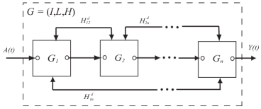
Figure 2: Realization of $G=(I,L,H)$ via a cascade connection of one degree of freedom quantum harmonic oscillators $G_{j}$ and bilinear direct interaction Hamiltonians $H_{jk}$ between every pair of oscillators

The theorem says that $G$ can in principle be constructed as the cascade connection $G_{n}\triangleleft\ldots\triangleleft G_{2}\triangleleft G_{1}$ of the one degree of freedom oscillators $G_{1},G_{2},\ldots,G_{n}$, together with a direct bilinear interaction Hamiltonian $H^{d}$ which is the sum of bilinear interaction Hamiltonians $H^{d}_{jk}$ between each pair of oscillator $G_{j}$ and $G_{k}$. This construction is depicted in Figure 2. It was then shown how each $G_{k}$ can be constructed from certain basic quantum optical components and how $H^{d}_{jk}$ can be implemented between any pair of oscillators. However, a drawback of this approach, based on what is feasible with current technology, is the challenging nature of implementing $H^{d}$. This may possibly involve complex positioning and orientation of the oscillators and thus practically challenging for systems with more than just a few degrees of freedom. Although advances in experimental methods and emergence of new technologies may eventually alleviate this difficulty, it is naturally of immediate interest to also explore alternative methods of implementing this interaction Hamiltonian, at least approximately. In the next section, we propose such an alternative synthesis by exploiting the theory of quantum feedback networks that has been elaborated upon in preceding sections of the paper.

6 Main synthesis results

For $j=1,\ldots,n$, let $G_{jk}=(S_{jk},L_{jk},0)$ for $k=1,\ldots,n,k\neq j$, and $G_{jj}=(S_{jj},L_{j},H_{j})$, with $S_{jk}\in\mathbb{C}^{c_{jk}\times c_{jk}}$, $c_{jk}=c_{kj}$ and $c_{jj}=m$, $L_{jk}=K_{jk}x_{j}$, and $H_{j}=\frac{1}{2}x_{j}^{T}R_{j}x_{j}$ with $R_{j}=R_{j}^{T}\in\mathbb{R}^{2\times 2}$. Here $x_{j}=(q_{j},p_{j})^{T}$ is as defined in the previous section. Let $G_{j}=\boxplus_{k=1}^{n}G_{jk}$ for $j=1,\ldots,n$, and note that $G_{j}=(S_{j},L_{j},H_{j})$ with $S_{j}={\rm diag}(S_{j1},S_{j2},\ldots,S_{jn})$, $L_{j}=(L_{j1}^{T},L_{j2}^{T},\ldots,L_{jn}^{T})^{T}$, and $H_{j}$ as already defined.

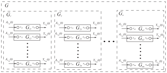
Figure 3: The concatenation decomposition of $G$ as $G=\boxplus_{j=1}^{n}\boxplus_{k=1}^{n}G_{jk}$.

Consider now the model matrix $M$ for the concatenated system $\boxplus_{j=1}^{n}G_{j}$, see Figure 3. With respect to the natural partitioning of $M$ induced by the $G_{jk}$’s (via their concatenation), we label the first $n+1$ rows of $M$ as $s_{00},s_{11},\ldots,s_{1n}$, the next $n$ rows as $s_{21},\ldots,s_{2n}$, the $n$ rows after that $s_{31},s_{32},s_{33},\ldots,s_{3n}$ and so on until the last $n$ rows are labelled $s_{n1},s_{n2},\ldots,s_{nn}$. Similarly, we label the first $n+1$ columns of $M$ as $r_{00},r_{11},\ldots,r_{1n}$, the next $n$ columns as $r_{21},\ldots,r_{2n}$, the $n$ columns after that $r_{31},\ldots,r_{3n}$ and so on until the last $n$ columns $r_{n1},r_{n2}\ldots,r_{nn}$. On occasions, we will need to write a bracket around one of both of the subscripts of $r$ or $s$ (e.g., as in $s_{(n-1)k}$ or $r_{(k+1)(k+1)}$).

Theorem 5

Let the output port $s_{jk}$ be connected to the input port $r_{kj}$ to form an internal edge/channel $e_{jk}=(s_{jk},r_{kj})$ for all $j,k=1,\ldots,n,j\neq k$. Assuming that $\left[\begin{array}[]{cc}-S_{jk}&I\\ I&-S_{kj}\end{array}\right]$ is invertible $\forall j,k=1,\ldots,n,j\neq k$, then the reduced model matrix $M_{\rm red}$ obtained by allowing the delays in all internal edges $\{e_{jk},\;j\neq k\}$ go to zero has parameters given by:

$$S_{\rm red} = {\rm diag}(S_{11},S_{22},\ldots,S_{nn})$$

$$L_{\rm red} = (L_{11}^{T},L_{22}^{T},\ldots,L_{nn}^{T})^{T}$$

$$H_{\rm red} = \sum_{k=1}^{n}H_{k}+\sum_{j=1}^{n-1}\sum_{k=j+1}^{n}\Im\biggl{\{}[\begin{array}[]{cc}L_{jk}^{{\dagger}}&L_{kj}^{{\dagger}}\end{array}]\left[\begin{array}[]{cc}I&-S_{jk}\\ -S_{kj}&I\end{array}\right]^{-1}\left[\begin{array}[]{c}L_{jk}\\ L_{kj}\end{array}\right]\biggr{\}}.$$

The proof of the theorem is given in Appendix A. We will also exploit the following lemma:

Lemma 6

For any real $2\times 2$ matrix $R$ and unitary complex numbers $S_{12}$ and $S_{21}$ satisfying $S_{12}S_{21}\neq 1$, there exist $1\times 2$ complex matrices $K_{1}$ and $K_{2}$ such that $R-\Im\{\frac{S_{12}}{1-S_{12}S_{21}}K_{1}^{{\dagger}}K_{2}+\frac{S_{21}}{1-S_{12}S_{21}}K_{1}^{T}K_{2}^{\#}\}=0$. In fact, a pair $K_{1}$ and $K_{2}$ satisfying this is given by $K_{1}=[\begin{array}[]{cc}\kappa&i\kappa\end{array}]$ with $\kappa$ an arbitrary non-zero real number and $K_{2}=2i[\begin{array}[]{cc}1&0\end{array}][\begin{array}[]{cc}-K_{1}^{{\dagger}}\Delta^{*}&K_{1}^{T}\Delta\end{array}]^{-1}R$, where $\Delta=2\frac{S_{21}-S_{12}^{*}}{|1-S_{12}S_{21}|^{2}}$. Or, alternatively, $K_{2}=[\begin{array}[]{cc}\kappa&i\kappa\end{array}]$ and
$K_{1}=2i[\begin{array}[]{cc}1&0\end{array}][\begin{array}[]{cc}K_{2}^{{\dagger}}\Delta&-K_{2}^{T}\Delta^{*}\end{array}]^{-1}R^{T}$.

See Appendix B for a proof of the lemma. As a consequence of the above theorem and lemma, we have the following result:

Corollary 7

Let $c_{jk}=c_{kj}=1$ whenever $j\neq k$, and $c_{jj}=m$ for all $j,k=1,\ldots,n$. Also, let $S_{jj}=I_{m}$, $S_{kj}=e^{i\theta_{kj}}$ and $S_{jk}=e^{i\theta_{jk}}$ with $\theta_{kj},\theta_{jk}\in[0,2\pi)$ satisfying $\theta_{kj}+\theta_{jk}\neq 0$, $K_{jj}=K_{j}$ and $R_{j}=R_{jj}-2{\rm sym}\biggl{(}\sum_{k=1,k\neq j}^{n}\Im\bigl{\{}\frac{1}{1-S_{jk}S_{kj}}K_{jk}^{{\dagger}}K_{jk}\bigr{\}}\biggr{)}$ ($K_{j}$ and $R_{jj}$ given), where ${\rm sym}(A)=\frac{1}{2}(A+A^{T})$, and the pair $(K_{jk},K_{kj})$ ($j\neq k$) be given by:

$$K_{jk} = [\begin{array}[]{cc}\kappa_{jk}&i\kappa_{jk}\end{array}]$$ (17)

$$K_{kj} = 2i[\begin{array}[]{cc}1&0\end{array}][\begin{array}[]{cc}-K_{jk}^{{\dagger}}\Delta_{jk}^{*}&K_{jk}^{T}\Delta_{jk}\end{array}]^{-1}(R_{jk}-\Im\{K_{j}^{T}K_{k}^{\#}\}),$$ (20)

or

$$K_{kj} = [\begin{array}[]{cc}\kappa_{jk}&i\kappa_{jk}\end{array}]$$ (22)

$$K_{jk} = 2i[\begin{array}[]{cc}1&0\end{array}][\begin{array}[]{cc}K_{kj}^{{\dagger}}\Delta_{jk}&-K_{kj}^{T}\Delta_{jk}^{*}\end{array}]^{-1}(R_{jk}-\Im\{K_{j}^{T}K_{k}^{\#}\})^{T},$$ (25)

where $R_{jk}=R_{kj}^{T}\in\mathbb{R}^{2\times 2}$, $\Delta_{jk}=2\frac{S_{kj}-S_{jk}^{*}}{|1-S_{kj}S_{jk}|^{2}}$ and $\kappa_{jk}$ is an arbitrary non-zero real constant for all $j,k$. Then the reduced Markov model $G_{\rm red}=(S_{\rm red},L_{\rm red},H_{\rm red})$ has the decomposition $G_{\rm red}=\boxplus_{k=0}^{n}G_{\rm red,k}$ with $G_{\rm red,0}=(0,0,H_{\rm red})$ and $G_{\rm red,k}=(S_{kk},L_{kk},0)$ for $k=1,\ldots,n$. Moreover, the network $G_{\rm net}=(S_{\rm net},L_{\rm net},H_{\rm net})$ formed by forming the series product of $G_{\rm red,n}\triangleleft\ldots\triangleleft G_{{\rm red},2}\triangleleft G_{\rm red,1}$ within the concatenated system $G_{\rm red}$ and defined by $G_{\rm net}=G_{\rm red,0}\boxplus(G_{\rm red,n}\triangleleft\ldots\triangleleft G_{{\rm red},2}\triangleleft G_{\rm red,1})$ is a linear quantum stochastic system with parameters given by:

$$S_{\rm net} = I_{m};$$

$$L_{\rm red} = Kx,\;K=[\begin{array}[]{cccc}K_{1}&K_{2}&\ldots&K_{n}\end{array}];$$

$$H_{\rm red} = \frac{1}{2}x^{T}Rx,\;R=[R_{jk}]_{j,k=1,\ldots,n}.$$

In other words, $G_{\rm net}$ realizes a linear quantum stochastic system with the above parameters.

Remark 8

Note that the series connection $G_{\rm red,n}\triangleleft\ldots\triangleleft G_{{\rm red},2}\triangleleft G_{\rm red,1}$ can be viewed as forming and futher eliminating the internal edges $\{(s_{kk},r_{(k+1)(k+1)});\,k=1,\ldots,n-1\}$ in $G_{\rm red}$ or $G$ and, hence, is in essence a special case of a reduced Markov model [15].

The proof of the corollary is given in Appendix C. The corollary shows that an arbitrary linear quantum stochastic system $(I,Kx,\frac{1}{2}x^{T}Rx)$ can be realized by a quantum network $G_{\rm net}$ constructed according to Theorem 5 and the corollary, with an appropriate choice of the parameters $R_{j}$, $K_{jk}$ and $S_{kj}$ ($j\neq k$). From here, any system $(S,Kx,\frac{1}{2}x^{T}Rx)$ can then be easily obtained as $(S,Kx,\frac{1}{2}x^{T}Rx)=(I,Kx,\frac{1}{2}x^{T}Rx)\triangleleft(S,0,0)$. That is, as a cascade of a static network that realizes the unitary scattering matrix $S$ and the system $(I,Kx,\frac{1}{2}x^{T}Rx)$ (see [17, 4]).

Example 9

Consider the realization problem of a two degrees of freedom linear quantum stochastic system $G_{\rm sys}=(I,Kx,1/2x^{T}Rx)$ ($x=(q_{1},p_{1},q_{2},p_{2})^{T}$) with

$$K =[\begin{array}[]{cc}K_{1}&K_{2}\end{array}]=[\begin{array}[]{cccc}3/2&i/2&1&i\end{array}]\;(K_{j}\in\mathbb{C}^{1\times 2},\;j=1,2);$$

$$R =\left[\begin{array}[]{cc}R_{11}&R_{12}\\ R_{12}^{T}&R_{22}\end{array}\right]=\left[\begin{array}[]{cccc}2&0.5&1&1\\ 0.5&3&-1&-1\\ 1&-1&1&0\\ 1&-1&0&1\end{array}\right]\;(R_{jk}\in\mathbb{R}^{2\times 2},\;j,k=1,2).$$

Let $x_{1}=(q_{1},p_{1})^{T}$ and $x_{2}=(q_{2},p_{2})^{T}$. Define $G_{1}=\biggl{(}{\rm diag}(I_{m},S_{12}),\left[\begin{array}[]{c}K_{11}\\ K_{12}\end{array}\right]x_{1},\frac{1}{2}x_{1}^{T}R_{1}x_{1}\biggr{)}$ and $G_{2}=\biggl{(}{\rm diag}(S_{21},I_{m}),\left[\begin{array}[]{c}K_{21}\\ K_{22}\end{array}\right]x_{2},\frac{1}{2}x_{2}^{T}R_{2}x_{2}\biggr{)}$, with certain parameters still to be determined. Choose $\theta_{12}=0$ and $\theta_{21}=\pi/2$, so that $\theta_{12}+\theta_{21}\neq 0$ as required in Corollary 7. Then set $S_{12}=e^{i\theta_{12}}=1$, $S_{21}=e^{i\theta_{21}}=i$, $K_{11}=K_{1}=[\begin{array}[]{cc}3/2&1/2\end{array}]$ and $K_{22}=K_{2}=[\begin{array}[]{cc}1&i\end{array}]$. Compute $\Delta_{12}=2\frac{S_{21}-S_{12}^{*}}{|1-S_{12}S_{21}|^{2}}=-1+i$ and set $\kappa_{12}=1$. Then by Corollary 7 we set $K_{12}=[\begin{array}[]{cc}\kappa_{12}&i\kappa_{12}\end{array}]=[\begin{array}[]{cc}1&i\end{array}]$ and compute $K_{21}=[\begin{array}[]{cc}1.25-0.25i&1.75+0.75i\end{array}]$, $R_{1}=\left[\begin{array}[]{cc}1&0.5\\ 0.5&2\end{array}\right]$ and $R_{2}=-\left[\begin{array}[]{cc}0.625&2\\ 2&2.625\end{array}\right]$. Thus, we have determined all the parameters of $G_{1}$ and $G_{2}$. Labelling the ports of $G_{1}$ and $G_{2}$ according to the convention adopted in this section, $G_{\rm sys}$ can be implemented by concatenating $G_{1}$ and $G_{2}$ and eliminating the internal edges $(s_{12},r_{21})$ and $(s_{21},r_{12})$ to form $G_{\rm red}$ and then eliminating the edge $(s_{11},r_{22})$ (cf. Remark 8) to obtain $G_{\rm net}$ as an approximate realization of $G_{\rm sys}$. This realization is illustrated in Figure 4. $G_{1}$ and $G_{2}$ can then be physical realized in the quantum optics domain following the constructions proposed in [4]. Using the schematic symbols of [4], a quantum optical circuit that is a physical realization of $G_{\rm sys}$ is depicted in Figure 5.

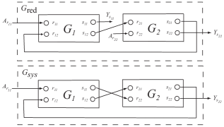
Figure 4: Realization of $G_{\rm sys}$ via a quantum feedback network. In the top figure the internal edges $(s_{12},r_{21})$ and $(s_{21},r_{12})$ are formed and eliminated to obtain a reduced Markov model $G_{\rm red}$. Then in the bottom figure a series (cascade) connection is formed by the eliminating the internal edge $(s_{11},r_{22})$ to realize $G_{\rm sys}$

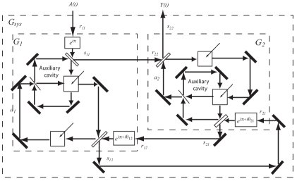
Figure 5: A quantum optical circuit that realizes $G_{\rm sys}$ according to the quantum feedback network in Figure 4; the schematic symbols are taken from [4]. Here $a_{j}=\frac{q_{j}+ip_{j}}{2}$ is cavity mode of the optical cavity around which the physical realization of the oscillator $G_{j}$ is based, $j=1,2$. The dashed box labelled $G_{j}$ is the part of the circuit realizing $G_{j}$, and the input and output ports of $G_{j}$ are indicated by their respective labels. The value of the parameters of devices in this circuit can be determined according to [4].

7 Synthesis of passive systems

Let us now consider a special class of linear quantum stochastic systems that we shall refer to as passive linear quantum stochastic systems, for a reason that is explained below, and show that any such system can be built from passive components. This class of systems has also been considered in, e.g., [18, 19].

For $k=1,\ldots,n$ let $a_{k}=\frac{q_{k}+ip_{k}}{2}$ be the annihilation operators for mode $k$ and define $a=(a_{1},\ldots,a_{n})^{T}$. Then $a$ satisfies the CCR

$$\left[\begin{array}[]{c}a\\ a^{\#}\end{array}\right]\left[\begin{array}[]{cc}a^{{\dagger}}&a^{T}\end{array}\right]-\left(\left[\begin{array}[]{c}a^{\#}\\ a\end{array}\right]\left[\begin{array}[]{cc}a^{T}&a^{{\dagger}}\end{array}\right]\right)^{T}$$

$$\quad={\rm diag}(I_{n},-I_{n}).$$

Moreover, note that:

$$\left[\begin{array}[]{c}a\\ a^{\#}\end{array}\right]=\left[\begin{array}[]{c}\Sigma\\ \Sigma^{\#}\end{array}\right]x;\quad$$

where

$$\Sigma=\left[\begin{array}[]{ccccccc}\frac{1}{2}&i\frac{1}{2}&0&0&0&\ldots&0\\ 0&0&\frac{1}{2}&i\frac{1}{2}&0&\ldots&0\\ \vdots&\ddots&\ddots&\ddots&\ddots&\ddots&\vdots\\ 0&\ldots&\ldots&\ldots&0&\frac{1}{2}&i\frac{1}{2}\end{array}\right].$$

We also make note that $\left[\begin{array}[]{c}\Sigma\\ \Sigma^{\#}\end{array}\right]^{-1}=2\left[\begin{array}[]{cc}\Sigma^{{\dagger}}&\Sigma^{T}\end{array}\right]$ and therefore we have

$$x=\left[\begin{array}[]{c}\Sigma\\ \Sigma^{\#}\end{array}\right]^{-1}\left[\begin{array}[]{c}a\\ a^{\#}\end{array}\right]=2\left[\begin{array}[]{cc}\Sigma^{{\dagger}}&\Sigma^{T}\end{array}\right]\left[\begin{array}[]{c}a\\ a^{\#}\end{array}\right].$$

An $n$ degrees of freedom system $G=(S,Kx,\frac{1}{2}x^{T}Rx)$ is said to be passive if we may write $H=\frac{1}{2}x^{T}Rx=\frac{1}{2}a^{{\dagger}}\tilde{R}a+c$ and $L=Kx=\tilde{K}a$ for some real constant $c$ (arising due the commutation relations among the canonical operators), some complex $n\times n$ Hermitian matrix $\tilde{R}$ and some complex $m\times n$ ($m$ here again denotes the number of input and output fields in and out of $G$) matrix $\tilde{K}$. Here the term passive for such systems is physically motivated. By the given definition, the Hamiltonian $H$ contains no terms of the form $c_{1}a_{j}^{2}$, $c_{2}a_{k}^{*2}$, $c_{3}a_{j}a_{k}$ and $c_{4}a_{j}^{*}a_{k}^{*}$ and the coupling operator $L$ contains no terms of the form $c_{5}a_{k}^{*}$ (here $c_{1},\ldots,c_{5}$ denote arbitrary complex constants), with the indexes $j$ and $k$ running over $1,\ldots,n$. These terms are precisely the terms that require an external source of quanta (i.e., an external pump beam) to realize (see, e.g., [4]) and cannot be implemented only by passive components like mirrors, beamsplitters and phase shifters. The absence of such “active” terms is the reason we refer to this class of systems as passive.

Let us write $\frac{1}{2}a^{{\dagger}}\tilde{R}a$ and $\tilde{K}a$ in the following way:

$$\frac{1}{2}a^{{\dagger}}\tilde{R}a = \frac{1}{2}\left[\begin{array}[]{cc}a^{{\dagger}}&a^{T}\end{array}\right]\left[\begin{array}[]{cc}\frac{1}{2}\tilde{R}&0_{n\times n}\\ 0_{n\times n}&\frac{1}{2}\tilde{R}^{\#}\end{array}\right]\left[\begin{array}[]{c}a\\ a^{\#}\end{array}\right]-\frac{1}{4}\sum_{j=1}^{n}\tilde{R}_{jj}$$

$$= \frac{1}{2}x^{T}\Re\{\Sigma^{{\dagger}}\tilde{R}\Sigma\}x-\frac{1}{4}\sum_{j=1}^{n}\tilde{R}_{jj}$$

$$\tilde{K}a = \tilde{K}\left[\begin{array}[]{cc}I&0\end{array}\right]\left[\begin{array}[]{c}a\\ a^{\#}\end{array}\right]=\tilde{K}\Sigma x.$$

Therefore, $H=\frac{1}{2}x^{T}Rx$ with $R=\Re\{\Sigma^{{\dagger}}\tilde{R}\Sigma\}$, and $L=Kx$ with $K=\tilde{K}\Sigma$. It is easy to see from this that for any passive system the block diagonal elements $R_{jj}$ must be diagonal matrices of the form $\lambda_{j}I_{2}$ with $\lambda_{j}\in\mathbb{R}$, the off diagonal block elements $R_{jk}$ are real $2\times 2$ matrices of the form $R_{jk}=\left[\begin{array}[]{cc}\alpha_{jk}&\beta_{jk}\\ -\beta_{jk}&\alpha_{jk}\end{array}\right]$ for some real numbers $\alpha_{jk}$ and $\beta_{jk}$, and the coupling matrix $K_{j}$ to $x_{j}$ is of the form $K_{j}=[\begin{array}[]{cc}\gamma_{j}&i\gamma_{j}\end{array}]$ for some complex number $\gamma_{j}$. One would hope that a passive system can be synthesized using purely passive components and the next theorem states that this is indeed the case.

Theorem 10

Let $G_{\rm sys}=(S,L,H)$ be passive. Then the systems $\{G_{j};j=1,\ldots,n\}$ constructed according to Corollary 7 are all also passive.

The proof of the theorem can be found in Appendix D. We now conclude this section with an example of a passive system synthesis.

Example 11

Consider the realization problem of a passive two degrees of freedom linear quantum stochastic system $G_{\rm sys}=(I,Kx,1/2x^{T}Rx)$ ($x=(q_{1},p_{1},q_{2},p_{2})^{T}$) with

$$K =[\begin{array}[]{cc}K_{1}&K_{2}\end{array}]=[\begin{array}[]{cccc}-3+i&-1-3i&1&i\end{array}]\;(K_{j}\in\mathbb{C}^{1\times 2},\;j=1,2);$$

$$R =\left[\begin{array}[]{cc}R_{11}&R_{12}\\ R_{12}^{T}&R_{22}\end{array}\right]=\left[\begin{array}[]{cccc}2&0&1&4\\ 0&2&-4&1\\ 1&-4&1&0\\ 4&1&0&1\end{array}\right]\;(R_{jk}\in\mathbb{R}^{2\times 2},\;j,k=1,2).$$

Setting $\kappa_{12}=1$, $S_{12}=1$, $S_{21}=i$ and $K_{12}=[\begin{array}[]{cc}\kappa_{12}&i\kappa_{12}\end{array}]=[\begin{array}[]{cc}1&i\end{array}]$, we obtain from Corollary 7, $K_{11}=K_{1}$, $K_{22}=K_{2}$, $K_{21}=[\begin{array}[]{cc}0.5-0.5i&0.5+0.5i\end{array}]$, $R_{1}=0_{2\times 2}$ and $R_{2}=0.5I_{2}$. An entirely passive optical circuit that realizes $G_{\rm sys}$ is shown in Figure 6.

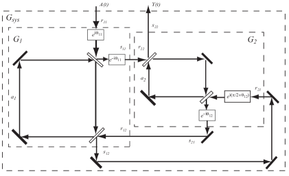
Figure 6: A quantum optical circuit that realizes the passive system $G_{\rm sys}$ of this example. The circuit consists of only passive optical components: mirrors and phase shifters. Here $\theta_{11}=\pi-\arctan(1/3)$ and $\theta_{21}=-\frac{\pi}{4}$, and the values of all other parameters of devices in this circuit can be determined according to [4].

8 Conclusions

In this paper we have developed a new method or algorithm for systematically synthesizing an arbitrary linear quantum stochastic system via a suitable quantum feedback network. In the synthesis, all interactions between the oscillators constituting the network are facilitated only by quantum fields. In particular, it offers an alternative to the challenging task of implementing direct bilinear interaction Hamiltonians that was required in the approach of [4]. Moreover, it is shown that if the system is passive then with the new algorithm it can be realized using only passive components. It is clearly also possible to combine the present algorithm with that of [4] to form a hybrid synthesis method.

Current interest in quantum information science, and quantum control in particular, provides much impetus for extending network synthesis theory to the quantum domain as a significant direction in which to further develop circuit and systems theory. The quantum synthesis results presented here could be of particular relevance for the design and systematic physical realization of photonics based monolithic linear open quantum circuits which may form an important sub-system of future continuous variable quantum information processing systems.

Appendix A Proof of Theorem 5

For this proof, it will be convenient to interchange some rows and columns of the model matrix $M$ to form another model matrix $\tilde{M}$ to avoid complicated book keeping and thus reduce unnecessary clutter. Here by “rows” and “columns” we mean, respectively, block rows and block columns of $M$ formed with respect to its specifed partitioning. This interchange is as follows.

First, we permute rows of $M$ such that the first $2n-1$ rows from top to bottom are the rows labelled (while column labels are kept fixed as they are) $s_{00},s_{12},s_{21},s_{13},s_{31},\ldots,s_{1n},s_{n1}$, the next $2(n-2)$ rows respectively are the rows labelled $s_{23},s_{32},s_{24},s_{42},\ldots,s_{2n},s_{n2}$, the $2(n-3)$ rows after that are respectively the rows labelled $s_{34},s_{43},s_{35},s_{53},\ldots,s_{3n},s_{n3}$ and so on in the same pattern until we get to the last $n$ rows that are respectively those rows labelled $s_{11},s_{22},\ldots,s_{nn}$. Call the intermediate matrix resulting from this row permutation $\hat{M}$. Then fixing the row labels of $\hat{M}$, we permute its columns such that the first $2n-1$ columns from left to right are respectively the columns of $\hat{M}$ labelled $r_{00},r_{12},r_{21},r_{13},r_{31},\ldots,r_{1n},r_{n1}$, the next $2(n-2)$ columns are respectively the columns labelled $r_{23},r_{32},r_{24},r_{42},\ldots,r_{2n},r_{n2}$, the $2(n-3)$ rows after are respective the columns labelled $r_{34},r_{43},r_{35},r_{53},\ldots,r_{3n},r_{n3}$, and so on in the same pattern until the final $n$ columns that are respectively the columns labelled $r_{11},r_{22},\ldots,r_{nn}$. The resulting matrix after this permutation of columns is $\tilde{M}$.

It is important to note here that since the same permutation is applied to the rows and columns, $M$ and $\tilde{M}$ are model matrix representations of the same physical system, save for a mere rearrangement of the ordering or indexing of the fields and ports. That is to say that if $M$ is the model matrix of $G=(S,L,H)$ then $\tilde{M}$ is the model matrix of $\tilde{G}=(PSP^{T},PL,H)$ for some suitable constant real permutation matrix $P$, while it is clear that $G$ and $\tilde{G}$ are representations of the same physical system. Thus with the same internal connections made, a reduced model matrix for $\tilde{M}$ is also a reduced model matrix for $M$, up to a possible relabelling of uneliminated ports.

Let $\tilde{L}=PL$ and $\tilde{S}=PSP^{T}$. Then $\tilde{L}$ can be partitioned as $\tilde{L}=(\tilde{L}_{\rm i}^{T},\tilde{L}_{\rm e}^{T})^{T}$, where $\tilde{L}_{\rm i}$ is the first $n(n-1)+1$ rows of $\tilde{L}$, while $\tilde{L}_{\rm e}$ is the last $n$ rows of $\tilde{L}$. They are of the form:

$$\tilde{L}_{\rm i} = (L_{12}^{T},L_{21}^{T},L_{13}^{T},L_{31}^{T},\ldots,L_{1n}^{T},L_{n1}^{T},L_{23}^{T},L_{32}^{T},L_{24}^{T},L_{42}^{T},\ldots,L_{2n}^{T},L_{n2}^{T},\ldots,$$

$$L_{(n-2)(n-1)}^{T},L_{(n-1)(n-2)}^{T},L_{(n-2)n}^{T},L_{n(n-2)}^{T},L_{(n-1)n}^{T},L_{n(n-1)}^{T})^{T}$$

$$\tilde{L}_{\rm e} = (L_{11}^{T},L_{22}^{T},\ldots,L_{nn}^{T})^{T}.$$

Similarly, $\tilde{S}$ can be partitioned as $\tilde{S}=\left[\begin{array}[]{cc}\tilde{S}_{\rm ii}&\tilde{S}_{\rm ie}\\ \tilde{S}_{\rm ei}&\tilde{S}_{\rm ee}\end{array}\right]$, with $\tilde{S}_{\rm ii}$ and $\tilde{S}_{\rm ee}$ being block diagonal:

$$\tilde{S}_{\rm ii} = {\rm diag}(S_{12},S_{21},S_{13},S_{31},\ldots,S_{1n},S_{n1},S_{23},S_{32},S_{24},S_{42},\ldots,S_{2n},S_{n2},\ldots,$$

$$S_{(n-2)(n-1)},S_{(n-1)(n-2)},S_{(n-2)n},S_{n(n-2)},S_{(n-1)n},S_{n(n-1)})$$

$$\tilde{S}_{\rm ee} = {\rm diag}(S_{11},S_{22},\ldots,S_{nn}),$$

and $\tilde{S}_{\rm ei}$ and $\tilde{S}_{\rm ie}$ both being zero matrices. Then $\tilde{M}$ has the partitioning of the form (14) by identifying $S_{\rm ii}$, $S_{\rm ie}$, $S_{\rm ei}$, $S_{\rm ee}$, $L_{\rm i}$ and $L_{\rm e}$ with $\tilde{S}_{\rm ii}$, $\tilde{S}_{\rm ie}$, $\tilde{S}_{\rm ei}$, $\tilde{S}_{\rm ee}$ and $\tilde{L}_{\rm i}$ and $\tilde{L}_{\rm e}$, respectively. The reduced model matrix resulting from the subsequent simultaneous elimination of all internal edges $(s_{jk},r_{kj})$ $j,k=1,\ldots,n,j\neq k$, can be conveniently determined by using the adjacency matrix $\eta$ defined by:

$$\eta = {\rm diag}\left(\left[\begin{array}[]{cc}0&I_{c_{12}}\\ I_{c_{21}}&0\end{array}\right],\left[\begin{array}[]{cc}0&I_{c_{13}}\\ I_{c_{31}}&0\end{array}\right],\ldots,\right.$$

$$\quad\left.\left[\begin{array}[]{cc}0&I_{c_{1n}}\\ I_{c_{n1}}&0\end{array}\right],\left[\begin{array}[]{cc}0&I_{c_{23}}\\ I_{c_{32}}&0\end{array}\right],\left[\begin{array}[]{cc}0&I_{c_{24}}\\ I_{c_{42}}&0\end{array}\right],\right.$$

$$\quad\left.\ldots,\left[\begin{array}[]{cc}0&I_{c_{2n}}\\ I_{c_{n2}}&0\end{array}\right],\ldots,\left[\begin{array}[]{cc}0&I_{c_{(n-1)n}}\\ I_{c_{(n-1)n}}&0\end{array}\right]\right).$$

(Recall that $c_{jk}=c_{kj}$). Hence, according to Theorem 3, the reduced model matrix $\tilde{M}_{\rm red}$ obtained after elimination of the internal edges $\{(s_{jk},r_{kj});\,j,k=1,\ldots,n,j\neq k\}$, has parameters given by (recalling that $\tilde{S}_{\rm ei}$ and $\tilde{S}_{\rm ie}$ are zero matrices):

$$\tilde{S}_{\rm red} = \tilde{S}_{\rm ee}+\tilde{S}_{\rm ei}(\eta-\tilde{S}_{\rm ii})^{-1}\tilde{S}_{\rm ie}=\tilde{S}_{\rm ee},$$

$$\tilde{L}_{\rm red} = \tilde{L}_{\rm e}+\tilde{S}_{\rm ei}(\eta-\tilde{S}_{\rm ii})^{-1}\tilde{L}_{\rm i}=\tilde{L}_{\rm e}$$

$$\tilde{H}_{\rm red} = \sum_{k=1}^{n}H_{k}+\sum_{j={\rm i,e}}\Im\{\tilde{L}_{j}^{{\dagger}}\tilde{S}_{j{\rm i}}(\eta-\tilde{S}_{\rm ii})^{-1}\tilde{L}_{\rm i}\}$$

$$= \sum_{k=1}^{n}H_{k}+\Im\{\tilde{L}_{\rm i}^{{\dagger}}\tilde{S}_{{\rm ii}}(\eta-\tilde{S}_{\rm ii})^{-1}\tilde{L}_{\rm i}\}$$

$$= \sum_{k=1}^{n}H_{k}+\Im\{\tilde{L}_{\rm i}^{{\dagger}}\eta(\eta-\tilde{S}_{\rm ii})^{-1}\tilde{L}_{\rm i}\}$$

$$= \sum_{k=1}^{n}H_{k}+\sum_{j=1}^{n-1}\sum_{k=j+1}^{n}\Im\biggl{\{}[\begin{array}[]{cc}L_{jk}^{{\dagger}}&L_{kj}^{{\dagger}}\end{array}]\left[\begin{array}[]{cc}I&-S_{jk}\\ -S_{kj}&I\end{array}\right]^{-1}\left[\begin{array}[]{c}L_{jk}\\ L_{kj}\end{array}\right]\biggr{\}}$$

Since $M$ and $\tilde{M}$ are model matrix representations of the same physical system and the external fields have the same ordering and labelling in both representations, the reduced model matrix of $M_{\rm red}$ and $\tilde{M}_{\rm red}$ of $M$ and $\tilde{M}$, respectively, after elimination of internal edges $(s_{jk},r_{kj})$, coincide. Hence, also the linear quantum stochastic systems $G_{\rm red}$ and $\tilde{G}_{\rm red}$ associated with $M$ and $\tilde{M}$, respectively, coincide. This completes the proof. $\Box$

Appendix B Proof of Lemma 6

We begin by noting that

$$\Im\{\frac{S_{12}}{1-S_{12}S_{21}}K_{1}^{{\dagger}}K_{2}+\frac{S_{21}}{1-S_{12}S_{21}}K_{1}^{T}K_{2}^{\#}\}=\frac{1}{2i}[\begin{array}[]{cc}-K_{1}^{{\dagger}}\Delta^{*}&K_{1}^{T}\Delta\end{array}]\left[\begin{array}[]{c}K_{2}\\ K_{2}^{\#}\end{array}\right],$$

with $\Delta=\frac{S_{21}}{1-S_{21}S_{12}}-\frac{S_{12}^{*}}{1-S_{21}^{*}S_{12}^{*}}=2\frac{S_{21}-S_{12}^{*}}{|1-S_{21}S_{12}|^{2}}$ (exploiting the fact that $S_{12}S_{12}^{*}=1=S_{21}S_{21}^{*}$). Now set $K_{1}=[\begin{array}[]{cc}\kappa&i\kappa\end{array}]$ for an arbitrary non-zero real constant $\kappa$, and note that $S_{21}S_{12}\neq 1$ implies that $\Delta\neq 0$ and:

$$[\begin{array}[]{cc}-K_{1}^{{\dagger}}\Delta^{*}&K_{1}^{T}\Delta\end{array}]^{-1} = \left[\begin{array}[]{cc}-\kappa\Delta^{*}&\kappa\Delta\\ i\kappa\Delta^{*}&i\kappa\Delta\end{array}\right]^{-1}=-\frac{1}{2i\kappa^{2}|\Delta|^{2}}\left[\begin{array}[]{cc}i\kappa\Delta&-\kappa\Delta\\ -i\kappa\Delta^{*}&-\kappa\Delta^{*}\end{array}\right],$$

and therefore for any real matrix $V$, $2i[\begin{array}[]{cc}-K_{1}^{{\dagger}}\Delta^{*}&K_{1}^{T}\Delta\end{array}]^{-1}V=\left[\begin{array}[]{c}Z\\ Z^{\#}\end{array}\right]$ for some complex row vector $Z$. Therefore, given any $R$ we see that we may solve the equation

$$[\begin{array}[]{cc}-K_{1}^{{\dagger}}\Delta^{*}&K_{1}^{T}\Delta\end{array}]\left[\begin{array}[]{c}K_{2}\\ K_{2}^{\#}\end{array}\right]=2iR,$$

for $K_{2}$ and this solution is as given in the statement of the corollary.

Alternatively, we could also have started by setting $K_{2}=[\begin{array}[]{cc}\kappa&i\kappa\end{array}]$ and analogously solving for $K_{1}$ for a given $R$. It is then an easy exercise that the solution for $K_{1}$ in this case is as stated in the corollary. $\Box$

Appendix C Proof of Corollary 7

With $c_{jk}$, $S_{jk}$, $R_{jk}$ and $K_{jk}$, $j,k=1,\ldots,n$, as defined in the statement of the corollary, from Theorem 5 and Lemma 6 we have that $S_{\rm red}=I_{nm}$, $L_{\rm red}=(L_{11}^{T},L_{22}^{T},\ldots,L_{nn}^{T})^{T}$ with $L_{jj}=K_{j}x_{j}$, and

$$H_{\rm red} = \sum_{j=1}^{n}H_{j}+\sum_{j=1}^{n-1}\sum_{k=j+1}^{n}\Im\{[\begin{array}[]{cc}L_{jk}^{{\dagger}}&L_{kj}^{{\dagger}}\end{array}]\left[\begin{array}[]{cc}1&-S_{jk}\\ -S_{kj}&1\end{array}\right]^{-1}\left[\begin{array}[]{c}L_{jk}\\ L_{kj}\end{array}\right]\}.$$

Expanding, we have:

$$H_{\rm red} = \frac{1}{2}\sum_{j=1}^{n}x_{j}^{T}R_{j}x_{j}+\sum_{j=1}^{n-1}\sum_{k=j+1}^{n}\Im\biggl{\{}\frac{1}{1-S_{jk}S_{kj}}\cdot$$

$$\;(L_{jk}^{{\dagger}}L_{jk}+S_{jk}L_{jk}^{{\dagger}}L_{kj}+S_{kj}L_{kj}^{{\dagger}}L_{jk}+L_{kj}^{{\dagger}}L_{kj})\biggr{\}}$$

$$= \frac{1}{2}\sum_{j=1}^{n}x_{j}^{T}\biggl{(}R_{j}+2{\rm sym}\biggl{(}\sum_{k=1,k\neq j}^{n}\Im\{\frac{K_{jk}^{{\dagger}}K_{jk}}{1-S_{jk}S_{kj}}\}\biggr{)}\biggr{)}x_{j}$$

$$\;+\sum_{j=1}^{n-1}\sum_{k=j+1}^{n}x_{j}^{T}\Im\{\frac{S_{jk}}{1-S_{jk}S_{kj}}K_{jk}^{{\dagger}}K_{kj}+\frac{S_{kj}}{1-S_{jk}S_{kj}}K_{jk}^{T}K_{kj}^{\#}\}x_{k}$$

$$= \frac{1}{2}\sum_{j=1}^{n}x_{j}^{T}R_{jj}x_{j}+\sum_{j=1}^{n-1}\sum_{k=j+1}^{n}x_{j}^{T}\bigl{(}R_{jk}-\Im\{K_{j}^{T}K_{k}^{\#}\}\bigr{)}x_{k}$$

$$= \frac{1}{2}x^{T}Rx-\sum_{j=1}^{n-1}\sum_{k=j+1}^{n}x_{j}^{T}\Im\{K_{j}^{T}K_{k}^{\#}\}x_{k},$$

where ${\rm sym}(A)=\frac{1}{2}(A+A^{T})$, and $R=[R_{jk}]_{j,k=1,\ldots,n}$ and $R_{kj}=R_{jk}^{T}$. From this it is clear that using the concatenation product we can decompose $G_{\rm red}$ as $G_{\rm red}=(0,0,H_{\rm red})\boxplus\boxplus_{j=1}^{n}(I_{m},L_{jj},0)$. Let $G_{{\rm red},0}=(0,0,H_{\rm red})$ and $G_{{\rm red},j}=(I_{m},L_{jj},0)$, $j=1,\ldots,n$. Now, using the series product rule (cf. Section 2), we easily compute that

$$G_{\rm net} = G_{{\rm red},0}\boxplus(G_{{\rm red},n}\triangleleft\ldots\triangleleft G_{{\rm red},2}\triangleleft G_{{\rm red},1})$$

$$= \biggl{(}0,0,\frac{1}{2}x^{T}Rx-\sum_{j=1}^{n-1}\sum_{k=j+1}^{n}x_{j}^{T}\Im\{K_{j}^{T}K_{k}^{\#}\}x_{k}\biggr{)}\boxplus$$

$$\biggl{(}I_{m},[\begin{array}[]{cccc}K_{1}&K_{2}&\ldots&K_{n}\end{array}]x,\sum_{j=1}^{n-1}\sum_{k=j+1}^{n}x_{j}^{T}\Im\{K_{j}^{T}K_{k}^{\#}\}x_{k}\biggr{)}$$

$$= \biggl{(}I_{m},[\begin{array}[]{cccc}K_{1}&K_{2}&\ldots&K_{n}\end{array}]x,\frac{1}{2}x^{T}Rx\biggr{)}.$$

Therefore, $G_{\rm net}$ realizes a linear quantum stochastic system with parameters $S_{\rm net}$, $L_{\rm net}$ and $H_{\rm net}$, as claimed. $\Box$

Appendix D Proof of Theorem 10

By the passivity of $G_{\rm sys}$, we immediately see that $K_{jj}=K_{j}$ is already of the form required for passivity of $G_{j}$, and the matrix $R_{jk}-\Im\{K_{j}^{T}K_{k}^{\#}\}$ is a $2\times 2$ real matrix of the form $\left[\begin{array}[]{cc}\alpha^{\prime}_{jk}&\beta^{\prime}_{jk}\\ -\beta^{\prime}_{jk}&\alpha^{\prime}_{jk}\end{array}\right]$ for some $\alpha^{\prime}_{jk},\beta^{\prime}_{jk}\in\mathbb{R}$, whenever $j\neq k$. Let $\kappa_{jk}$, $S_{jk}$ and $S_{kj}$ be chosen according to Corollary 7. Set $K_{jk}$ according to the first equality of (20). Then some straightforward algebra shows that $K_{kj}$ given by the second equality of (20) is of the form $K_{kj}=[\begin{array}[]{cc}\gamma^{\prime}_{kj}&i\gamma^{\prime}_{kj}\end{array}]$ for some $\gamma^{\prime}_{kj}\in\mathbb{C}$, just like $K_{jk}$. The same holds true if one chooses the alternative of setting $K_{kj}$ according to the first equality of (25) and computing $K_{jk}$ according to the second equality of (25). Finally, given this special form of $K_{jk}$, it is easily inspected that ${\rm sym}\bigl{(}\Im\{\frac{1}{1-S_{jk}S_{kj}}K_{jk}^{{\dagger}}K_{jk}\}\bigr{)}$ is a diagonal matrix of the form $\lambda_{jk}I_{2}$ for some $\lambda_{jk}\in\mathbb{R}$ for all $j,k,j\neq k$ (recall that ${\rm sym}(A)=\frac{1}{2}(A+A^{T})$), and since $R_{jj}$ is also diagonal of this form (again from the passivity of $G_{\rm sys}$) we have that $R_{j}=R_{jj}-2\sum_{k=1,k\neq j}^{n}{\rm sym}\bigl{(}\Im\{\frac{1}{1-S_{jk}S_{kj}}K_{jk}^{{\dagger}}K_{jk}\}\bigr{)}$ is again of the same form, for all $j$. Therefore, it now follows that each sub-system $G_{j}$ of Section 6 with parameters determined according to Corollary 7 is passive. This completes the proof.

References

- [1] S. C. Edwards and V. P. Belavkin, “Optimal quantum filtering and quantum feedback control,” August 2005. [Online]. Available: http://arxiv.org/pdf/quant-ph/0506018
- [2] M. R. James, H. I. Nurdin, and I. R. Petersen, “ control of linear quantum stochastic systems,” IEEE Trans. Automat. Contr., vol. 53, no. 8, pp. 1787–1803, 2008.
- [3] H. I. Nurdin, M. R. James, and I. R. Petersen, “Coherent quantum LQG control,” 2009, accepted for publication, Automatica. [Online]. Available: http://arxiv.org/pdf/0711.2551v1 (preprint)
- [4] H. I. Nurdin, M. R. James, and A. C. Doherty, “Network synthesis of linear dynamical quantum stochastic systems,” June 2008, provisionally acceptable for publication subject to some minor revisions, SIAM Journal on Control and Optimization (2009). [Online]. Available: http://arxiv.org/abs/0806.4448v1 (preprint)
- [5] C. Gardiner and P. Zoller, Quantum Noise: A Handbook of Markovian and Non-Markovian Quantum Stochastic Methods with Applications to Quantum Optics, 2nd ed., ser. Springer Series in Synergetics. Springer, 2000.
- [6] B. Yurke and J. S. Denker, “Quantum network theory,” Phys. Rev. A, vol. 29, no. 3, pp. 1419–1437, 1984.
- [7] S. Mancini, “Markovian feedback to control continuous-variable entanglement,” Phys. Rev. A, vol. 73, no. 010304(R), pp. 010 304–1–010 304–4, 2006.
- [8] S. Mancini and H. Wiseman, “Optimal control of entanglement via quantum feedback,” Phys. Rev.A, vol. 75, no. 012330, pp. 012 330–1–012 330–9, 2007.
- [9] N. Yamamoto, H. I. Nurdin, M. R. James, and I. R. Petersen, “Avoiding entanglement sudden death via measurement feedback control in a quantum network,” Phys. Rev. A, vol. 78, p. 042339, 2008.
- [10] S. Lloyd and S. L. Braunstein, “Quantum computation over continuous variables,” Phys. Rev. Lett, vol. 82, no. 8, pp. 1785–1787, February 1999.
- [11] M. Yanagisawa and H. Kimura, “Transfer function approach to quantum control-part II: Control concepts and applications,” IEEE Trans. Automatic Control, vol. 48, no. 12, pp. 2121–2132, 2003.
- [12] H. Mabuchi, “Coherent-feedback quantum control with a dynamic compensator,” Phys. Rev. A, vol. 78, p. 032323, 2008.
- [13] J. P. Dowling and G. J. Milburn, “Quantum technology: The second quantum revolution,” Philosophical Transactions: Mathematical, Physical and Engineering Sciences, vol. 361, no. 1809, pp. 1655–1674, August 2003.
- [14] B. D. O. Anderson and S. Vongpanitlerd, Network Analysis and Synthesis: A Modern Systems Theory Approach, ser. Networks Series. Prentice-Hall, Inc., 1973.
- [15] J. Gough and M. R. James, “Quantum feedback networks: Hamiltonian formulation,” 2008, to appear in Communications in Mathematical Physics. [Online]. Available: http://arxiv.org/pdf/0804.3442v3 (preprint)
- [16] H. I. Nurdin, “Topics in classical and quantum linear stochastic systems,” Ph.D. dissertation, The Australian National University, April 2007.
- [17] J. Gough and M. R. James, “The series product and its application to quantum feedforward and feedback networks,” 2009, IEEE Transactions on Automatic Control, to appear. [Online]. Available: http://arxiv.org/abs/0707.0048v3
- [18] J. Gough, R. Gohm, and M. Yanagisawa, “Linear quantum feedback networks,” Phys. Rev. A, vol. 78, p. 061204, 2008.
- [19] A. I. Maalouf and I. R. Petersen, “Coherent control for a class of linear complex quantum systems,” 2009, to be published in Proceedings of the 2009 American Control Conference (St. Louis, MO, June 2009).