Elastic-Net Regularization: Error estimates and Active Set Methods

Abstract

This paper investigates theoretical properties and efficient numerical algorithms for the so-called elastic-net regularization originating from statistics, which enforces simultaneously $\ell^{1}$ and $\ell^{2}$ regularization. The stability of the minimizer and its consistency are studied, and convergence rates for both a priori and a posteriori parameter choice rules are established. Two iterative numerical algorithms of active set type are proposed, and their convergence properties are discussed. Numerical results are presented to illustrate the features of the functional and algorithms.

1 Introduction

In recent years, minimization problems involving so-called sparsity constraints have gained considerable interest. Sparsity has been found as a powerful tool and recognized as an important structure in many disciplines, e.g. geophysical problems [26, 22], imaging science [12], statistics [27] and signal processing [7, 6]. The setting is often as following: Let $\mathcal{H}_{1}$ and $\mathcal{H}_{2}$ be two Hilbert spaces and let $\mathcal{H}_{1}$ be equipped with an orthonormal basis $\{\varphi_{i}\in\mathcal{H}_{1}:i\in\mathbb{N}\}$ (or an overcomplete dictionary). Then, for given linear and continuous operator $K:\mathcal{H}_{1}\rightarrow\mathcal{H}_{2}$, data $y^{\delta}\in\mathcal{H}_{2}$ and regularization parameter $\alpha>0$, we seek the minimizer of the functional

$$\Psi(x)=\frac{1}{2}\|Kx-y^{\delta}\|^{2}+\alpha\sum_{i}|\langle x,\varphi_{i}\rangle|.$$

Here $y^{\delta}$ is an observational version of the exact data $y^{\dagger}$ and satisfies an estimate of the form $\|y^{\delta}-y^{\dagger}\|\leq\delta$. With the help of the basis expansion, the problem can be reformulated as

$$\min_{x\in\ell^{2}}\Psi(x)\quad\text{with}\quad\Psi(x)=\frac{1}{2}\|Kx-y^{\delta}\|^{2}+\alpha\|x\|_{\ell^{1}},$$ (1)

by abusing the notation $x$ for the sequence of expansion coefficients $\{x_{i}:=\langle x,\varphi_{i}\rangle\}$ and $K$ for the operator $\{x_{i}\}\mapsto K\sum_{i}x_{i}\varphi_{i}$ mapping from $\ell^{2}$ to $\mathcal{H}_{2}$.

Because of its central importance in inverse problems and signal processing, the efficient minimization of the functional $\Psi$ has received much attention, and a wide variety of numerical algorithms, e.g. iterated thresholding/shrinkage [9, 3], gradient projection [13, 29], fixed point continuation [16], semismooth Newton method (SSN) [15] and feature sign search (FSS) [21], have been proposed. Both SSN and FSS are of active set type, and have delivered favorable performance compared to the above-mentioned first-order methods. However, they often require inverting potentially ill-conditioned operators, and thus lead to numerical problems. One possible remedy is to regularize the inversion, e.g. by Tikhonov regularization. On the other hand, recent studies [23, 14] show the regularizing property of the functional $\Psi$ and under suitable source conditions also the convergence rate of its minimizer $x_{\alpha}^{\delta}$ to the true solution $x^{\dagger}$ of the form

$$\|x_{\alpha}^{\delta}-x^{\dagger}\|_{\ell^{2}}=\mathcal{O}(\delta).$$

However, the involved constant may be astronomically large. In other words, the ill-posed problem has been turned into a well-posed but ill-conditioned one, and this is in accordance with inverting ill-conditioned operators. In this paper we propose to address both issues by Tikhonov regularization, i.e. considering a functional of the form

$$\Phi_{\alpha,\beta}(x)=\frac{1}{2}\|Kx-y^{\delta}\|^{2}+\alpha\|x\|_{\ell^{1}}+\frac{\beta}{2}\|x\|_{\ell^{2}}^{2}.$$

We will show that this functional leads to more stable active-set algorithms and provides improved error estimates. We note that it also arises by Moreau-Yosida regularization of the Fenchel dual of the functional $\Psi$.

The functional $\Phi_{\alpha,\beta}$ is also used in statistics under the name elastic-net regularization [30]. It is motivated by the following observation: The functional $\Psi$ delivers undesirable results for problems where there are highly correlated features and we need to identify all relevant ones, e.g. microarray data analysis, in that it tends to select only one feature out of the relevant group instead of all relevant features of the group [30], i.e. it fails to identify the group structure. Zou and Hastie [30] proposed introducing an extra $\ell^{2}$ regularization term, i.e. the functional $\Phi_{\alpha,\beta}$, in the hope of retrieving correctly the whole relevant group, and numerically confirmed the desired property of the functional for both simulation studies and real-data applications. For further statistical motivations we refer to reference [30]. Quite recently, De Mol et al. [10] showed some interesting theoretical properties of the functional $\Phi_{\alpha,\beta}$, but their focus is fundamentally different from ours: Their main concern is on its statistical properties in the framework of learning theory and an algorithm of iterated shrinkage type, whereas ours is within the framework of classical regularization theory and algorithms of active set type.

The rest of the paper is organized as follows. In Section 2 we investigate theoretical properties, e.g. stability and consistency of the minimizers of the elastic-net functional. In particular, the convergence rates for both a priori and a posteriori regularization parameter choice rules are established under suitable source conditions. In Section 3, we propose two active set algorithms, i.e. the RSSN and RFSS, for efficiently minimizing the functional $\Phi_{\alpha,\beta}$, and discuss their convergence properties. In Section 4, numerical results are presented to illustrate the salient features of the algorithms.

2 Properties of elastic-net regularization

In this section we investigate the stability and regularizing properties of elastic-net regularization. Both a priori and a posteriori choice rules for choosing the regularization parameters are considered. We shall denote the minimizer of the functional $\Phi_{\alpha,\beta}$ by $x_{\alpha,\beta}^{\delta}$ below, and occasionally suppress the superscript $\delta$ for notational simplicity. Observe that for every $\beta>0$, the functional $\Phi_{\alpha,\beta}$ is strictly convex, and thus admits a unique minimizer.

2.1 Stability of the minimizers $x_{\alpha,\beta}^{\delta}$

Theorem 2.1.

For the minimizer $x_{\alpha,\beta}^{\delta}$ with $\alpha,\beta>0$ there holds

$$\lim_{(\alpha_{n},\beta_{n})\rightarrow(\alpha,\beta)}x_{\alpha_{n},\beta_{n}}^{\delta}=x_{\alpha,\beta}^{\delta}.$$

Proof.

The minimizing property of $x^{n}\equiv x_{\alpha_{n},\beta_{n}}^{\delta}$ implies that the sequences $\{\|Kx^{n}-y^{\delta}\|\}$, $\{\|x^{n}\|_{\ell^{1}}\}$, and $\{\|x^{n}\|_{\ell^{2}}\}$ are uniformly bounded. In particular there exists a subsequence of $\{x^{n}\}_{n}$, also denoted by $\{x^{n}\}_{n}$ converging weakly to some $x^{\ast}\in\ell^{2}$.

By the weak continuity of $K$ and weak lower-semicontinuity of norms, we have

$$\|Kx^{\ast}-y^{\delta}\|\leq\liminf_{n\rightarrow\infty}\|Kx^{n}-y^{\delta}\|,\quad\|x^{\ast}\|_{\ell^{1}}\leq\liminf_{n\rightarrow\infty}\|x^{n}\|_{\ell^{1}}\quad\mbox{and}\quad\|x^{\ast}\|_{\ell^{2}}\leq\liminf_{n\rightarrow\infty}\|x^{n}\|_{\ell^{2}}.$$ (2)

Consequently, we have

$$\Phi_{\alpha,\beta}(x^{\ast}) = \frac{1}{2}\|Kx^{\ast}-y^{\delta}\|^{2}+\alpha\|x^{\ast}\|_{\ell^{1}}+\frac{\beta}{2}\|x^{\ast}\|_{\ell^{2}}^{2}$$

$$\leq \frac{1}{2}\liminf_{n\rightarrow\infty}\|Kx^{n}-y\|^{2}+\liminf_{n\rightarrow\infty}\alpha_{n}\|x^{n}\|_{\ell^{1}}+\liminf_{n\rightarrow\infty}\frac{\beta_{n}}{2}\|x^{n}\|_{\ell^{2}}^{2}$$

$$\leq \liminf_{n\rightarrow\infty}\left\{\frac{1}{2}\|Kx^{n}-y\|^{2}+\alpha_{n}\|x^{n}\|_{\ell^{1}}+\frac{\beta_{n}}{2}\|x^{n}\|_{\ell^{2}}^{2}\right\}$$

$$= \liminf_{n\rightarrow\infty}\Phi_{\alpha_{n},\beta_{n}}(x^{n}).$$

Next we show that $\Phi_{\alpha,\beta}(x_{\alpha,\beta}^{\delta})\geq\limsup_{n\rightarrow\infty}\Phi_{\alpha_{n},\beta_{n}}(x^{n})$. To this end, we observe

$$\limsup_{n\rightarrow\infty}\Phi_{\alpha_{n},\beta_{n}}(x^{n}) \leq \limsup_{n\rightarrow\infty}\Phi_{\alpha_{n},\beta_{n}}(x_{\alpha,\beta}^{\delta})$$

$$= \lim_{n\rightarrow\infty}\Phi_{\alpha_{n},\beta_{n}}(x_{\alpha,\beta}^{\delta})=\Phi_{\alpha,\beta}(x_{\alpha,\beta}^{\delta})$$

by the minimizing property of $x^{n}$. Consequently

$$\limsup_{n\rightarrow\infty}\Phi_{\alpha_{n},\beta_{n}}(x^{n})\leq\Phi_{\alpha,\beta}(x_{\alpha,\beta}^{\delta})\leq\Phi_{\alpha,\beta}(x^{\ast})\leq\liminf_{n\rightarrow\infty}\Phi_{\alpha_{n},\beta_{n}}(x^{n}).$$

Therefore, $x^{\ast}$ is a minimizer of $\Phi_{\alpha,\beta}$, and the uniqueness of its minimizer implies $x^{\ast}=x_{\alpha,\beta}^{\delta}$. Since every subsequence has a weakly convergent subsequence to $x_{\alpha,\beta}^{\delta}$, the whole sequence $\{x^{n}\}_{n}$ converges weakly to $x_{\alpha,\beta}^{\delta}$. Next we show that the functional value $\|x^{n}\|_{\ell^{2}}\rightarrow\|x_{\alpha,\beta}^{\delta}\|_{\ell^{2}}$, for which it suffices to show that

$$\limsup_{n\rightarrow\infty}\|x^{n}\|_{\ell^{2}}\leq\|x_{\alpha,\beta}^{\delta}\|_{\ell^{2}}.$$

Assume that this does not hold. Then there exists a constant $c$ such that $c:=\limsup_{n\rightarrow\infty}\|x^{n}\|_{\ell^{2}}^{2}>\|x_{\alpha,\beta}^{\delta}\|_{\ell^{2}}^{2}$, and a subsequence of $\{x^{n}\}_{n}$, denoted by $\{x^{n}\}_{n}$ again, such that

$$x^{n}\rightarrow x_{\alpha,\beta}^{\delta}\ \mbox{weakly}\quad\mbox{and}\quad\|x^{n}\|_{\ell^{2}}^{2}\rightarrow c.$$

By the continuity of $\Phi_{\alpha,\beta}(x_{\alpha,\beta}^{\delta})$ in $(\alpha,\beta)$, we have

$$\lim_{n\rightarrow\infty}\left\{\frac{1}{2}\|Kx^{n}-y^{\delta}\|^{2}+\alpha_{n}\|x^{n}\|_{\ell^{1}}\right\} = \Phi_{\alpha,\beta}(x_{\alpha,\beta}^{\delta})-\lim_{n\rightarrow\infty}\frac{\beta_{n}}{2}\|x\|_{\ell^{2}}^{2}$$

$$= \frac{1}{2}\|Kx_{\alpha,\beta}^{\delta}-y^{\delta}\|^{2}+\alpha\|x_{\alpha,\beta}^{\delta}\|_{\ell^{1}}+\frac{\beta}{2}\left(\|x_{\alpha,\beta}^{\delta}\|_{\ell^{2}}^{2}-c\right)$$

$$< \frac{1}{2}\|Kx_{\alpha,\beta}^{\delta}-y^{\delta}\|^{2}+\alpha\|x_{\alpha,\beta}^{\delta}\|_{\ell^{1}}.$$

This is in contradiction with the lower-semicontinuity result in equation (2). Therefore we have

$$\limsup_{n\rightarrow\infty}\|x^{n}\|_{\ell^{2}}\leq\|x_{\alpha,\beta}^{\delta}\|_{\ell^{2}}.$$

This together with equation (2) implies that $\|x^{n}\|_{\ell^{2}}\rightarrow\|x_{\alpha,\beta}^{\delta}\|_{\ell^{2}}$, from which and the weak convergence the desired convergence in $\ell^{2}$ follows directly. ∎

The preceding theorem addresses only the case that both $\alpha$ and $\beta$ are positive. The case of vanishing $\alpha$ and positive $\beta$ is obviously the same as the uniqueness of the minimizer to the functional $\Phi_{0,\beta}$ remains valid. The more interesting case of vanishing $\beta$ will be discussed below. In general, due to the potential lack of uniqueness for vanishing $\beta$, only subsequential convergence can be expected. Interestingly, whole-sequence convergence remains true under certain circumstances. To illustrate the point, we denote by $\mathcal{S}_{\alpha}$ the set of minimizers to the functional $\Phi_{\alpha,0}$. Clearly the set $\mathcal{S}_{\alpha}$ is nonempty and convex as a consequence of the convexity of the functional $\Phi_{\alpha,0}$. Moreover, denote the minimum $\gamma\|\cdot\|_{\ell^{1}}+\frac{1}{2}\|\cdot\|_{\ell^{2}}^{2}$ element of the set $\mathcal{S}_{\alpha}$ by $\hat{x}_{\alpha,\gamma}^{\delta}$. Since the functional $\gamma\|\cdot\|_{\ell^{1}}+\frac{1}{2}\|\cdot\|_{\ell^{2}}^{2}$ is strictly convex, $\hat{x}_{\alpha,\gamma}^{\delta}$ is unique.

Proposition 2.2.

Let the sequence $\{(\alpha_{n},\beta_{n})\}_{n}$ satisfy that for some $\gamma\geq 0$ and $\alpha>0$ there holds

$$\lim_{n\rightarrow\infty}\beta_{n}=0\quad\mbox{and}\quad\lim_{n\rightarrow\infty}\frac{\alpha_{n}-\alpha}{\beta_{n}}=\gamma.$$

Then we have

$$\lim_{(\alpha_{n},\beta_{n})\rightarrow(\alpha,0)}x_{\alpha,\beta}^{\delta}=\hat{x}_{\alpha,\gamma}^{\delta}.$$

Proof.

Denote $x^{n}\equiv x_{\alpha_{n},\beta_{n}}^{\delta}$ the unique minimizer of $\Phi_{\alpha_{n},\beta_{n}}$. By repeating the arguments of Theorem 2.1, we derive that there exists a subsequence of $\{x^{n}\}_{n}$, also denoted by $\{x^{n}\}_{n}$, that converges weakly in $\ell^{2}$ to some $x^{\ast}$, and moreover, $x^{\ast}$ is a minimizer of $\Phi_{\alpha,0}(x)$, i.e. $x^{\ast}\in\mathcal{S}_{\alpha}$.

The minimizing property of $x^{n}$ and $\hat{x}_{\alpha,\gamma}^{\delta}$ implies

$$\frac{1}{2}\|Kx^{n}-y^{\delta}\|_{2}^{2}+\alpha_{n}\|x^{n}\|_{\ell^{1}}+\frac{\beta_{n}}{2}\|x^{n}\|_{\ell^{2}}^{2}\leq\frac{1}{2}\|K\hat{x}_{\alpha,\gamma}^{\delta}-y^{\delta}\|_{2}^{2}+\alpha_{n}\|\hat{x}_{\alpha,\gamma}^{\delta}\|_{\ell^{1}}+\frac{\beta_{n}}{2}\|\hat{x}_{\alpha,\gamma}^{\delta}\|_{\ell^{2}}^{2}$$

and

$$\frac{1}{2}\|K\hat{x}_{\alpha,\gamma}^{\delta}-y^{\delta}\|_{2}^{2}+\alpha\|\hat{x}_{\alpha,\gamma}^{\delta}\|_{\ell^{1}}\leq\frac{1}{2}\|Kx^{n}-y^{\delta}\|_{2}^{2}+\alpha\|x^{n}\|_{\ell^{1}}.$$

Adding these two inequalities gives

$$(\alpha_{n}-\alpha)\|x^{n}\|_{\ell^{1}}+\frac{\beta_{n}}{2}\|x^{n}\|_{\ell^{2}}^{2}\leq(\alpha_{n}-\alpha)\|\hat{x}_{\alpha,\gamma}^{\delta}\|_{\ell^{1}}+\frac{\beta_{n}}{2}\|\hat{x}_{\alpha,\gamma}^{\delta}\|_{\ell^{2}}^{2}.$$

Dividing by $\beta_{n}$ and taking the limit for $n\rightarrow+\infty$ yields

$$\gamma\|x^{\ast}\|_{\ell^{1}}+\frac{1}{2}\|x^{\ast}\|_{\ell^{2}}^{2}\leq\gamma\|\hat{x}_{\alpha,\gamma}^{\delta}\|_{\ell^{1}}+\frac{1}{2}\|\hat{x}_{\alpha,\gamma}^{\delta}\|_{\ell^{2}}^{2},$$

by observing the assumption $\lim_{n\rightarrow\infty}\frac{\alpha_{n}-\alpha}{\beta_{n}}=\gamma$. By the definition of the $\gamma\|\cdot\|_{\ell^{1}}+\frac{1}{2}\|\cdot\|_{\ell^{2}}^{2}$-minimizing element $\hat{x}_{\alpha,\gamma}^{\delta}$ and its uniqueness, we conclude that $x^{\ast}=\hat{x}_{\alpha,\gamma}^{\delta}$. Since every subsequence of $\{x^{n}\}_{n}$ has a subsequence converging weakly to $\hat{x}_{\alpha,\gamma}^{\delta}$, the whole sequence $\{x^{n}\}_{n}$ converges weakly.

Appealing to the arguments in Theorem 2.1 again, there holds $\|x^{n}\|_{\ell^{1}}\rightarrow\|\hat{x}_{\alpha,\gamma}^{\delta}\|_{\ell^{1}}$, which together with the weak convergence of the sequence implies

$$x^{n}\rightarrow x\mbox{ in }\ell^{1}.$$

The lemma follows from the inequality $\|x\|_{\ell^{2}}\leq\|x\|_{\ell^{1}}$. ∎

The next corollary is a direct consequence of the proofs of the preceding results.

Corollar 2.3.

The functions $\Phi_{\alpha,\beta}(x_{\alpha,\beta}^{\delta})$, $\|x_{\alpha,\beta}^{\delta}\|_{\ell^{1}}$ and $\|x_{\alpha,\beta}^{\delta}\|_{\ell^{2}}$ are continuous in $(\alpha,\beta)$.

The next result shows the differentiability of the value function $F(\alpha,\beta):=\Phi_{\alpha,\beta}(x_{\alpha,\beta}^{\delta})$. Differentiability plays an important role in efficient numerical realization of some rules for choosing regularization parameters [19, 20].

Theorem 2.4.

The value function $F(\alpha,\beta)$ is differentiable with respect to $\alpha$ and $\beta$, and moreover

$$\frac{\partial F}{\partial\alpha}=\|x_{\alpha,\beta}^{\delta}\|_{\ell^{1}}\quad\mbox{and}\quad\frac{\partial F}{\partial\beta}=\frac{1}{2}\|x_{\alpha,\beta}^{\delta}\|_{\ell^{2}}^{2}.$$

Proof.

For distinct $\alpha$ and $\tilde{\alpha}$, the minimizing property of $x_{\alpha,\beta}^{\delta}$ and $x_{\tilde{\alpha},\beta}^{\delta}$ indicates

$$I = \frac{1}{2}\|Kx_{\alpha,\beta}^{\delta}-y^{\delta}\|^{2}+\alpha\|x_{\alpha,\beta}^{\delta}\|_{\ell^{1}}+\frac{\beta}{2}\|x_{\alpha,\beta}^{\delta}\|_{\ell^{2}}^{2}-\frac{1}{2}\|Kx_{\tilde{\alpha},\beta}^{\delta}-y^{\delta}\|^{2}-\alpha\|x_{\tilde{\alpha},\beta}^{\delta}\|_{\ell^{1}}-\frac{\beta}{2}\|x_{\tilde{\alpha},\beta}^{\delta}\|_{\ell^{2}}^{2}\leq 0,$$

$$II = \frac{1}{2}\|Kx_{\tilde{\alpha},\beta}^{\delta}-y^{\delta}\|^{2}+\tilde{\alpha}\|x_{\tilde{\alpha},\beta}^{\delta}\|_{\ell^{1}}+\frac{\beta}{2}\|x_{\tilde{\alpha},\beta}^{\delta}\|_{\ell^{2}}^{2}-\frac{1}{2}\|Kx_{\alpha,\beta}^{\delta}-y^{\delta}\|^{2}-\tilde{\alpha}\|x_{\alpha,\beta}^{\delta}\|_{\ell^{1}}-\frac{\beta}{2}\|x_{\alpha,\beta}^{\delta}\|_{\ell^{2}}^{2}\leq 0.$$

Therefore, for $\alpha>\tilde{\alpha}$, we have

$$F(\alpha,\beta)-F(\tilde{\alpha},\beta) = \Phi_{\alpha,\beta}(x_{\alpha,\beta}^{\delta})-\Phi_{\tilde{\alpha},\beta}(x_{\tilde{\alpha},\beta}^{\delta})$$

$$= I+(\alpha-\tilde{\alpha})\|x_{\tilde{\alpha},\beta}^{\delta}\|_{\ell^{1}}\leq(\alpha-\tilde{\alpha})\|x_{\tilde{\alpha},\beta}^{\delta}\|_{\ell^{1}},$$

and

$$F(\alpha,\beta)-F(\tilde{\alpha},\beta) = \Phi_{\alpha,\beta}(x_{\alpha,\beta}^{\delta})-\Phi_{\tilde{\alpha},\beta}(x_{\tilde{\alpha},\beta}^{\delta})$$

$$= -II+(\alpha-\tilde{\alpha})\|x_{\alpha,\beta}^{\delta}\|_{\ell^{1}}\geq(\alpha-\tilde{\alpha})\|x_{\alpha,\beta}^{\delta}\|_{\ell^{1}}.$$

These two inequalities together give

$$\|x_{\alpha,\beta}^{\delta}\|_{\ell^{1}}\leq\frac{F(\alpha,\beta)-F(\tilde{\alpha},\beta)}{\alpha-\tilde{\alpha}}\leq\|x_{\tilde{\alpha},\beta}^{\delta}\|_{\ell^{1}}.$$

Reversing the role of $\alpha$ and $\tilde{\alpha}$ yields a similar inequality for $\alpha<\tilde{\alpha}$, which together with the continuity result in Corollary 2.3 implies the first identity. The second identity can be shown analogously. The differentiability of $F(\alpha,\beta)$ follows from the continuity of the functions $\|x_{\alpha,\beta}^{\delta}\|_{\ell^{1}}$ and $\frac{1}{2}\|x_{\alpha,\beta}^{\delta}\|_{\ell^{2}}^{2}$ in $(\alpha,\beta)$, see Corollary 2.3. ∎

2.2 Consistency and convergence rates

In this section we shall investigate the convergence behavior of the minimizers $x_{\alpha,\beta}^{\delta}$ as the noise level $\delta$ tends to zero for both a priori and a posteriori parameter choice rules. To this end, we need the following definition of $\varphi$-minimizing solutions.

Definition 2.5.

An element $x^{\dagger}$ is said to be a $\varphi$-minimizing solution to the inverse problem $Kx=y^{\delta}$ if it verifies $Kx^{\dagger}=y^{\dagger}$ and

$$\varphi(x^{\dagger})\leq\varphi(x),\ \forall x\mbox{ with }Kx=y^{\dagger}.$$

To simplify the notation, we introduce the functional $\mathcal{R}_{\eta}$ defined by

$$\mathcal{R}_{\eta}(x)=\eta\|x\|_{\ell^{1}}+\frac{1}{2}\|x\|_{\ell^{2}}^{2}.$$

We shall need the next result on the functional $\mathcal{R}_{\eta}$.

Lemma 2.6.

Assume that $\{x^{n}\}_{n}$ converges weakly to $x^{\ast}$ in $\ell^{2}$ and $\mathcal{R}_{\eta}(x^{n})$ converges to $\mathcal{R}_{\eta}(x^{\ast})$. Then $\mathcal{R}_{\eta}(x^{n}-x^{\ast})$ converges to zero.

Proof.

The assumption $\mathcal{R}_{\eta}(x^{n})\rightarrow\mathcal{R}_{\eta}(x^{\ast})$ and Fatou’s lemma imply that

$$\limsup_{n}\mathcal{R}_{\eta}(x^{n}-x^{\ast}) = \limsup_{n}[2(\mathcal{R}_{\eta}(x^{n})+\mathcal{R}_{\eta}(x^{\ast}))-2(\mathcal{R}_{\eta}(x^{n})+\mathcal{R}_{\eta}(x^{\ast}))+\mathcal{R}_{\eta}(x^{n}-x^{\ast})]$$

$$= 4\mathcal{R}_{\eta}(x^{\ast})-\liminf_{n}\sum_{i}\left[2(\eta|x^{n}_{i}|+\frac{1}{2}|x^{n}_{i}|^{2}+\eta|x^{\ast}_{i}|+\frac{1}{2}|x^{\ast}_{i}|)\right.$$

$$\left.-(\eta|x^{n}_{i}-x^{\ast}_{i}|+\frac{1}{2}|x^{n}_{i}-x^{\ast}_{i}|^{2})\right]$$

$$\leq 4\mathcal{R}_{\eta}(x^{\ast})-\sum_{i}\liminf_{n}\left[2(\eta|x^{n}_{i}|+\frac{1}{2}|x^{n}_{i}|^{2}+\eta|x^{\ast}_{i}|+\frac{1}{2}|x^{\ast}_{i}|)\right.$$

$$\left.-(\eta|x^{n}_{i}-x^{\ast}_{i}|+\frac{1}{2}|x^{n}_{i}-x^{\ast}_{i}|^{2})\right].$$

By the weak convergence of $x^{n}$ to $x^{\ast}$, we have $x^{n}_{i}\rightarrow x^{\ast}_{i}$ for all $i\in\mathbb{N}$. Therefore,

$$\sum_{i}\liminf_{n}\left[2(\eta|x^{n}_{i}|+\frac{1}{2}|x^{n}_{i}|^{2}+\eta|x^{\ast}_{i}|+\frac{1}{2}|x^{\ast}_{i}|)-(\eta|x^{n}_{i}-x^{\ast}_{i}|+\frac{1}{2}|x^{n}_{i}-x^{\ast}_{i}|^{2})\right]$$

$$= 4\sum_{i}(\eta|x^{\ast}_{i}|+\frac{1}{2}|x^{\ast}_{i}|^{2})=4\mathcal{R}_{\eta}(x^{\ast}).$$

Combining the preceding inequalities we see

$$\limsup_{n}\mathcal{R}_{\eta}(x^{n}-x^{\ast})\leq 4\mathcal{R}_{\eta}(x^{\ast})-4\mathcal{R}_{\eta}(x^{\ast})=0,$$

i.e. $\lim_{n\rightarrow\infty}\mathcal{R}_{\eta}(x^{n}-x^{\ast})=0$. ∎

Theorem 2.7.

Assume that the regularization parameters $\alpha(\delta)$ and $\beta(\delta)$ satisfy

$$\alpha(\delta),\ \beta(\delta),\ \frac{\delta^{2}}{\alpha(\delta)},\ \frac{\delta^{2}}{\beta(\delta)}\rightarrow 0\mbox{ as }\delta\rightarrow 0,$$ (3)

and moreover that there exists some constant $\eta\geq 0$

$$\lim_{\delta\rightarrow 0}\frac{\alpha(\delta)}{\beta(\delta)}=\eta.$$ (4)

Then the sequence of minimizers $\{x_{\alpha,\beta}^{\delta}\}_{\delta}$ converges to the $\eta\|\cdot\|_{\ell^{1}}+\frac{1}{2}\|\cdot\|_{\ell^{2}}^{2}$-minimizing solution.

Proof.

Let $x^{\dagger}$ be the unique $\eta\|\cdot\|_{\ell^{1}}+\frac{1}{2}\|\cdot\|_{\ell^{2}}^{2}$-minimizing solution. The minimizing property of $x_{\alpha,\beta}^{\delta}$ indicates

$$\frac{1}{2}\|Kx_{\alpha,\beta}^{\delta}-y^{\delta}\|^{2}+\alpha\|x_{\alpha,\beta}^{\delta}\|_{\ell^{1}}+\frac{\beta}{2}\|x_{\alpha,\beta}^{\delta}\|_{\ell^{2}}^{2} \leq \frac{1}{2}\|Kx^{\dagger}-y^{\delta}\|^{2}+\alpha\|x^{\dagger}\|_{\ell^{1}}+\frac{\beta}{2}\|x^{\dagger}\|_{\ell^{2}}^{2}$$

$$\leq \frac{1}{2}\delta^{2}+\alpha\|x^{\dagger}\|_{\ell^{1}}+\frac{\beta}{2}\|x^{\dagger}\|_{\ell^{2}}^{2}.$$

By the assumptions on $\alpha(\delta)$ and $\beta(\delta)$, the sequences $\{\|Kx_{\alpha,\beta}^{\delta}-y^{\delta}\|\}$ and $\{\|x_{\alpha,\beta}^{\delta}\|_{\ell^{2}})\}_{\delta}$ are uniformly bounded. Therefore, there exists a subsequence of $\{x_{\alpha,\beta}^{\delta}\}_{\delta}$, also denoted by $\{x_{\alpha,\beta}^{\delta}\}_{\delta}$, and some $x^{\ast}\in\ell^{2}$, such that $x_{\alpha,\beta}^{\delta}\rightarrow x^{\ast}$ weakly.

By the weak lower semi-continuity and the triangle inequality we derive

$$\|Kx^{\ast}-y^{\dagger}\|^{2} \leq 2\liminf_{\delta\rightarrow 0}(\|Kx_{\alpha,\beta}^{\delta}-y^{\delta}\|^{2}+\|y^{\delta}-y^{\dagger}\|^{2})$$

$$\leq 2\liminf_{\delta\rightarrow 0}\left\{\delta^{2}+2\alpha(\delta)\|x^{\dagger}\|_{\ell^{1}}+\beta(\delta)\|x^{\dagger}\|_{\ell^{2}}^{2}+\delta^{2}\right\}=0.$$

Thereby we have $\|Kx^{\ast}-y^{\dagger}\|^{2}=0$, i.e. $Kx^{\ast}=y^{\dagger}$. Similarly,

$$\eta\|x^{\ast}\|_{\ell^{1}}+\frac{1}{2}\|x^{\ast}\|_{\ell^{2}}^{2} \leq \liminf_{\delta\rightarrow 0}\left\{\frac{\alpha(\delta)}{\beta(\delta)}\|x_{\alpha,\beta}^{\delta}\|_{\ell^{1}}+\frac{1}{2}\|x_{\alpha,\beta}^{\delta}\|_{\ell^{2}}^{2}\right\}$$ (5)

$$\leq \liminf_{\delta\rightarrow 0}\left\{\frac{\delta^{2}}{2\beta(\delta)}+\frac{\alpha(\delta)}{\beta(\delta)}\|x^{\dagger}\|_{\ell^{1}}+\frac{1}{2}\|x^{\dagger}\|_{\ell^{2}}^{2}\right\}$$

$$= \eta\|x^{\dagger}\|_{\ell^{1}}+\frac{1}{2}\|x^{\dagger}\|_{\ell^{2}}^{2}.$$

Since $x^{\dagger}$ is the unique $\eta\|\cdot\|_{\ell^{1}}+\frac{1}{2}\|\cdot\|_{\ell^{2}}^{2}$-minimizing solution we deduce $x^{\ast}=x^{\dagger}$. The whole sequence converges weakly by appealing to the standard subsequence arguments. From inequality (5), we have

$$\lim_{\delta\rightarrow 0}\eta\|x_{\alpha,\beta}^{\delta}\|_{\ell^{1}}+\frac{1}{2}\|x_{\alpha,\beta}^{\delta}\|_{\ell^{2}}^{2}=\eta\|x^{\dagger}\|_{\ell^{1}}+\frac{1}{2}\|x^{\dagger}\|_{\ell^{2}}^{2}.$$

By Lemma 2.6 and the weak convergence of the sequence $\{x_{\alpha,\beta}^{\delta}\}$, this identity implies that

$$\lim_{\delta\rightarrow 0}\|x_{\alpha,\beta}^{\delta}-x^{\dagger}\|_{\ell^{2}}^{2}\leq\lim_{\delta\rightarrow 0}2\mathcal{R}_{\eta}(x_{\alpha,\beta}^{\delta}-x^{\dagger})=0.$$

∎

In Theorem 2.7, the first set of conditions on $\alpha(\delta)$ and $\beta(\delta)$, see equation (3), is rather standard, whereas the other one in (4) seems restrictive. The following question arise naturally: Can we further relax this condition? It turns out that it depends crucially on the structure of the set $\mathcal{S}=\{x:Kx=y^{\dagger}\}$. Obviously, if the set $\mathcal{S}$ consists of only a singleton, i.e. $K$ is injective, then the $\eta\|\cdot\|_{\ell^{1}}+\frac{1}{2}\|\cdot\|_{\ell^{2}}^{2}$-minimizing solution is independent of $\eta$ and thus the condition can be dropped. In general, this condition cannot be relaxed, as the following simple example shows.

Example 2.8.

Consider the two-dimensional example with

$$K=\left[\begin{array}[]{cc}1&-2\\ 2&-4\end{array}\right]\quad\mbox{and}\quad y^{\dagger}=\left[\begin{array}[]{c}1\\ 2\end{array}\right].$$

The set $\mathcal{S}$ consists of elements of the form

$$x(t)=\left[\begin{array}[]{c}1\\ 0\end{array}\right]+t\left[\begin{array}[]{c}2\\ 1\end{array}\right],\ t\in\mathbb{R},$$

and the $\mathcal{R}_{\eta}$-minimizing solution $x^{\ast}$ minimizes

$$\eta\|x\|_{\ell^{1}}+\frac{1}{2}\|x\|_{\ell^{2}}^{2}=\eta(|1+2t|+|t|)+\frac{1}{2}((1+2t)^{2}+t^{2}).$$

After some algebraic manipulations, the solution $x^{\ast}$ is founded to be

$$x^{\ast} = \left\{\begin{array}[]{ll}\left[\begin{array}[]{c}0\\ -\frac{1}{2}\end{array}\right],&\mbox{ if }\eta\geq\frac{1}{2}\\ \left[\begin{array}[]{c}\frac{1}{5}-\frac{2}{5}\eta\\ -\frac{2}{5}-\frac{1}{5}\eta\end{array}\right],&\mbox{ if }\eta<\frac{1}{2}\end{array}\right.$$

Interestingly, there exists a critical value of $\eta^{\ast}$: for $\eta\geq\eta^{\ast}$, the solution does not change, whereas for $\eta<\eta^{\ast}$, the solution keeps on changing. In particular, the condition $\lim_{\delta\rightarrow 0}\frac{\alpha(\delta)}{\beta(\delta)}=\eta$ is sharp in the latter case.

Denote the $\eta\|\cdot\|_{\ell^{1}}+\frac{1}{2}\|\cdot\|_{\ell^{2}}^{2}$-minimizing solution by $x_{\eta}$. Since the arguments for $x_{\alpha,\beta}^{\delta}$ in Section 2.1 remain valid in the presence of constraints, we have the following result.

Lemma 2.9.

For $\eta\geq 0$, we have

$$\lim_{\eta_{n}\rightarrow\eta}x_{\eta_{n}}=x_{\eta},$$

where $x_{\infty}$ is taken to be the minimum-$\ell^{2}$ norm element of the set $\mathcal{S}$ of $\ell^{1}$-minimizing solutions to the inverse problem. Moreover, the following identity holds

$$\frac{d}{d\eta}\left[\eta\|x_{\eta}\|_{\ell^{1}}+\frac{1}{2}\|x_{\eta}\|_{\ell^{2}}^{2}\right]=\|x_{\eta}\|_{\ell^{1}}.$$

We shall need the following monotonicity result on the value functions $\|x_{\eta}\|_{\ell^{1}}$ and $\|x_{\eta}\|_{\ell^{2}}$.

Lemma 2.10.

The function $\|x_{\eta}\|_{\ell^{1}}$ is monotonically decreasing, while $\|x_{\eta}\|_{\ell^{2}}^{2}$ is monotonically increasing with respect to the parameter $\eta$ in the sense that for distinct $\eta_{1}$ and $\eta_{2}$

$$(\|x_{\eta_{1}}\|_{\ell^{1}}-\|x_{\eta_{2}}\|_{\ell^{1}})(\eta_{1}-\eta_{2})\leq 0\quad\mbox{and}\quad(\|x_{\eta_{1}}\|_{\ell^{2}}^{2}-\|x_{\eta_{2}}\|_{\ell^{2}}^{2})(\eta_{1}-\eta_{2})\geq 0.$$

Proof.

Let $\eta_{1},\eta_{2}\geq 0$ be distinct. By the minimizing property of $x_{\eta_{1}}$ and $x_{\eta_{2}}$, we have

$$\eta_{1}\|x_{\eta_{1}}\|_{\ell^{1}}+\frac{1}{2}\|x_{\eta_{1}}\|_{\ell^{2}}^{2}\leq\eta_{1}\|x_{\eta_{2}}\|_{\ell^{1}}+\frac{1}{2}\|x_{\eta_{2}}\|_{\ell^{2}}^{2},$$

$$\eta_{2}\|x_{\eta_{2}}\|_{\ell^{1}}+\frac{1}{2}\|x_{\eta_{2}}\|_{\ell^{2}}^{2}\leq\eta_{2}\|x_{\eta_{1}}\|_{\ell^{1}}+\frac{1}{2}\|x_{\eta_{1}}\|_{\ell^{2}}^{2}.$$

Adding these two inequalities gives

$$(\|x_{\eta_{1}}\|_{\ell^{1}}-\|x_{\eta_{2}}\|_{\ell^{1}})(\eta_{1}-\eta_{2})\leq 0,$$

i.e. the function $\|x_{\eta}\|_{\ell^{1}}$ is monotonically decreasing with respect to $\eta$. The monotonicity of $\|x_{\eta}\|_{\ell^{2}}$ follows analogously. ∎

We shall also need the next result on the local Lipschitz continuity of $x_{\eta}$ in $\eta$. To this end, we denote by $\partial\varphi$ the subdifferential of a convex functional $\varphi$, i.e. $\partial\varphi=\{\xi:\varphi(y)-\varphi(x)\geq\langle\xi,y-x\rangle\ \forall y\in\mathrm{dom}(\varphi)\}$. Since $\|x\|_{\ell^{2}}^{2}$ is continuous, we may apply the sum-rule and get $\partial\mathcal{R}_{\eta}(x)=\eta\partial\|x\|_{\ell^{1}}+x$. Note that the subdifferential $\partial\|x\|_{\ell^{1}}$ is set-valued, and can be expressed in terms of the function $\mathrm{Sign}$ defined componentwise by $\mathrm{Sign}(x)_{k}=\mathrm{sign}(x_{k})$ for nonzero $x_{k}$ and $\mathrm{Sign}(x)_{k}=[-1,1]$ otherwise, with the usual sign function.

Lemma 2.11.

The mapping $\eta\mapsto x_{\eta}$ is locally Lipschitz continuous in $\eta$ for $\eta>0$.

Proof.

Let $\xi_{\eta}$ be a subgradient of $\|x_{\eta}\|_{\ell^{1}}$. The minimizing property of $x_{\eta}$ indicates

$$\left\langle\eta\xi_{\eta}+x_{\eta},x_{\eta}-x\right\rangle\leq 0,\quad\forall x\in\mathcal{S}.$$

In particular, for distinct $\eta_{1},\eta_{2}>0$, this yields

$$\left\langle\eta_{1}\xi_{\eta_{1}}+x_{\eta_{1}},x_{\eta_{1}}-x_{\eta_{2}}\right\rangle\leq 0,$$

$$\left\langle\eta_{2}\xi_{\eta_{2}}+x_{\eta_{2}},x_{\eta_{2}}-x_{\eta_{1}}\right\rangle\leq 0,$$

by noting that both $x_{\eta_{1}},x_{\eta_{2}}\in\mathcal{S}$. Adding these two inequalities together gives

$$\left\langle\xi_{\eta_{1}}-\xi_{\eta_{2}},x_{\eta_{1}}-x_{\eta_{2}}\right\rangle+\frac{1}{\eta_{1}}\left\langle{}x_{\eta_{1}}-x_{\eta_{2}},x_{\eta_{1}}-x_{\eta_{2}}\right\rangle\leq\left(\frac{1}{\eta_{1}}-\frac{1}{\eta_{2}}\right)\left\langle x_{\eta_{2}},x_{\eta_{1}}-x_{\eta_{2}}\right\rangle.$$ (9)

Recall that the subgradient operator of a convex functional is maximal monotone [25], i.e.

$$\left\langle\xi_{\eta_{1}}-\xi_{\eta_{2}},x_{\eta_{1}}-x_{\eta_{2}}\right\rangle\geq 0.$$

Applying this inequality and the Cauchy-Schwartz inequality in inequality (9) yields

$$\|x_{\eta_{1}}-x_{\eta_{2}}\|_{\ell^{2}}\leq\frac{\|x_{\eta_{2}}\|_{\ell^{2}}}{\eta_{2}}|\eta_{1}-\eta_{2}|,$$

which by reversing the role of $\eta_{1}$ and $\eta_{2}$ gives

$$\|x_{\eta_{1}}-x_{\eta_{2}}\|_{\ell^{2}}\leq\min\left\{\frac{\|x_{\eta_{1}}\|_{\ell^{2}}}{\eta_{1}},\frac{\|x_{\eta_{2}}\|_{\ell^{2}}}{\eta_{2}}\right\}|\eta_{1}-\eta_{2}|.$$

This concludes the proof of the Lemma. ∎

By Lemma 2.10, the function $\|x_{\eta}\|_{\ell^{2}}$ is monotonically increasing with respect to $\eta$ and bounded, and thus the limits $\lim_{\eta\rightarrow\infty}\|x_{\eta}\|_{\ell^{2}}$ and $\lim_{\eta\rightarrow 0}\|x_{\eta}\|_{\ell^{2}}$ exist, which will be denoted by $\|x_{\infty}\|_{\ell^{2}}$ and $\|x_{0}\|_{\ell^{2}}$, respectively.

Theorem 2.12.

Assume that $\|x_{\infty}\|_{\ell^{2}}>\|x_{0}\|_{\ell^{2}}$. Then there exists a set $\mathcal{C}\subset(0,+\infty)$ of positive measure such that for each $\eta\in\mathcal{C}$, the mapping $\eta\to\|x_{\eta}\|_{\ell^{2}}$ strictly increasing.

Proof.

As noted above, the function $\|x_{\eta}\|_{\ell^{2}}$ is monotonically increasing and bounded, and thus it is of bounded variation and almost everywhere differentiable. By differentiation theory of functions of bounded variation [1], the derivative $D_{\eta}\|x_{\eta}\|_{\ell^{2}}$ can be decomposed as

$$D_{\eta}\|x_{\eta}\|_{\ell^{2}}=\frac{d\|x_{\eta}\|_{\ell^{2}}}{d\eta}+\mu_{S}+\mu_{C},$$

where $\frac{d\|x_{\eta}\|_{\ell^{2}}}{d\eta}$, $\mu_{S}$ and $\mu_{C}$ denote the Lebesgue regular, singular and Cantor parts, respectively. By Lemmas 2.9 and 2.11, the function $\|x_{\eta}\|_{\ell^{2}}$ is continuous and locally Lipschitz, and thus both the singular and Cantor parts vanish. Consequently, the following integral identity holds

$$\int_{0}^{\infty}\frac{d\|x_{\eta}\|_{\ell^{2}}}{d\eta}d\eta=\|x_{\infty}\|_{\ell^{2}}-\|x_{0}\|_{\ell^{2}}.$$

By the monotonicity of Lemma 2.10, the integrand $\frac{d\|x_{\eta}\|_{\ell^{2}}}{d\eta}$ is nonnegative. Therefore, there exists a set $\mathcal{C}\subset(0,+\infty)$ of positive measure, such that the integrand is positive, i.e. $\|x_{\eta}\|_{\ell^{2}}$ is strictly increasing. ∎

Theorem 2.12 indicates for $\eta\in\mathcal{C}$ the function $\eta\to\|x_{\eta}\|$ is strictly increasing. Therefore, the condition $\lim_{\delta\rightarrow 0}\alpha(\delta)/\beta(\delta)=\eta$ in Theorem 2.7 for some $\eta$ at least cannot be relaxed to: $\liminf_{\delta\rightarrow 0}\alpha(\delta)/\beta(\delta)=\eta_{-}$ and $\limsup_{\delta\rightarrow 0}\alpha(\delta)/\beta(\delta)=\eta_{+}$ for some $\eta_{-},\eta_{+}>0$ such that $(\eta_{-},\eta_{+})\cap\mathcal{C}\neq\emptyset$. This partially necessitates the condition $\lim_{\delta\rightarrow 0}\alpha(\delta)/\beta(\delta)=\eta$ for some $\eta$ in Theorem 2.7.

Remark 2.13.

Many of our preceding results remain valid for far more general regularization terms, e.g. general convex functionals.

We are now in a position to discuss the convergence rates of a priori and a posteriori parameter choice rules. The foregoing discussions indicate that the condition $\lim_{\delta\rightarrow 0}\frac{\alpha(\delta)}{\beta(\delta)}=\eta$ is often necessary for ensuring the convergence as $\delta$ tends to zero. Therefore, we shall assume that the ratio of $\alpha$ and $\beta$ is fixed, i.e. there exists an $\eta$ such that $\beta=\eta\alpha$, for the choice rules. The next theorem shows that elastic-net regularization behaves similar to classical Tikhonov regularization [11] in that an analogous error estimate holds under a slightly changed source condition.

Theorem 2.14.

Let $Kx^{\dagger}=y^{\dagger}$ and assume $\|y^{\delta}-y^{\dagger}\|\leq\delta$. Moreover, let there be some $\eta>0$ such that $x^{\dagger}$ fulfills the source condition

$$\exists w:K^{*}w\in(\operatorname{id}+\eta\operatorname{Sign})(x^{\dagger}).$$ (10)

Then it holds that the minimizer $x_{\alpha,\beta}^{\delta}$ of $\Phi_{\alpha,\beta}$ with $\alpha=\eta\beta$ fulfills

$$\|Kx_{\alpha,\beta}^{\delta}-y^{\delta}\|\leq\delta+2\beta\|w\|$$

and

$$\|x_{\alpha,\beta}^{\delta}-x^{\dagger}\|_{\ell^{2}}\leq\frac{\delta}{\sqrt{\beta}}+\sqrt{\beta}\|w\|.$$

Proof.

By the minimizing property of $x_{\alpha,\beta}^{\delta}$ there holds

$$\tfrac{1}{2}\|Kx_{\alpha,\beta}^{\delta}-y^{\delta}\|^{2}+\alpha\|x_{\alpha,\beta}^{\delta}\|_{\ell^{1}}+\tfrac{\beta}{2}\|x_{\alpha,\beta}^{\delta}\|_{\ell^{2}}^{2}\leq\tfrac{1}{2}\|Kx^{\dagger}-y^{\delta}\|^{2}+\alpha\|x^{\dagger}\|_{\ell^{1}}+\tfrac{\beta}{2}\|x^{\dagger}\|_{\ell^{2}}^{2},$$

which leads to

$$\tfrac{1}{2}\|Kx_{\alpha,\beta}^{\delta}-y^{\delta}\|^{2}+\alpha(\|x_{\alpha,\beta}^{\delta}\|_{\ell^{1}}-\|x^{\dagger}\|_{\ell^{1}})+\tfrac{\beta}{2}(\|x_{\alpha,\beta}^{\delta}\|_{\ell^{2}}^{2}-\|x^{\dagger}\|_{\ell^{2}}^{2})\leq\tfrac{1}{2}\|Kx^{\dagger}-y^{\delta}\|^{2}.$$

Using the identity $\|x_{\alpha,\beta}^{\delta}\|_{\ell^{2}}^{2}-\|x^{\dagger}\|_{\ell^{2}}^{2}=\|x_{\alpha,\beta}^{\delta}-x^{\dagger}\|_{\ell^{2}}^{2}+2\langle x^{\dagger},x_{\alpha,\beta}^{\delta}-x^{\dagger}\rangle$ we get for any $\xi\in\operatorname{Sign}(x^{\dagger})$

$$\tfrac{1}{2}\|Kx_{\alpha,\beta}^{\delta}-y^{\delta}\|^{2}+\alpha(\underbrace{\|x_{\alpha,\beta}^{\delta}\|_{\ell^{1}}-\|x^{\dagger}\|_{\ell^{1}}-\langle\xi,x_{\alpha,\beta}^{\delta}-x^{\dagger}\rangle}_{\geq 0})+\alpha\langle\xi,x_{\alpha,\beta}^{\delta}-x^{\dagger}\rangle\\ +\tfrac{\beta}{2}(\|x_{\alpha,\beta}^{\delta}-x^{\dagger}\|_{\ell^{2}}^{2}+2\langle x^{\dagger},x_{\alpha,\beta}^{\delta}-x^{\dagger}\rangle)\leq\tfrac{1}{2}\|Kx^{\dagger}-y^{\delta}\|^{2}.$$

We conclude

$$\tfrac{1}{2}\|Kx_{\alpha,\beta}^{\delta}-y^{\delta}\|^{2}+\beta\langle\eta\xi+x^{\dagger},x_{\alpha,\beta}^{\delta}-x^{\dagger}\rangle+\tfrac{\beta}{2}\|x_{\alpha,\beta}^{\delta}-x^{\dagger}\|_{\ell^{2}}^{2}\leq\tfrac{1}{2}\|Kx^{\dagger}-y^{\delta}\|^{2}.$$

Since $\xi\in\operatorname{Sign}(x^{\dagger})$ is arbitrary, we may choose it in such a way that the source condition (10), i.e. $\eta\xi+x^{\dagger}=K^{*}w$, holds. Consequently,

$$\tfrac{1}{2}\|Kx_{\alpha,\beta}^{\delta}-y^{\delta}\|^{2}+\beta\langle w,Kx_{\alpha,\beta}^{\delta}-y^{\delta}\rangle+\tfrac{\beta}{2}\|x_{\alpha,\beta}^{\delta}-x^{\dagger}\|_{\ell^{2}}^{2}\leq\tfrac{1}{2}\|Kx^{\dagger}-y^{\delta}\|^{2}+\beta\langle w,Kx^{\dagger}-y^{\delta}\rangle.$$

Completing the squares on both sides by adding $\beta^{2}\|w\|^{2}/2$ leads to

$$\tfrac{1}{2}\|Kx_{\alpha,\beta}^{\delta}-y^{\delta}+\beta w\|^{2}+\tfrac{\beta}{2}\|x_{\alpha,\beta}^{\delta}-x^{\dagger}\|_{\ell^{2}}^{2}\leq\tfrac{1}{2}\|Kx^{\dagger}-y^{\delta}+\beta w\|^{2}$$

which proves the theorem. ∎

The source condition (10) in Theorem 2.14 is equivalent to: There exists a $w\in\mathcal{H}_{2}$ such that $K^{\ast}w\in\partial\mathcal{R}_{\eta}(x^{\dagger})$. It can be interpreted as the existence of a Lagrange multiplier to the Lagrangian of a constrained optimization problem [5]. Theorem 2.14, in particular, implies that for the choice $\beta=\mathcal{O}(\delta)$, the reconstruction $x_{\alpha,\beta}^{\delta}$ achieves a convergence rate of order $\mathcal{O}(\delta^{1/2})$.

The ultimate goal of elastic-net regularization is to retrieve a sparse signal. Under the premise that the underlying signal $x^{\dagger}$ is truly sparse, the convergence rate can be significantly improved by using a technique recently developed by Grasmair et al. [14]. To this end, we need the so-called finite basis injectivity property of the operator $K$.

Definition 2.15 ([4]).

An operator $K:\ell^{2}\to\mathcal{H}_{2}$ has the finite basis injectivity property, if for all finite subsets $I\subset\mathbb{N}$ the operator $K|_{I}$ is injective, i.e. for all $u,v\in\ell^{2}$ with $Ku=Kv$ and $u_{i}=v_{i}=0$ for all $i\notin I$ it follows $u=v$.

The next lemma will play a role in establishing an improved convergence rate.

Lemma 2.16.

Assume that the solution $x^{\dagger}$ is sparse and satisfies the source condition (10), and that the operator $K$ satisfies the finite basis injectivity property. Then there exist two positive constants $c_{1}$ and $c_{2}$ such that

$$\mathcal{R}_{\eta}(x)-\mathcal{R}_{\eta}(x^{\dagger})\geq c_{1}\|x-x^{\dagger}\|_{\ell^{2}}-c_{2}\|K(x-x^{\dagger})\|.$$

Proof.

Let $\xi\in\operatorname{Sign}(x^{\dagger})$ such that (10) is satisfied. Denote by $\mathbb{I}$ the index set $\{i\in\mathbb{N}:|\xi_{i}|>\frac{1}{2}\}$. Since $\xi\in\ell^{2}$, the set $\mathbb{I}$ is finite, and obviously, it contains the support of $x^{\dagger}$. Let $\pi_{\mathbb{I}}$ and $\pi_{\mathbb{I}}^{\perp}$ be the natural projections onto $\mathbb{I}$ and $\mathbb{N}\backslash\mathbb{I}$, respectively. Then $\pi_{\mathbb{I}}x^{\dagger}=x^{\dagger}$ and $\pi_{\mathbb{I}}^{\perp}x^{\dagger}=0$. By the finite basis injectivity property of the operator $K$, we have for some constant $C$

$$C\|K\pi_{\mathbb{I}}x\|\geq\|\pi_{\mathbb{I}}x\|_{\ell^{2}}.$$

Consequently,

$$\|x-x^{\dagger}\|_{\ell^{2}} \leq \|\pi_{\mathbb{I}}(x-x^{\dagger})\|_{\ell^{2}}+\|\pi_{\mathbb{I}}^{\perp}x\|_{\ell^{2}}$$

$$\leq C\|K(x-x^{\dagger})\|+(1+C\|K\|)\|\pi_{\mathbb{I}}^{\perp}x\|_{\ell^{2}}.$$

The source condition (10) implies that

$$-\left\langle x^{\dagger}+\eta\xi,x-x^{\dagger}\right\rangle = -\left\langle K^{\ast}w,x-x^{\dagger}\right\rangle$$ (11)

$$= -\left\langle w,K(x-x^{\dagger})\right\rangle$$

$$\leq \|w\|\|K(x-x^{\dagger})\|.$$

Now let $m=\max_{i\notin\mathbb{I}}|\xi_{i}|\leq\frac{1}{2}$. By the inequality $\|x\|_{\ell^{2}}\leq\|x\|_{\ell^{1}}$, we derive that

$$\|\pi_{\mathbb{I}}^{\perp}x\|_{\ell^{2}} \leq \sum_{i\notin\mathbb{I}}|x_{i}|=2\sum_{i\notin\mathbb{I}}(1-m)|x_{i}|\leq 2\sum_{i\notin\mathbb{I}}\left(|x_{i}|-\xi_{i}x_{i}\right)$$

$$= 2\sum_{i\notin\mathbb{I}}\left(|x_{i}|-|x_{i}^{\dagger}|-\xi_{i}(x_{i}-x_{i}^{\dagger})\right)$$

$$\leq 2\sum_{i\in\mathbb{N}}\left(|x_{i}|-|x_{i}^{\dagger}|-\xi_{i}(x_{i}-x_{i}^{\dagger})\right)$$

$$\leq 2\left(\|x\|_{\ell^{1}}-\|x^{\dagger}\|_{\ell^{1}}-\left\langle\xi,x-x^{\dagger}\right\rangle+\frac{1}{2\eta}[\|x\|_{\ell^{2}}^{2}-\|x^{\dagger}\|_{\ell^{2}}^{2}-2\langle x^{\dagger},x-x^{\dagger}\rangle]\right)$$

$$= 2\eta^{-1}\left([\mathcal{R}_{\eta}(x)-\mathcal{R}_{\eta}(x^{\dagger})]-\langle\eta\xi+x^{\dagger},x-x^{\dagger}\rangle\right)$$

$$\leq 2\eta^{-1}\left[\mathcal{R}_{\eta}(x)-\mathcal{R}_{\eta}(x^{\dagger})+\|w\|\|K(x-x^{\dagger})\|\right],$$

where we have used the identity $\|x\|_{\ell^{2}}^{2}-\|x^{\dagger}\|_{\ell^{2}}^{2}-2\langle x^{\dagger},x-x^{\dagger}\rangle=\|x-x^{\dagger}\|_{\ell^{2}}^{2}\geq 0$, inequality (11) and the fact that $x^{\dagger}$ vanishes outside the index set $\mathbb{I}$.

Combining above estimates gives

$$\|x-x^{\dagger}\|_{\ell^{2}}\leq(C+2\eta^{-1}(1+C\|K\|)\|w\|)\|K(x-x^{\dagger})\|+2\eta^{-1}(1+C\|K\|)[\mathcal{R}_{\eta}(x)-\mathcal{R}_{\eta}(x^{\dagger})].$$

This concludes the proof of the lemma. ∎

Assisted with Lemma 2.16, we are now ready to state an improved error estimate.

Theorem 2.17.

Under the conditions in Lemma 2.16 there holds with the constants stated there

$$\|x_{\alpha,\beta}^{\delta}-x^{\dagger}\|_{\ell^{2}}\leq\frac{\delta^{2}}{2c_{1}\beta}+\frac{c_{2}^{2}\beta}{2c_{1}}+\frac{c_{2}\delta}{c_{1}}.$$

Proof.

Since $x_{\alpha,\beta}^{\delta}$ minimizes $\Phi_{\alpha,\beta}$, the inequality

$$\frac{1}{2}\|Kx_{\alpha,\beta}^{\delta}-y^{\delta}\|^{2}+\beta\mathcal{R}_{\eta}(x_{\alpha,\beta}^{\delta})\leq\frac{1}{2}\|Kx^{\dagger}-y^{\delta}\|^{2}+\beta\mathcal{R}_{\eta}(x^{\dagger})$$

holds. Utilizing the fact $\|Kx^{\dagger}-y^{\delta}\|\leq\delta$, the triangle inequality and Lemma 2.16, we have

$$\frac{1}{2}\delta^{2} \geq \beta(\mathcal{R}_{\eta}(x_{\alpha,\beta}^{\delta})-\mathcal{R}_{\eta}(x^{\dagger}))+\frac{1}{2}\|Kx_{\alpha,\beta}^{\delta}-y^{\delta}\|^{2}$$

$$\geq \beta c_{1}\|x_{\alpha,\beta}^{\delta}-x^{\dagger}\|_{\ell^{2}}-\beta c_{2}\|K(x_{\alpha,\beta}^{\delta}-x^{\dagger})\|+\frac{1}{2}\|Kx_{\alpha,\beta}^{\delta}-y^{\delta}\|^{2}$$

$$\geq \beta c_{1}\|x_{\alpha,\beta}^{\delta}-x^{\dagger}\|_{\ell^{2}}-\beta c_{2}\|Kx_{\alpha,\beta}^{\delta}-y^{\delta}\|-\beta c_{2}\delta+\frac{1}{2}\|Kx_{\alpha,\beta}^{\delta}-y^{\delta}\|^{2}.$$

Applying the inequality $ab\leq\frac{1}{2}a^{2}+\frac{1}{2}b^{2}$ with $a=c_{2}\beta$ and $b=\|Kx_{\alpha,\beta}^{\delta}-y^{\delta}\|$ concludes the proof of the theorem. ∎

Remark 2.18.

We see that for the choice $\beta\sim\mathcal{O}(\delta)$, there exists some constant $c$ such that

$$\|x_{\alpha,\beta}^{\delta}-x^{\dagger}\|_{\ell^{2}}\leq c\delta$$

Hence, the preceding two theorems indicate that the elastic-net regularization can preserve simultaneously the convergence rate of classical Tikhonov regularization and that of $\ell^{1}$-regularization. The rate of the latter is better, but the constant $c$ can be huge. Elastic-net regularization remedies this by retaining the classical rate with a probably more modest constant. All together, we obtain by combining Theorems 2.17 and 2.14 that with $\beta=\delta$ there holds

$$\|x_{\alpha,\beta}^{\delta}-x^{\dagger}\|_{\ell^{2}}\leq\min(c\delta,(1+\|w\|)\sqrt{\delta}).$$ (12)

2.3 A posteriori parameter choice

We now turn to an a posteriori parameter choice rule, i.e. the discrepancy principle in the sense of Morozov, for determining the regularization parameter. Note that a priori choice rules usually give only an order of magnitude instead of a precise value, which undoubtedly impedes their practical applications. In contrast, the discrepancy principle enables constructing a concrete scheme for determining an appropriate regularization parameter. However, there have been relatively few investigations of a posteriori choice rules for regularization involving general convex functional [2, 20]. The subsequent developments are motivated by those in reference [20]. Mathematically, the principle amounts to solving a nonlinear equation in $\beta$

$$\|Kx_{\alpha,\beta}^{\delta}-y^{\delta}\|=\tau\delta$$ (13)

for some $\tau\geq 1$. Without loss of generality, we shall fix $\tau=1$ in the sequel.

We shall need the next lemma.

Lemma 2.19.

The minimizer to the functional $\Phi_{\alpha,\beta}$ vanishes if and only if $\alpha\geq\sup_{h\in\ell^{2},h\neq 0}\frac{\langle K^{\ast}y^{\delta},h\rangle}{\|h\|_{\ell^{1}}}$.

Proof.

Assume that $0$ is a minimizer of the functional $\Phi_{\alpha,\beta}$. The minimizing property of $0$ implies that for any $h\in\ell^{2}$

$$\frac{1}{2}\|y^{\delta}\|^{2}\leq\frac{1}{2}\|Kh-y^{\delta}\|^{2}+\alpha\|h\|_{\ell^{1}}+\frac{\beta}{2}\|h\|_{\ell^{2}}^{2}$$

Collecting the terms gives

$$\langle K^{\ast}y^{\delta},h\rangle\leq\frac{1}{2}\|Kh\|^{2}+\alpha\|h\|_{\ell^{1}}+\frac{\beta}{2}\|h\|_{\ell^{2}}^{2}.$$

By dividing by $\|h\|_{1}$ and setting $h=\varepsilon h^{\prime}$ and letting $\varepsilon$ tend to zero we deduce that

$$\alpha\geq\sup_{h\in\ell^{2},h\neq 0}\frac{\langle K^{\ast}y^{\delta},h\rangle}{\|h\|_{\ell^{1}}}.$$

Conversely, assume that the above inequality holds. Then for any $h\in\ell^{2}$, there holds

$$\langle K^{\ast}y^{\delta},h\rangle\leq\alpha\|h\|_{\ell^{1}}\leq\frac{1}{2}\|Kh\|^{2}+\alpha\|h\|_{\ell^{1}}+\frac{\beta}{2}\|h\|_{\ell^{2}}^{2}.$$

By completing square it gives

$$\frac{1}{2}\|y^{\delta}\|^{2}\leq\frac{1}{2}\|Kh-y^{\delta}\|^{2}+\alpha\|h\|_{\ell^{1}}+\frac{\beta}{2}\|h\|_{\ell^{2}}^{2},$$

By the definition of the minimizer, we conclude that $0$ is the minimizer of the functional $\Phi_{\alpha,\beta}$. ∎

The next result shows the existence and uniqueness of the solution to equation (13).

Theorem 2.20.

Assume that the conditions $\lim_{\beta\rightarrow 0}\|Kx_{\alpha,\beta}^{\delta}-y^{\delta}\|<\delta$ and $\|y^{\delta}\|>\delta$ hold. Then there exists at least one solution $\beta^{\ast}$ to equation (13). Moreover, if the solution $\beta^{\ast}$ satisfies $\beta^{\ast}\eta<\sup_{h\in\ell^{2},h\neq 0}\frac{\langle K^{\ast}y^{\delta},h\rangle}{\|h\|_{\ell^{1}}}$, then it is also unique.

Proof.

Let $\beta_{1}$ and $\beta_{2}$ be distinct and for $i=1,2$ denote $\alpha_{i}=\eta\beta_{i}$. By the minimizing property of $x_{\alpha_{1},\beta_{1}}^{\delta}$ and $x_{\alpha_{2},\beta_{2}}^{\delta}$ we have

$$\frac{1}{2}\|Kx_{\alpha_{1},\beta_{1}}^{\delta}-y^{\delta}\|^{2}+\beta_{1}\mathcal{R}_{\eta}(x_{\alpha_{1},\beta_{1}}^{\delta})\leq\frac{1}{2}\|Kx_{\alpha_{2},\beta_{2}}^{\delta}-y^{\delta}\|^{2}+\beta_{1}\mathcal{R}_{\eta}(x_{\alpha_{2},\beta_{2}}^{\delta}),$$

$$\frac{1}{2}\|Kx_{\alpha_{2},\beta_{2}}^{\delta}-y^{\delta}\|^{2}+\beta_{2}\mathcal{R}_{\eta}(x_{\alpha_{2},\beta_{2}}^{\delta})\leq\frac{1}{2}\|Kx_{\alpha_{1},\beta_{1}}^{\delta}-y^{\delta}\|^{2}+\beta_{2}\mathcal{R}_{\eta}(x_{\alpha_{1},\beta_{1}}^{\delta}).$$

From these two inequalities we derive

$$(\|Kx_{\alpha_{1},\beta_{1}}^{\delta}-y^{\delta}\|^{2}-\|Kx_{\alpha_{2},\beta_{2}}^{\delta}-y^{\delta}\|^{2})(\beta_{1}-\beta_{2})\geq 0,$$

i.e. $\|Kx_{\alpha,\beta}^{\delta}-y^{\delta}\|$ is monotonic in $\beta$. By Corollary 2.3, it is continuous. Therefore under the conditions $\lim_{\beta\rightarrow 0}\|Kx_{\alpha,\beta}^{\delta}-y^{\delta}\|<\delta$ and $\|y^{\delta}\|>\delta$, we have

$$\lim_{\delta\rightarrow 0}\|Kx_{\alpha,\beta}^{\delta}-y^{\delta}\|<\delta\quad\mbox{and}\quad\lim_{\delta\rightarrow\infty}\|Kx_{\alpha,\beta}^{\delta}-y^{\delta}\|=\|y^{\delta}\|>\delta.$$

The existence of at least one positive solution to equation (13) now follows from the continuity.

The optimality condition for $x_{\alpha,\beta}^{\delta}$ reads

$$-K^{\ast}(Kx_{\alpha,\beta}^{\delta}-y^{\delta})-\beta x_{\alpha,\beta}^{\delta}\in\beta\eta\partial\|x_{\alpha,\beta}^{\delta}\|_{\ell^{1}}$$

Multiplying both sides of the inclusion by $x_{\alpha,\beta}^{\delta}$ gives

$$\langle Kx_{\alpha,\beta}^{\delta},Kx_{\alpha,\beta}^{\delta}-y^{\delta}\rangle+\beta\|x_{\alpha,\beta}^{\delta}\|_{\ell^{2}}^{2}+\beta\eta\|x_{\alpha,\beta}^{\delta}\|_{\ell^{1}}=0,$$

Under the assumption $\beta\eta<\sup_{h\in\ell^{2},h\neq 0}\frac{\langle K^{\ast}y^{\delta},h\rangle}{\|h\|_{\ell^{1}}}$, $x_{\alpha,\beta}^{\delta}$ is nonzero, and thus for distinct $\beta_{1}$ and $\beta_{2}$, the solutions $x_{\alpha_{1},\beta_{1}}^{\delta}$ and $x_{\alpha_{2},\beta_{2}}^{\delta}$ are distinct.

We show the uniqueness by means of contradiction. Assume that there exist two distinct solutions $\beta_{1}$ and $\beta_{2}$ to equation (13). By the minimizing property and distinctness of $x_{\alpha_{1},\beta_{1}}^{\delta}$ and $x_{\alpha_{2},\beta_{2}}^{\delta}$, we have

$$\frac{1}{2}\|Kx_{\alpha_{1},\beta_{1}}^{\delta}-y^{\delta}\|^{2}+\beta_{1}\mathcal{R}_{\eta}(x_{\alpha_{1},\beta_{1}}^{\delta})<\frac{1}{2}\|Kx_{\alpha_{2},\beta_{2}}^{\delta}-y^{\delta}\|^{2}+\beta_{1}\mathcal{R}_{\eta}(x_{\alpha_{2},\beta_{2}}^{\delta})$$

which together with $\|Kx_{\alpha_{1},\beta_{1}}^{\delta}-y^{\delta}\|=\|Kx_{\alpha_{2},\beta_{2}}^{\delta}-y^{\delta}\|$ implies that $\mathcal{R}_{\eta}(x_{\alpha_{1},\beta_{1}}^{\delta})<\mathcal{R}_{\eta}(x_{\alpha_{2},\beta_{2}}^{\delta})$. Reversing the role of $\beta_{1}$ and $\beta_{2}$ gives $\mathcal{R}_{\eta}(x_{\alpha_{2},\beta_{2}}^{\delta})<\mathcal{R}_{\eta}(x_{\alpha_{1},\beta_{1}}^{\delta})$, which is a contradiction. ∎

The next result shows the consistency of the discrepancy principle for elastic-net regularization. We remind that the regularization parameter $\beta$ determined by the discrepancy principle depends on both $\delta$ and $y^{\delta}$, although the dependence is suppressed for notational simplicity.

Theorem 2.21.

Let $\beta$ be determined by equation (13), and $x^{\dagger}$ be the $\mathcal{R}_{\eta}$-minimizing solution of the inverse problem. Then we have

$$\lim_{\delta\rightarrow 0}x_{\alpha,\beta}^{\delta}=x^{\dagger}.$$

Proof.

By the minimizing property of the solution $x_{\alpha,\beta}^{\delta}$, we have

$$\frac{1}{2}\|Kx_{\alpha,\beta}^{\delta}-y^{\delta}\|^{2}+\beta\mathcal{R}_{\eta}(x_{\alpha,\beta}^{\delta})\leq\frac{1}{2}\|Kx^{\dagger}-y^{\delta}\|+\beta\mathcal{R}_{\eta}(x^{\dagger}).$$

This together with equation (13) and the fact that $\|Kx^{\dagger}-y^{\delta}\|\leq\delta$ indicates that

$$\mathcal{R}_{\eta}(x_{\alpha,\beta}^{\delta})\leq\mathcal{R}_{\eta}(x^{\dagger}),$$ (14)

i.e. the sequence $\{\mathcal{R}_{\eta}(x_{\alpha,\beta}^{\delta})\}_{\delta}$ is uniformly bounded. Therefore the sequence $\{x_{\alpha,\beta}^{\delta}\}$ is uniformly bounded, and there exists a subsequence of $\{x_{\alpha,\beta}^{\delta}\}_{\delta}$, also denoted as $\{x_{\alpha,\beta}^{\delta}\}$, and some $x^{\ast}$, such that $x_{\alpha,\beta}^{\delta}$ converges weakly to $x^{\ast}$.

By the triangle inequality, we have

$$\|Kx_{\alpha,\beta}^{\delta}-y^{\dagger}\|\leq\|Kx_{\alpha,\beta}^{\delta}-y^{\delta}\|+\|y^{\delta}-y^{\dagger}\|\leq\delta+\delta=2\delta.$$

Therefore, weak lower semicontinuity of the norm gives

$$0\leq\|Kx^{\ast}-y^{\dagger}\|\leq\liminf_{\delta\rightarrow 0}\|Kx_{\alpha,\beta}^{\delta}-y^{\delta}\|\leq\lim_{\delta\rightarrow 0}2\delta=0,$$

i.e. $\|Kx^{\ast}-y^{\dagger}\|=0$ or $Kx^{\ast}=y^{\dagger}$. From inequality (14), we have

$$\mathcal{R}_{\eta}(x^{\ast})\leq\liminf_{\delta\rightarrow 0}\mathcal{R}_{\eta}(x_{\alpha,\beta}^{\delta})\\ \leq\mathcal{R}_{\eta}(x^{\dagger}).$$

Therefore, $x^{\ast}$ is a $\mathcal{R}_{\eta}$-minimizing solution, and by noting the uniqueness of the $\mathcal{R}_{\eta}$ minimizer $x^{\dagger}$, we deduce that $x^{\ast}=x^{\dagger}$. Since every subsequence of $\{x_{\alpha,\beta}^{\delta}\}$ has a subsequence weakly converging to $x^{\dagger}$, the whole sequence weakly converges to $x^{\dagger}$.

Furthermore, we have

$$\mathcal{R}_{\eta}(x^{\dagger})\leq\liminf_{\delta\rightarrow 0}\mathcal{R}_{\eta}(x_{\alpha,\beta}^{\delta})\leq\limsup_{\delta\rightarrow 0}\mathcal{R}_{\eta}(x_{\alpha,\beta}^{\delta})\leq\mathcal{R}_{\eta}(x^{\dagger})$$

i.e.

$$\lim_{\delta\rightarrow 0}\mathcal{R}_{\eta}(x_{\alpha,\beta}^{\delta})=\mathcal{R}_{\eta}(x^{\dagger}).$$

This together with the weak convergence and Lemma 2.6 implies the desired strong convergence. ∎

The next result shows that the discrepancy principle achieves similar convergence rates as the a priori parameter choice rule under identical conditions.

Theorem 2.22.

Assume that the exact solution $x^{\dagger}$ satisfies the source condition (10) and the regularization parameter $\beta$ is determined according to equation (13). Then there holds

$$\|x_{\alpha,\beta}^{\delta}-x^{\dagger}\|_{\ell^{2}}\leq 2\|w\|^{\frac{1}{2}}\delta^{\frac{1}{2}}.$$

Moreover, if the conditions of Lemma 2.16 hold, then there holds with the constants given there

$$\|x_{\alpha,\beta}^{\delta}-x^{\dagger}\|_{\ell^{2}}\leq\frac{2c_{2}}{c_{1}}\delta.$$

Proof.

Since $x^{\dagger}$ satisfies the source condition (10) there exists $\xi\in\partial\|x^{\dagger}\|_{\ell^{1}}$ such that $K^{*}w=x^{\dagger}+\eta\xi$. Inequality (14) implies that

$$\mathcal{R}_{\eta}(x_{\alpha,\beta}^{\delta})-\mathcal{R}_{\eta}(x^{\dagger})-\left\langle\eta\xi+x^{\dagger},x_{\alpha,\beta}^{\delta}-x^{\dagger}\right\rangle \leq -\left\langle\eta\xi+x^{\dagger},x_{\alpha,\beta}^{\delta}-x^{\dagger}\right\rangle$$

$$= -\left\langle K^{\ast}w,x_{\alpha,\beta}^{\delta}-x^{\dagger}\right\rangle$$

$$= -\left\langle w,Kx_{\alpha,\beta}^{\delta}-y^{\dagger}\right\rangle$$

$$\leq \|w\|\|Kx_{\alpha,\beta}^{\delta}-y^{\dagger}\|\leq 2\|w\|\delta.$$

However, noting $\xi\in\partial\|x^{\dagger}\|_{\ell^{1}}$, we have by the defining inequality of a subgradient

$$\mathcal{R}_{\eta}(x_{\alpha,\beta}^{\delta})-\mathcal{R}_{\eta}(x^{\dagger})-\left\langle\eta\xi+x^{\dagger},x_{\alpha,\beta}^{\delta}-x^{\dagger}\right\rangle$$

$$= \frac{1}{2}\|x_{\alpha,\beta}^{\delta}-x^{\dagger}\|_{\ell^{2}}^{2}+\eta[\|x_{\alpha,\beta}^{\delta}\|_{\ell^{1}}-\|x^{\dagger}\|_{\ell^{1}}-\left\langle\xi,x_{\alpha,\beta}^{\delta}-x^{\dagger}\right\rangle]$$

$$\geq \frac{1}{2}\|x_{\alpha,\beta}^{\delta}-x^{\dagger}\|_{\ell^{2}}^{2}$$

Combining above two inequalities gives the first estimate.

By inequality (14) and Lemma 2.16, we have

$$c_{1}\|x_{\alpha,\beta}^{\delta}-x^{\dagger}\|_{\ell^{2}} \leq \mathcal{R}_{\eta}(x_{\alpha,\beta}^{\delta})-\mathcal{R}_{\eta}(x^{\dagger})+c_{2}\|K(x_{\alpha,\beta}^{\delta}-x^{\dagger})\|$$

$$\leq c_{2}\|K(x_{\alpha,\beta}^{\delta}-x^{\dagger})\|\leq 2c_{2}\delta$$

This concludes the proof of the theorem. ∎

3 Active set algorithms

Having established the analytical properties of the elastic-net functional and its minimizers, we now proceed to the algorithmic part of minimizing the functional. We will derive adaptations of the SSN [15] and FSS [21] and show that these algorithms are regularized versions of the respective $\ell^{1}$-algorithms. In addition, we show convergence results for both methods. For notational simplicity, we shall drop the superscript $\delta$ in this section.

3.1 Regularized SSN (RSSN)

We now derive an algorithm for the elastic-net functional $\Phi_{\alpha,\beta}$ based on the SSN [18, 28], which in turn coincides with a regularization of the SSN [15] and hence will be called RSSN.

Using sub-differential calculus the optimality condition for $\Phi_{\alpha,\beta}$ reads

$$0\in\partial\Phi_{\alpha,\beta}(x)=\partial\Psi_{\alpha}(x)+\beta x.$$

With the help of the set-valued $\operatorname{Sign}$ function, it reads

$$-K^{\ast}(Kx-y)-\beta x\in\alpha\operatorname{Sign}(x).$$ (15)

The similarity of the optimality conditions for classical $\ell^{1}$- and elastic-net minimization suggests adapting existing $\ell^{1}$-algorithms. It can be formulated equivalently using the soft-shrinkage function $S_{\alpha}$, which is defined componentwise by $S_{\alpha}(x)_{i}=\max\{0,|x_{i}|-\alpha\}\cdot\mathrm{sign}(x_{i})$.

Lemma 3.1.

An element $x$ solves equation (15) if and only if

$$F(x):=\beta x-S_{\alpha}(-K^{\ast}(Kx-y))=0.$$ (16)

Proof.

Obviously, the inclusion (15) is equivalent to

$$-\frac{K^{\ast}(Kx-y)}{\beta}\in x+\frac{\alpha}{\beta}\operatorname{Sign}(x).$$

Noting the identity $S_{\alpha}=(\operatorname{id}+\alpha\operatorname{Sign})^{-1}$ (see, e.g. [15]) it follows that

$$x=S_{\alpha/\beta}(-K^{\ast}(Kx-y)/\beta).$$

Now the identity $S_{c\alpha}(cx)=cS_{\alpha}(x)$ for $c>0$ concludes the proof. ∎

The RSSN consists of solving equation (16) by Newton’s method. $F(x)$ is not differentiable in the classical sense because of the nonsmooth shrinkage operator $S_{\alpha}$, and thus a generalized notion of differentiability is required for applying Newton’s method. We shall use the notion of Newton derivative [8, 18]. The shrinkage operator $S_{\alpha}$ turns out to be Newton differentiable. More precisely, we have the next result.

Lemma 3.2 ([15]).

A Newton derivative of $S_{\alpha}$ is given by

$$G(x)=\begin{pmatrix}\operatorname{id}_{\{i\in\mathbb{N}:|x_{i}|>\alpha\}}&0\\ 0&0\end{pmatrix}$$

and for any bounded linear operator $T:\ell^{2}\rightarrow\ell^{2}$ and any $b\in\ell^{2}$ a Newton derivative of $S_{\alpha}(Tx+b)$ is given by $G(Tx+b)T$.

Hence, a Newton derivative of $F$ is given by $D(x)=\beta\operatorname{id}-G(-K^{\ast}(Kx-y))K^{\ast}K$. Given a set $A\subset\mathbb{N}$, we split the operator $K^{\ast}K$ as

$$K^{\ast}K=\begin{pmatrix}M_{A}&M_{AA^{c}}\\ M_{A^{c}A}&M_{A^{c}}\end{pmatrix}.$$

Upon letting $A_{x}:=\{i\in\mathbb{N}:|K^{\ast}(Kx-y)|_{i}>\alpha\}$, we have

$$D(x)=\begin{pmatrix}\beta\operatorname{id}_{A_{x}}+M_{A_{x}}&M_{A_{x}A_{x}^{c}}\\ 0&\beta\operatorname{id}_{A_{x}^{c}}\\ \end{pmatrix}.$$

Lemma 3.3.

For every $x\in\ell^{2}$, $D(x)$ is invertible and $\|D(x)^{-1}\|$ is uniformly bounded.

Proof.

Splitting the equation $D(x)f=g$ blockwise gives

$$\beta f|_{A_{x}^{c}}=g|_{A_{x}^{c}}\quad\mbox{and}\qquad(\beta\operatorname{id}_{A_{x}}+M_{A_{x}})f|_{A_{x}}=g|_{A_{x}}-M_{A_{x}A_{x}^{c}}f|_{A_{x}^{c}}.$$

Therefore, the invertibility of $D(x)$ only depends on the invertibility of $\beta\operatorname{id}_{A_{x}}+M_{A_{x}}$.

Denote by $P_{A_{x}}$ the canonical projection $P_{A_{x}}:\ell^{2}\rightarrow\ell^{2}$ which projects onto the components listed in ${A_{x}}$. Then the matrix $M_{A_{x}}=P_{A_{x}}K^{\ast}KP_{A_{x}}$, and thus it is self-adjoint and positive semidefinite. Therefore, the eigenvalues of $\beta\operatorname{id}_{A_{x}}+M_{A_{x}}$ are contained in the interval $[\beta,\infty)$. Consequently, the matrix $\beta\operatorname{id}_{A_{x}}+M_{A_{x}}$ is invertible, and $\|(\beta\operatorname{id}_{A_{x}}+M_{A_{x}})^{-1}\|\leq\beta^{-1}$. Now the assertion follows from

$$\left\|\begin{pmatrix}\beta\operatorname{id}_{A_{x}}+M_{A_{x}}&M_{A_{x}A_{x}^{c}}\\ 0&\beta\operatorname{id}_{A_{x}^{c}}\\ \end{pmatrix}^{-1}g\right\|_{\ell^{2}} = \left\|\begin{pmatrix}(\beta\operatorname{id}_{A_{x}}+M_{A_{x}})^{-1}&-\beta^{-1}(\beta\operatorname{id}_{A_{x}}+M_{A_{x}})^{-1}M_{A_{x}A_{x}^{c}}\\ 0&\beta^{-1}\operatorname{id}_{A_{x}^{c}}\end{pmatrix}g\right\|_{\ell^{2}}$$

$$\leq \beta^{-1}(\|g_{A_{x}}\|+\beta^{-1}\|M_{A_{x}A_{x}^{c}}g_{A_{x}^{c}}\|+\|g_{A_{x}^{c}}\|)$$

$$\leq \beta^{-1}(2+\beta^{-1}\|K^{\ast}K\|)\cdot\|g\|,$$

where we have used the inequality $\|M_{A_{x}A_{x}^{c}}\|\leq\|K^{\ast}K\|$. ∎

This lemma verifies the computability of Newton iterations to find solutions of (16):

$$x^{k+1} = x^{k}-D(x^{k})^{-1}F(x^{k})$$

$$= \begin{pmatrix}(\beta\operatorname{id}_{A_{x^{k}}}+M_{A_{x^{k}}})^{-1}((K^{\ast}y)|_{A_{x^{k}}}\pm\alpha)\\ 0\end{pmatrix}.$$

In particular, this shows that the next iterate depends on the previous one only via the active set.

We are now ready to state the complete algorithm.

• Initialize: $k=0$, $x^{0}=0$

• Choose active set $A_{x^{k}}=\{i\in\mathbb{N}:|K^{\ast}(Kx^{k}-y)|_{i}>\alpha\}$ and calculate

  $$s^{k}_{i}=\begin{cases}1,&[-K^{\ast}(Kx^{k}-y)]_{i}>\alpha\\ -1,&[-K^{\ast}(Kx^{k}-y)]_{i}<-\alpha\\ 0,&\text{else}\end{cases}.$$

• Update for the next iterate $x^{k+1}$

  $$\begin{split}&x^{k+1}|_{A_{x^{k}}}=(\beta\operatorname{id}_{A_{x^{k}}}+M_{A_{x^{k}}})^{-1}(K^{\ast}y-s^{k}\alpha)|_{A_{x^{k}}}\\ &x^{k+1}|_{A_{x^{k}}^{c}}=0\end{split}$$ (17)

• Check stopping criteria. Return $x^{k+1}$ as a solution or set $k\leftarrow k+1$ and repeat from step 2.

A natural stopping criterion for the algorithm is the change of the active set. If it does not change for two subsequent iterations, then a minimizer has been attained. The next result is well known and included for completeness.

Theorem 3.4.

Let $K:\ell^{2}\rightarrow\mathcal{H}_{2}$ and $\alpha,\beta>0$. The RSSN converges locally superlinearly.

Proof.

Let $x^{\ast}$ be the minimizer of $\Phi_{\alpha,\beta}$. Using the above lemmas and $F(x^{\ast})=0$ we have

$$\|x^{k+1}-x^{\ast}\|_{\ell^{2}} = \|x^{k}-D(x^{k})^{-1}F(x^{k})-x^{\ast}\|_{\ell^{2}}$$

$$= \|x^{k}-D(x^{k})^{-1}F(x^{k})-x^{\ast}+D(x^{k})^{-1}F(x^{\ast})\|_{\ell^{2}}$$

$$= \|D(x^{k})^{-1}\|\|D(x^{k})(x^{k}-x^{\ast})-F(x^{k})+F(x^{\ast})\|.$$

The definition of Newton derivative implies

$$\lim_{x\rightarrow x^{\ast}}\frac{\|F(x)-F(x^{\ast})-D(x)(x-x^{\ast})\|}{\|x-x^{\ast}\|_{\ell^{2}}}=0,$$

and hence for arbitrary $\varepsilon>0$ and $\|x^{k}-x^{\ast}\|_{\ell^{2}}$ sufficiently small we have

$$\|D(x^{k})^{-1}\|\|D(x^{k})(x^{k}-x^{\ast})-F(x^{k})+F(x^{\ast})\|<\|D(x^{k})^{-1}\|\cdot\varepsilon\|x^{k}-x^{\ast}\|_{\ell^{2}}$$

which shows the desired superlinear local convergence. ∎

Remark 3.5.

Several comments on the algorithm are in order. Firstly, this algorithm differs from the classical SSN [15] only in the regularization of the equation in step 3. Secondly, the proposed RSSN method is different from the standard regularized Newton method (also known as the Levenberg-Marquardt method) via

$$x^{k+1}=x^{k}-(D(x^{k})+\eta\operatorname{id})^{-1}F(x^{k}),$$

for some $\eta>0$, in that the latter regularizes globally whereas the former regularizes only on the active set. Thirdly, there are several equivalent reformulations of the minimization problem. For instance, multiplying (15) by $\gamma>0$ and adding $x$ gives

$$x-\gamma K^{\ast}(Kx-y)-\gamma\beta x\in x+\gamma\alpha\operatorname{Sign}(x),$$ (18)

and also an alternative characterization of a minimizer of $\Psi_{\alpha,\beta}$: $x-S_{\gamma\alpha}(x-\gamma K^{\ast}(Kx-y)-\gamma\beta x)=0$. It leads to a similar algorithm but with a different active set, i.e.

$$A^{1}_{x}=\{i\in\mathbb{N}:|x-\gamma K^{\ast}(Kx-y)-\gamma\beta x|_{i}>\gamma\alpha\}$$

Another choice of the active set derives by rewriting (18) as $x-\gamma K^{\ast}(Kx-y)\in(1+\gamma\beta)x+\gamma\alpha\operatorname{Sign}(x)$. This gives $(1+\gamma\beta)x-S_{\gamma\alpha}(x-\gamma K^{\ast}(Kx-y))=0$, and also a third choice of the active set

$$A^{2}_{x} =\{i\in\mathbb{N}:|x-\gamma K^{\ast}(Kx-y)|_{i}>\gamma\alpha\}.$$

These different choices may affect the convergence behavior of the respective algorithms.

3.2 Regularized FSS (RFSS)

The main drawback of the RSSN is its potential lack of global convergence. Globalization may be achieved by adopting alternative selection strategies for the active set. The RFSS is one such example. It derives from the FSS [21] as the RSSN from the SSN. In this section we will describe the RFSS algorithm in detail and show the next convergence result. For simplicity, we consider only finite-dimensional problems: $K:\mathbb{R}^{s}\rightarrow\mathbb{R}^{m}$, $y\in\mathbb{R}^{m}$ and $\underline{s}=\{1,2,\ldots,s\}$.

Theorem 3.6.

The RFSS converges globally in finitely many steps, moreover every iteration strictly decreases the value of the functional $\Phi_{\alpha,\beta}$.

We shall need the notion of consistency, which plays a fundamental role in the RFSS.

Definition 3.7.

Let $A\subset\underline{s}$, $x=(x_{i})_{i\in\underline{s}}\in\mathbb{R}^{s}$ and $\theta=(\theta_{i})_{i\in\underline{s}}\in\{-1,0,1\}^{s}$. The triple $(A,x,\theta)$ is called consistent if

$$i\in A \implies \operatorname{sign}(x_{i})=\theta_{i}\neq 0,$$

$$i\in A^{c} \implies x_{i}=\theta_{i}=0.$$

With a consistent triple $(A,x,\theta)$ we can split the optimality condition (15) into

$$(-K^{\ast}(Kx-y)-\beta x)_{i}=\alpha\theta_{i},\quad i\in A,$$ (19)

$$|K^{\ast}(Kx-y)|_{i}\leq\alpha,\quad i\in A^{c}.$$ (20)

Remark 3.8.

The formulas (19) and (20) correspond to the optimality condition for the following auxiliary functional

$$\Phi_{\alpha,\beta,\theta}(x)=\frac{1}{2}\|Kx-y\|^{2}+\alpha\langle x,\theta\rangle+\frac{\beta}{2}\|x\|_{\ell^{2}}^{2}.$$ (21)

By the definition of consistency, $\Phi_{\alpha,\beta}(x)=\Phi_{\alpha,\beta,\theta}(x)$ if $\operatorname{sign}(x)_{i}=\theta_{i}$ for all nonzero components of $x$. In any case we have

$$\Phi_{\alpha,\beta,\theta}(x)\leq\Phi_{\alpha,\beta}(x).$$

Now we are ready to describe the complete RFSS algorithm in five steps. The description will also provide a constructive proof of Theorem 3.6.

• Initialize: $k=1$, $A_{0}=\emptyset$, $x^{0}=0$ and $\theta^{0}=0$. Any consistent triple $(A_{0},x^{0},\theta^{0})$ is valid for initialization. Then check the optimality condition (15) and take one of the actions

  • return the solution if fulfilled;

  • continue with Step 2 if (20) is not fulfilled;

  • continue with Step 3 otherwise.

• At this step, the following premises hold: The optimality condition (20) is not fulfilled and the triple $(A_{k-1},x^{k-1},\theta^{k-1})$ is consistent. This step performs a greedy scheme by selecting the index $i^{k}_{0}$ violating condition (20) the most, i.e.

  $$i^{k}_{0}\in\operatornamewithlimits{argmax}_{i\in A_{k-1}^{c}}|K^{\ast}(Kx^{k-1}-y)|_{i}-\alpha.$$

  Then update the active set by $A_{k}=A_{k-1}\cup\{i^{k}_{0}\}$, update $\theta^{k}$ by

  $$\theta^{k}_{i}=\begin{cases}\theta^{k-1}_{i},&i\neq i^{k}_{0}\\ -\operatorname{sign}((K^{*}(Kx^{k-1}-y))_{i^{k}_{0}}),&i=i^{k}_{0}\\ \end{cases}$$

  and continue with Step 3.

• Calculate the next iterate $x^{k}$ such that (19) is fulfilled, i.e. $x^{k}$ is optimal for $\Phi_{\alpha,\beta,\theta^{k}}$, by

  $$x^{k}|_{A_{k}}=(\beta\operatorname{id}+M_{A_{k}})^{-1}(K^{\ast}y-\alpha\theta^{k})|_{A_{k}}\quad\mbox{and}\quad x^{k}|_{A^{c}_{k}}=0.$$

  Observe that the update coincides with that in the RSSN. If the triple $(A_{k},x^{k},\theta^{k})$ is consistent, continue with Step 5, and otherwise continue with Step 4. For the former, we deduce from Remark 3.8 that

  $$\Phi_{\alpha,\beta}(x^{k})=\Phi_{\alpha,\beta,\theta^{k}}(x^{k})<\Phi_{\alpha,\beta,\theta^{k}}(x^{k-1})\leq\Phi_{\alpha,\beta}(x^{k-1}).$$

• This step handles inconsistent $(A_{k},x^{k},\theta^{k})$. We consider two different cases separately.

  • The preceding step of Step 3 is Step 4, i.e. $(A_{k},x^{k-1},\theta^{k})$ is consistent. Therefore, there must be at least one index such that the signs of $x^{k}$ and $x^{k-1}$ differ. Let $\lambda_{0}$ the smallest $\lambda\in(0,1)$ such that

    $$\exists i_{0}\in A_{k}:\quad(\lambda x^{k}+(1-\lambda)x^{k-1})_{i_{0}}=0,$$

    and denote $x_{\lambda_{0}}=\lambda_{0}x^{k}+(1-\lambda_{0})x^{k-1}$. Now the convexity of $\Phi_{\alpha,\beta,\theta^{k}}$ implies

    $$\Phi_{\alpha,\beta}(x_{\lambda_{0}}) = \Phi_{\alpha,\beta,\theta^{k}}(x_{\lambda_{0}})$$

    $$\leq \lambda_{0}\Phi_{\alpha,\beta,\theta^{k}}(x^{k})+(1-\lambda_{0})\Phi_{\alpha,\beta,\theta^{k}}(x^{k-1})$$

    $$< \lambda_{0}\Phi_{\alpha,\beta,\theta^{k}}(x^{k-1})+(1-\lambda_{0})\Phi_{\alpha,\beta,\theta^{k}}(x^{k-1})$$

    $$= \Phi_{\alpha,\beta,\theta^{k}}(x^{k-1})=\Phi_{\alpha,\beta}(x^{k-1}),$$

    by the minimizing property of $x^{k}$ for $\Phi_{\alpha,\beta,\theta^{k}}$. Now we update $(A_{k},x^{k},\theta^{k})$ by

    $$x^{k}\leftarrow x_{\lambda_{0}},\quad A_{k}\leftarrow\{i\in\underline{s}:x^{k}_{i}\neq 0\},\quad\theta^{k}\leftarrow\operatorname{sign}(x^{k})$$

    and check equation (19). If fulfilled continue with step 5, otherwise increase $k$ by one and continue with step 3.

  • The preceding step of Step 3 is Step 2, i.e. $|K^{\ast}(Kx^{k-1}-y)|_{i_{0}^{k}}>\alpha$ and $x^{k-1}_{i_{0}^{k}}=0$. The choice of $\theta^{k}_{i_{0}^{k}}$ implies

    $$\operatorname{sign}(\nabla\Phi_{\alpha,\beta,\theta^{k}}(x^{k-1}))_{i_{0}^{k}}=\operatorname{sign}((K^{\ast}(Kx^{k-1}-y))_{i_{0}^{k}}+\alpha\theta^{k}_{i_{0}^{k}})=-\theta^{k}_{i_{0}^{k}},$$

    and moreover,

    $$\nabla\Phi_{\alpha,\beta,\theta^{k}}(x^{k-1})|_{A_{k-1}}=0.$$

    Now the Taylor expansion of $\Phi_{\alpha,\beta,\theta^{k}}$ at $x^{k-1}$ yields that for $\tilde{x}$ near to $x^{k-1}$ with $(\tilde{x})_{A_{k-1}^{c}\backslash\{i_{0}^{k}\}}=(x^{k-1})_{A_{k-1}^{c}\backslash\{i_{0}^{k}\}}=0$

    $$0>\Phi_{\alpha,\beta,\theta^{k}}(\tilde{x})-\Phi_{\alpha,\beta,\theta^{k}}(x^{k-1})=(\nabla\Phi_{\alpha,\beta,\theta^{k}}(x^{k-1}))_{i_{0}^{k}}(\tilde{x}-x^{k-1})_{i_{0}^{k}}=(\nabla\Phi_{\alpha,\beta,\theta^{k}}(x^{k-1}))_{i_{0}^{k}}(\tilde{x})_{i_{0}^{k}},$$

    by observing $(x^{k-1})_{i_{0}^{k}}=0$, which consequently implies

    $$0>-\theta^{k}_{i_{0}^{k}}\tilde{x}_{i_{0}^{k}}\implies\theta^{k}_{i_{0}^{k}}=\operatorname{sign}{\tilde{x}_{i_{0}^{k}}}.$$

    The minimizing property in Step 3, implies that $\Phi_{\alpha,\beta,\theta^{k}}(x^{k})<\Phi_{\alpha,\beta,\theta^{k}}(x^{k-1})$, which further implies together with the convexity of $\Phi_{\alpha,\beta,\theta^{k}}$ that there exists a $\tilde{x}$ near to $x^{k-1}$ on the line segment from $x^{k-1}$ to $x^{k}$ such that $\Phi_{\alpha,\beta,\theta^{k}}(\tilde{x})<\Phi_{\alpha,\beta,\theta^{k}}(x^{k-1})$. Consequently,

    $$\operatorname{sign}(x^{k}_{i_{0}^{k}})=\theta^{k}_{i_{0}^{k}}.$$

    Thus there can be a sign change for $x^{k-1}$ to $x^{k}$ only on a component other than $i_{0}^{k}$. Now we continue analogously to Case 1.

• At this step, the following premises are fulfill: $(A_{k},x^{k},\theta^{k})$ is consistent and the optimality condition (19) is fulfilled. Check (20). If fulfilled, stop, otherwise continue with Step 2.

From the strictly reducing property of the algorithm we know that every possible active set is attained at most once. This guarantees the convergence in finitely many steps. We observe that the reduction properties hold also for infinite-dimensional problems.

Remark 3.9.

Both algorithms, RSSN as well as RFSS, also work for weighted $\ell^{1}$ norms, i.e. replacing $\alpha\|x\|_{\ell^{1}}$ by $\sum\alpha_{i}|x_{i}|$ in the definition of $\Phi_{\alpha,\beta}$ where $\alpha_{i}\geq c>0$ for some constant $c$. All theoretical results remain valid for this case.

Remark 3.10.

The symmetric matrix in Step 3 of the RFSS changes only by one row and one column at almost every iteration. Therefore, it is advisable to use the Cholesky factorization to solve the equation because of its straightforward update and reduction in computational efforts.

4 Numerical experiments

In this section we compare classical $\ell^{1}$-minimization algorithms and their elastic-net counterparts for both well- and ill-conditioned operator equations. For qualitative properties of elastic-net regularization compared to classical $\ell^{1}$-regularization, we refer to [30], and for in-depth comparisons of existing $\ell^{1}$ algorithms, we refer to [15, 24]. We only aim at illustrating algorithmic differences between SSN and RSSN or FSS and RFSS. All the algorithms were implemented in MATLAB R2008a and run on an AMD Athlon 64 X2 Dual Core Processor 3800+ equipped with a 64 bit linux.

4.1 Test 1: Well conditioned operators and absence of noise

As for our first test, we use a setting that $K$ is a $400\times 400$ Gaussian random matrix with its columns normalized to unit norm. This gives rise to a well-conditioned operator and hence should pose no problem to classical SSN and FSS. The exact solution $x^{\dagger}$ is the zero vector with every 10th entry set to 1. The simulated exact data $y^{\dagger}$ is then generated by $y^{\dagger}=Kx^{\dagger}$.

To study the influence of the parameter $\beta$, we fix the value of the parameter $\alpha$ at $\alpha=10^{-5}$. The numerical results for one typical realization of the random matrix are summarized in Table 1. In the table, $x^{\ast}$ denotes the minimizer computed by the algorithm at hand, $e_{x^{*}}:=\|x^{\dagger}-x^{*}\|_{\ell^{2}}/\|x^{\dagger}\|_{\ell^{2}}$ denotes the relative error, $\#A_{x^{\ast}}$ refers to the size of the active set $A_{x^{\ast}}$, indicating the sparsity of the solution $x^{\ast}$, and the computing time is measured in milliseconds (ms). Note that $\beta=0$ corresponds to the classical $\ell^{1}$ algorithms.

The parameter $\beta$ affects significantly the sparsity of the minimizer, especially in case of larger values, e.g. $\beta=2^{-12}$. This value renders the dominance of the $\ell^{2}$ term over the $\ell^{1}$ term in the functional, and thus completely destroys the desired sparsity. Meanwhile, it also deteriorates greatly the reconstruction accuracy and computational efficiency. The latter is due to the fact that more iterations are needed to accurately resolve all the entries in the active set. This is the case for both RFSS and RSSN. For small values of $\beta$, the computing time changes only slightly.

Table 1: Numerical results for Test 1: a well conditioned problem with exact data.

			RFSS		RSSN
$\beta$	#$A_{x^{*}}$	$e_{x^{*}}$	#iterations	time(ms)	#iterations	time(ms)
0	70	6.61e-7	80	83	7	82
$2^{-30}$	70	6.64e-7	80	85	7	83
$2^{-28}$	70	6.75e-7	80	91	8	87
$2^{-24}$	95	9.44e-7	105	107	7	84
$2^{-20}$	181	9.68e-6	193	308	8	98
$2^{-16}$	186	1.68e-4	200	330	7	94
$2^{-12}$	388	8.59e-2	556	3490	15	287

4.2 Test 2: Rank-deficient operators and absence of noise

The next test demonstrates the stability of elastic-net in the more challenging case of ill-conditioned or rank-deficient operators. We use the same setting as for Test 1, but set columns 201 to 400 of the random matrix $K$ the same as columns 1 to 200. This gives rise to a rank-deficient matrix. The numerical results for one exemplary random matrix are shown in Table 2.

As expected, both SSN and FSS fail ruthlessly as a consequence of inverting rank-deficient submatrices. In sharp contrast to these classical $\ell^{1}$ algorithms, their elastic-net counterparts remain robust so long as the $\beta$ value is not exceedingly small. These algorithms converge and give results with accuracy comparable to the well-conditioned case, see Tables 1 and 2.

Table 2: Numerical results for Test 2: a rank-deficient problem with exact data.

			RFSS		RSSN
$\beta$	#$A_{x^{*}}$	$e_{x^{*}}$	#iterations	time(ms)	#iterations	time(ms)
0	-	-	-	-	-	-
$2^{-24}$	70	4.65e-7	96	98	-	-
$2^{-20}$	218	2.61e-6	218	461	5	96
$2^{-16}$	218	4.23e-5	220	449	5	93
$2^{-12}$	360	1.03e-3	368	1670	6	142

For both Tests 1 and 2, we observe that RSSN typically takes fewer iterations than RFSS, but it works on bigger active sets during the iteration. Despite this apparent difference, the computing time for both algorithms is practically identical on these datasets in case of small $\beta$ values. For larger $\beta$s, the support of the minimizer gets larger and hence, RFSS needs considerably more iterations and consequently more computing time, whereas for RSSN the number of iterations stays small because the active set can change more dramatically.

Finally, we would like to note that for both tests, the variation of the numerical results with respect to different realizations of the random matrix $K$ as well as its size is fairly small, and thus the algorithms are statistically robust. We omitted the results for these variants as they are similar to those presented herein.

4.3 Test 3: Presence of noise

Next we investigate the practically more relevant case of noisy data. To this end, we use again the settings of Tests 1 and 2 but adding $5\%$ Gaussian noise to the exact data $y^{\dagger}$ to get $y^{\delta}$. The value of the regularization parameter $\alpha$ is set to $\alpha\sim\delta=\|y^{\delta}-y^{\dagger}\|$. In addition, we also keep track of the error $e_{Kx^{*}}:=\|y^{\dagger}-Kx^{*}\|/\|y^{\dagger}\|$. To assess the statistical performance of the algorithms, we repeat the experiment 100 times and calculate the mean values. The numerical results for the well-conditioned operator are shown in Table 3. Analogue results can be obtained for the rank-deficient operator, see Table 4.

Table 3: Numerical results for Test 3: a well conditioned problem with noisy data.

				RFSS		RSSN
$\beta$	#$A_{x^{*}}$	$e_{x^{*}}$	$e_{Kx^{*}}$	#iterations	time(ms)	#iterations	time(ms)
0	67.74	3.02	0.29	67.74	71.01	8.29	75.03
$2^{-8}$	68.08	2.98	0.28	68.08	76.59	7.36	75.88
$2^{-5}$	70.43	2.72	0.26	70.43	79.25	6.59	68.22
$2^{-3}$	77.01	2.16	0.21	77.01	80.30	5.92	62.05
$2^{-1}$	96.28	1.44	0.15	96.28	104.76	5.08	62.83

Table 4: Numerical results for Test 3: a rank-deficient problem with noisy data.

				RFSS		RSSN
$\beta$	#$A_{x^{*}}$	$e_{x^{*}}$	$e_{Kx^{*}}$	#iterations	time(ms)	#iterations	time(ms)
0	-	-	-	-	-	-	-
$2^{-8}$	86.14	1.80	0.24	86.14	87.76	5.93	61.81
$2^{-5}$	87.30	1.73	0.23	87.30	89.67	5.71	61.19
$2^{-3}$	91.66	1.55	0.21	91.66	97.57	5.40	61.71
$2^{-1}$	106.40	1.24	0.17	106.40	121.42	4.86	60.81

We observe similar performance for the algorithms in terms of the number of iterations and computation time as the noise-free case. But the parameter $\beta$ now plays a far less influential role. This is attributed to the larger residual $\|Kx^{\ast}-y^{\delta}\|$. The presence of noise in the data inevitably deteriorates the accuracy of the results, compare Table 3 with Table 1. In the well-conditioned case, the elastic-net algorithms give results with comparable sparsity within commensurate computing time as that of classical $\ell^{1}$ algorithms. However, incorporating the $\ell^{2}$ term into the functional can improve the accuracy of the result, and more important, restore the stability of the algorithms, which is especially evident in case of rank-deficient operators, see Table 4.

4.4 Test 4: Convergence rates

The next experiment studies the convergence rates with respect to the noise level $\delta$, see Theorems 2.14 and 2.17. Here we utilize the blur problem from MATLAB regularization tools [17] with the following parameters: image size $50\times 50$, band $5$, sigma $0.7$. We calculate the minimizer $x^{\ast}$ of $\Phi_{\alpha,\beta}$ using RSSN with $\alpha=\delta$ and each $\beta\in\{0,\alpha/4,\alpha/2,\alpha\}$. Figure 1 displays the noise levels $\delta$ ($x$-axis) and the respective errors $\|x_{\alpha,\beta}^{\delta}-x^{*}\|_{\ell^{2}}$ ($y$-axis) in a doubly logarithmic scale. In the figure, the line from bottom to top corresponds respectively to the results for $\beta=0,\alpha/4,\alpha/2$ and $\alpha$.

Figure 1: Log-log plot of the reconstruction error versus the noise level $\delta$. The lines correspond from bottom to top to the error using $\alpha=\delta$ and $\beta=0$, $\alpha/4$, $\alpha/2$, $\alpha$.

The results shown in Figure 1 corroborate the estimate (12) in Remark 2.18: For large $\beta$ values and high noise levels we observe $\|x_{\alpha,\beta}^{\delta}-x^{*}\|_{\ell^{2}}\approx C\delta^{0.61}$, which is in agreement with the square-root-like estimate, while in case of lower noise levels we observe $\|x_{\alpha,\beta}^{\delta}-x^{*}\|_{\ell^{2}}\approx C\delta^{0.99}$, i.e. the slope is close to unit, which corresponds to the improved convergence rate of $\mathcal{O}(\delta)$.

Increasing the value of the standard deviation, i.e. sigma, of the blur function makes the problem more ill-posed. The numerical results for sigma $=10$ are shown in Table 5. One can clearly see the regularizing effect of elastic-net compared to classical $\ell^{1}$ minimization: The algorithms for the latter do not converge for low noise levels, i.e. small $\alpha$ values and $\beta=0$. Upon decreasing noise level one observe the growing influence of the ill-conditioning of the operator, which consequently leads to numerical troubles for the classical $\ell^{1}$ algorithms.

Table 5: Numerical results for Test 4: blur problem with various levels of noise in the data.

	$e_{x^{\ast}}$
$\log(\delta)$	$\beta=\alpha$	$\beta=\alpha/2$	$\beta=\alpha/4$	$\beta=0$
-9	0.31	0.25	0.20	-
-7	0.46	0.41	0.35	-
-5	0.73	0.67	0.63	1.13
-3	1.00	1.00	1.00	1.00

Finally we add $5\%$ noise into the blurred image. The reconstructed images for $\alpha=4\times 10^{-4}$ and different $\beta$ values are shown in Figure 2. For this example none of the tested $\ell^{1}$ algorithms would converge. However, a path-following strategy can remedy the problem: decreasing the $\beta$ value gradually, and using the elastic-net reconstruction for a larger $\beta$ value as the initial guess for the RSSN iterations with a smaller $\beta$ value. This is in accordance with Proposition 2.2. Numerically, by iterating this procedure we can then obtain an acceptable $\ell^{1}$-reconstruction. The reconstructions show also clearly the qualitative differences between elastic-net and $\ell^{1}$-minimization: For the former, neighboring pixels tend to feature groupwise structure, whereas for the latter, neighboring pixels more or less behave independent of each other.

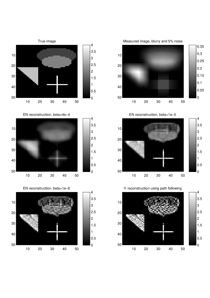
Figure 2: A true image and its blurry and noisy measurement together with elastic-net reconstructions for $\alpha=1\times 10^{-4}$ and different values of $\beta$ and the $\ell^{1}$-reconstruction.

5 Conclusion

We analyzed the elastic-net regularization from an “inverse problem” point of view. Using classical and modern techniques we showed that elastic-net regularization combines the best of both $\ell^{2}$- and $\ell^{1}$-regularization, i.e. the good convergence rate of $\ell^{1}$-regularization and modest constants in the error estimates from $\ell^{2}$-regularization. Moreover, we also showed that the a posteriori parameter choice due to Morozov also works for elastic-net regularization and leads to the same convergence rates as our a priori choice. Large parts of our analysis were based on a linear coupling of the two regularization parameters. However, Theorem 2.7 indicates that an asymptotic linear coupling of the parameters would suffice. From Example 2.8 one may conjecture that there is a critical value of the coupling constant $\eta$ for all values greater than which the minimal-$\eta\|\cdot\|_{\ell^{1}}+\tfrac{1}{2}\|\cdot\|_{\ell^{2}}^{2}$-solution coincides with the minimal-$\|\cdot\|_{\ell^{1}}$-solution. This would provide a further justification for the elastic-net functional.

We have also developed two active set methods for minimizing the elastic-net functional and numerically confirmed their excellent performance. We may state that elastic-net is coequal to classical $\ell^{1}$ minimization in terms of relative error, sparsity and computation time for well conditioned problems and is favorably for ill-conditioned problems.

References

- [1] H. Attouch, G. Buttazo, and G. Michaille. Variational Analysis in Sobolev and Spaces: Applications to PDEs and Optimization. SIAM, Philadelphia, 2006.
- [2] Thomas Bonesky. Morozov’s discrepancy principle and Tikhonov-type functionals. Inverse Problems, 25(1):015015, 2009.
- [3] Kristian Bredies and Dirk A. Lorenz. Iterated hard shrinkage for minimization problems with sparsity constraints. SIAM Journal on Scientific Computing, 30(2):657–683, 2008.
- [4] Kristian Bredies and Dirk A. Lorenz. Linear convergence of iterative soft-thresholding. Journal of Fourier Analysis and Applications, 14(5–6):813–837, 2008.
- [5] Martin Burger and Stanley Osher. Convergence rates of convex variational regularization. Inverse Problems, 20(5):1411–1420, 2004.
- [6] Emmanuel J. Candés and Terrence C. Tao. Near optimal signal recovery from random projections: universal encoding strategies. IEEE Transactions on Information Theory, 52(1):5406–5425, 2006.
- [7] Scott Shaobing Chen, David L. Donoho, and Michael A. Saunders. Atomic decomposition by basis pursuit. SIAM Journal on Scientific Computing, 20(1):33–61, 1998.
- [8] Xiaojun Chen, Zuhair Nashed, and Liqun Qi. Smoothing methods and semismooth methods for nondifferentiable operator equations. SIAM Journal on Numerical Analysis, 38(4):1200–1216, 2000.
- [9] Ingrid Daubechies, Michel Defrise, and Christine De Mol. An iterative thresholding algorithm for linear inverse problems with a sparsity constraint. Communications in Pure and Applied Mathematics, 57(11):1413–1457, 2004.
- [10] C. De Mol, E. De Vito, and L. Rosasco. Elastic-net regularization in learning theory. Journal of Complexity, 25(2):201–230, 2009.
- [11] Heinz W. Engl, Martin Hanke, and Andreas Neubauer. Regularization of Inverse Problems, volume 375 of Mathematics and its Applications. Kluwer Academic Publishers Group, Dordrecht, 2000.
- [12] Mário A. T. Figueiredo and Robert D. Nowak. An EM algorithm for wavelet-based image restoration. IEEE Transactions on Image Processing, 12(8):906–916, 2003.
- [13] Mário A. T. Figueiredo, Robert D. Nowak, and Stephen J. Wright. Gradient projection for sparse reconstruction: Applications to compressed sensing and other inverse problems. IEEE Journal of Selected Topics in Signal Processing, 1(4):586–597, 2007.
- [14] Markus Grasmair, Markus Haltmeier, and Otmar Scherzer. Sparse regularization with penalty term. Inverse Problems, 24(5):055020 (13pp), 2008.
- [15] Roland Griesse and Dirk A. Lorenz. A semismooth Newton method for Tikhonov functionals with sparsity constraints. Inverse Problems, 24(3):035007 (19pp), 2008.
- [16] Elaine T. Hale, Wotao Yin, and Yin Zhang. Fixed-point continuation for l1-minimization: Methodology and convergence. SIAM J. Optim., 19(3):1107–1130, 2008.
- [17] Per Christian Hansen. Regularization Tools Version 4.0 for Matlab 7.3. Numerical Algorithms, 46:189–194, 2007.
- [18] Michael Hintermüller, Kazufumi Ito, and Karl Kunisch. The primal-dual active set strategy as a semismooth Newton method. SIAM Journal on Optimization, 13(3):865–888, 2003.
- [19] K. Ito and K. Kunisch. On the choice of the regularization parameter in nonlinear inverse problems. SIAM Journal on Optimization, 2(3):376–404, 1992.
- [20] Bangti Jin and Jun Zou. Iterative schemes for Morozov’s discrepancy principle in optimizations arising from inverse problems. submitted, 2009.
- [21] Honglak Lee, Alexis Battle, Rajat Raina, and Andrew Y. Ng. Efficient sparse coding algorithms. In B. Schölkopf, J. Platt, and T. Hoffman, editors, Advances in Neural Information Processing Systems 19, pages 801–808. MIT Press, Cambridge, MA, 2007.
- [22] S. Levy and P. Fullager. Reconstruction of a sparse spike train from a portion of its spectrum and application to high-resolution deconvolution. Geophysics, 46(9):1235–1243, 1981.
- [23] Dirk A. Lorenz. Convergence rates and source conditions for Tikhonov regularization with sparsity constraints. Journal of Inverse and Ill-Posed Problems, 16(5):463–478, 2008.
- [24] Ignace Loris. On the performance of algorithms for the minimization of -penalized functionals. Inverse Problems, 25(3):035008, 2009.
- [25] R. Tyrrell Rockafellar. Convex Analysis. Princeton University Press, Princeton, 1970.
- [26] H. Taylor, S. Bank, and J. McCoy. Deconvolution with the norm. Geophysics, 44(1):39–52, 1979.
- [27] R. Tibshirani. Regression shrinkage and selection via the lasso. Journal of the Royal Statistical Society, Series B, 58(1):267–288, 1996.
- [28] S. Ulbrich. Semismooth newton methods for operator equations in function spaces. SIAM Journal on Optimization, 13(3):805–842, 2002.
- [29] S. J. Wright, R. D. Nowak, and M. A. T. Figueiredo. Sparse reconstruction by separable aproximation. IEEE Transactions on Signal Processing, 57(7):2479–2493, 2009.
- [30] Hui Zou and Trevor Hastie. Regularization and variable selection via the elastic net. Journal of the Royal Statistical Society, Series B, 67(2):301–320, 2005.