The Refractive Index of Curved Spacetime II:
QED, Penrose Limits and Black Holes

Abstract:

This work considers the way that quantum loop effects modify the propagation of light in curved space. The calculation of the refractive index for scalar QED is reviewed and then extended for the first time to QED with spinor particles in the loop. It is shown how, in both cases, the low frequency phase velocity can be greater than $c$, as found originally by Drummond and Hathrell, but causality is respected in the sense that retarded Green functions vanish outside the lightcone. A “phenomenology” of the refractive index is then presented for black holes, FRW universes and gravitational waves. In some cases, some of the polarization states propagate with a refractive index having a negative imaginary part indicating a potential breakdown of the optical theorem in curved space and possible instabilities.

1 Introduction

The quantum theory of photon propagation in curved spacetime raises many challenging questions, particularly in relation to the realization of causality and unitarity in quantum field theories with a fixed gravitational background. In particular, in previous work [4, 3, 2] we have shown that vacuum polarization effects in curved spacetime lead to the phenomenon that curved spacetime acts like an optical medium and can be described by means of a refractive index. However, this index has a novel analytic structure, compared with conventional optical media, and standard formulae, notably the Kramers-Kronig dispersion relation are violated. This analytic structure has an origin in the geometry of null geodesic congruences and their conjugate points which give rise to curved-spacetime-specific singularities in the Van Vleck-Morette determinant and consequently the Green functions.

This line of research began with the apparent paradox of how to reconcile the requirements of causality with the observation by Drummond and Hathrell [5] that at low frequencies the phase velocity of light in a gravitational background can be superluminal (i.e. the refractive index $n(\omega)<1$ for $\omega$ small). Since causality plays such an important rôle in the theory, it is worthwhile stating exactly what is meant in the context of a QFT. Causality in this context is often called “micro-causality”, and is the property that the retarded/advanced Green functions only have non-vanishing support inside (or on) the backward/forward lightcone. The requirement of causality can be linked directly to the refractive index itself [2] leading to two conditions: (i) $n(\omega)\to 1$ for large $|\omega|$; and (ii) $n(\omega)$ must be an analytic function in the upper-half of the complex $\omega$ plane. The first condition is equivalent to the requirement that the wavefront velocity, the high frequency limit of the phase velocity, is equal to $c$ [6, 7]. Notice that neither of these conditions could be tested in the original work of Drummond and Hathrell which was restricted to small $\omega$. However, prior to the unlocking of the full frequency-dependence of $n(\omega)$ in [2, 3, 4], the following argument led to a paradox. In conventional dispersive, or dielectric, media the refractive index obeys the familiar Kramers-Kronig dispersion relation

$$n(\infty)~{}~{}=~{}~{}n(0)~{}-~{}\int_{0}^{\infty}{d\omega\over\omega}~{}\operatorname{Im}~{}n(\omega)\ .$$ (1)

Since $\operatorname{Im}n(\omega)$ is constrained to be positive, being related by the optical theorem (itself a consequence of unitarity) to a forward scattering cross-section, eq.(1) implies $n(\infty)<n(0)$. This would mean a superluminal low frequency refractive index $n(0)<1$ would be incompatible with a causal limit $n(\infty)=1$. The resolution, found in refs.[2, 3, 4], is that spacetime behaves like an optical medium for which the Kramers-Kronig relation no longer holds in the form (1) and, furthermore, $\operatorname{Im}n(\omega)$ is not constrained to be positive. One can trace this non-compliance to the novel analytic structure—compared with conventional dielectric media—of the refractive index of curved spacetime.

In curved spacetime, the refractive index will in general be a local quantity $n(x,\omega)$, since spacetime is not generally homogeneous, (as well as a matrix quantity in order to describe the two polarization states of the photon). What we will find is that $n(x,\omega)$ is consistent with micro-causality, as a consequence of analyticity in the upper-half $\omega$ plane, and consequently one can write a version of the Kramers-Kronig relation in the form

$$n(x,\infty)~{}~{}=~{}~{}n(x,0)~{}-~{}{1\over{i\pi}}{\cal P}\int_{-\infty}^{\infty}{d\omega\over\omega}~{}n(x,\omega)\ ,$$ (2)

which does hold. The usual relations that hold in models of dispersive media, namely the fact that $n(\omega)$ is an even function of $\omega$ and the property of hermitian analyticity, $n(\omega-i\epsilon)=n(\omega+i\epsilon)^{*}$, which together imply that $n(\omega+i\epsilon)=n(-\omega+i\epsilon)^{*}$, then lead to (1). Neither of these relations hold in curved spacetime which, as we shall see, allows the causality constraint $n(x,\infty)=1$ to hold even in the presence of a superluminal $n(x,0)<1$.

Although this resolution of causality with a low-frequency superluminal phase velocity is achieved through the modification of the Kramers-Kronig relation to accommodate the novel analytic structure of $n(x,\omega)$ in curved spacetime, in the course of studying particular examples in refs.[2, 3, 4] we found cases where $\operatorname{Im}n(x,\omega)$ is in fact negative. This is unexpected since one would have expected this imaginary part to signal the decay of the photon into real $e^{+}e^{-}$ pairs and hence be strictly positive: it appears that the optical theorem cannot hold—at least in its conventional form—in curved spacetime [8]. The correct interpretation of a negative imaginary part, the fate of the optical theorem and implication that the photon modes have an increasing amplitude, will be left to future work; one of the purposes of the present paper is to collect the “phenomenological” evidence on this issue by studying several relevant spacetimes.

In order to establish these results, we calculated the complete frequency dependence of the refractive index for scalar QED, obtaining a concise formula involving the Van Vleck-Morette (VVM) matrix [2]. This makes clear the geometric origin of the final result, and therefore its generality: loop corrections to Green functions in curved spacetime will generically have a richer analytic structure than in flat spacetime. The quantum corrections to photon propagation are governed by the one-loop vacuum polarization. As shown in refs.[4, 3, 2], both in a worldline formalism and using the more conventional heat kernel (or proper time) formalism, when the mass of the electron is much greater than the curvature scale and so the “geodesic approximation” applies, this is determined by a path integral over fluctuations around the classical null geodesic traced by the photon; in turn, these are governed by the geometry of geodesic deviation, explaining the origin of the VVM matrix in the final result. The great simplification is that to leading order in a weak curvature expansion, the geometry of geodesic deviation is entirely encoded in the Penrose limit [9] of the original spacetime around the photon’s classical null trajectory. It follows that the whole problem of determining the refractive index can be resolved simply by studying the appropriate Penrose plane wave limit, with all the relevant information on the background spacetime being encoded in the plane wave profile function $h_{ij}(u)$ to be defined in due course.

In this paper, we develop these fundamental ideas in a number of directions, in effect building up a phenomenology of the interesting and counter-intuitive effects that can arise in what we have previously termed “quantum gravitational optics” [10]. We begin by reviewing and simplifying the conceptual basis of our calculation of the refractive index for scalar QED in curved spacetime, highlighting the rôle played by the Penrose limit in determining the vacuum polarization and the relation of the geometry of null geodesic congruences to the analytic structure of the refractive index. Next we calculate the refractive index for spinor QED, introducing the necessary geometric tools, in particular the spinor parallel transporter in a plane wave spacetime, and evaluating the vacuum polarization for a massive spinor loop. The result is qualitatively similar to the simpler case of scalar QED and displays the same generic analyticity properties, but also shows some physically interesting differences in particular models.

We then consider photon propagation in a variety of examples of gravitational backgrounds in order to build up intuition about the rôle of symmetries, singularities and time-dependence of the curved spacetime in the realization of causality and unitarity in QED. In each case, we need to find the Penrose limit corresponding to the classical photon trajectory of interest, then solve the geodesic deviation equations to construct the VVM matrix from which the vacuum polarization and refractive index follow. In most cases, we have to resort to a numerical evaluation of the refractive index itself.

The first examples are homogeneous plane waves. These are interesting both as simple toy models and as the Penrose limits of certain geodesics in classical black hole and cosmological spacetimes near the singularity. They have a large spacetime isometry group, an extension of the Heisenberg algebra, and can be usefully realized as coset spaces. We consider two cases, the symmetric plane waves originally studied in refs.[2, 3, 4] and the singular homogeneous plane waves which arise as near-singularity Penrose limits. The next set of backgrounds that are considered are the black hole spacetimes, especially the Schwarzschild and Kerr metrics. These are examples of Petrov type D spacetimes and we can exploit the resulting simplifications to give a very general description of the Penrose limits for various choices of geodesics. In particular, the Penrose limit corresponding to the principal null geodesics are flat, implying that the quantum corrections to the refractive index vanish identically, a result already observed in the low-frequency limit. We also see how in general the Penrose plane wave profile depends on the Walker-Penrose integral of motion [11, 12] characterizing the classical trajectory and show how the near-singularity limits reduce to singular homogeneous plane waves in the Penrose limit.

We then go on to consider FRW universes. In these spaces the definition of the refractive index needs a slight modification because the singularity in the past does not allow one to consider waves coming in from past null infinity. Finally, we discuss the behaviour of the refractive index in both a weak gravitational wave and a gravitational shockwave.

2 Vacuum polarization and Photon Propagation in Curved Spacetime

We begin by reviewing briefly the eikonal formalism and the derivation of the refractive index in the low-frequency effective action from the QED effective action [2].

In classical electrodynamics, the propagation of photons in curved spacetime is governed by the Maxwell equation $\nabla_{\mu}F^{\mu\nu}=0$, with $F_{\mu\nu}=\nabla_{\mu}A_{\nu}-\nabla_{\nu}A_{\mu}$. In the eikonal approximation, the electromagnetic field is written in terms of a slowly-varying (with respect to the curvature scale) amplitude ${\cal A}(x)$ and a rapidly-varying phase $\Theta(x)$ as follows:

$$A_{\mu}(x)={\cal A}(x)\hat{\varepsilon}_{\mu}(x)e^{i\Theta(x)}\ ,$$ (3)

where $\hat{\varepsilon}_{\mu}(x)$ is the polarization tensor. The wave-vector is identified as $k_{\mu}=\partial_{\mu}\Theta$ and we fix the gauge so that the two independent polarizations $\hat{\varepsilon}_{(i)}$, $i=1,2$ satisfy the transverse condition $k\cdot\hat{\varepsilon}_{(i)}=0$, have vanishing component along $k^{\mu}$ and are spacelike normalized such that $\hat{\varepsilon}_{(i)}\cdot\hat{\varepsilon}_{(j)}=\delta_{ij}$. The eikonal expansion is in powers of the frequency $\omega$ and is valid in the regime $\omega\gg\sqrt{R}$, with $R$ a typical curvature scale. The wave vector itself is ${\cal O}(\omega)$ whereas ${\cal A}$ and $\hat{\varepsilon}_{\mu}$ are ${\cal O}(1)$, so at leading order, the Maxwell equation gives

$$k^{2}=\partial\Theta\cdot\partial\Theta=0\ .$$ (4)

Since this also implies $k\cdot\nabla k^{\mu}=0$, it follows that the integral curves of the vector field $k^{\mu}$ are null geodesics, which are identified as the classical trajectories of the photon. At next-to-leading order, the eikonal equations describe the variation of the amplitude and polarization along these null geodesics:

$$\begin{split}k\cdot\nabla\,\hat{\varepsilon}^{\mu}&=0\ ,\\ k\cdot\nabla\,\log{\cal A}&=-\tfrac{1}{2}\nabla\cdot k\ .\end{split}$$ (5)

The second of these relates the change in amplitude to the expansion $\hat{\theta}\equiv\nabla_{\mu}\hat{k}^{\mu}$ (with $\hat{k}^{\mu}=\omega^{-1}k^{\mu}$), one of the optical scalars in the Raychaudhuri equations.

In order to study photon propagation in a general spacetime, it is convenient to use a set of coordinates that are specially adapted to the vector field $k^{\mu}$. These are the Penrose coordinates, which are also known as “adapted coordinates”, $(u,V,Y^{a})$, $a=1,2$. Here, $u$ is the affine parameter along a null geodesic, $V$ is the associated null coordinate and $Y^{a}$ are two orthogonal spacelike coordinates. This choice corresponds to the embedding of the preferred null geodesic $\gamma$ (with $V=Y^{a}=0$), representing the classical photon trajectory, in a twist-free null congruence labelled by constant $V,Y^{a}$. The metric $g_{\mu\nu}$ can always be written in terms of these adapted coordinates in the form [13]:

$$ds^{2}=-2du\,dV+C(u,V,Y^{a})dV^{2}+2C_{a}(u,V,Y^{b})dY^{a}\,dV+C_{ab}(u,V,Y^{c})dY^{a}\,dY^{b}\ .$$ (6)

The eikonal phase is then taken to be $\Theta=-\omega V$, the Fourier mode appropriate for a metric with an isometry characterized by a Killing vector $\partial_{V}$, so that $\hat{k}^{\mu}=(1,0,0,0)$. In terms of these coordinates the transport equations (5) are

$$\begin{split}\nabla_{u}\hat{\varepsilon}^{\mu}=0\ ,\\ \partial_{u}\log{\cal A}=-\tfrac{1}{2}\hat{\theta}\ ,\end{split}$$ (7)

where the expansion scalar is

$$\hat{\theta}=\tfrac{1}{2}C^{ab}\partial_{u}C_{ab}=\partial_{u}\log\sqrt{g}\ ,$$ (8)

where $C^{ab}$ denotes the inverse of $C_{ab}$ and $g=-{\rm det}g_{\mu\nu}$.

Going beyond the classical theory and including the effects of vacuum polarization, the Maxwell equation is replaced by

$$\nabla_{\nu}F^{\nu}{}_{\mu}~{}=~{}4\int\sqrt{g(x^{\prime})}\,d^{4}x^{\prime}\,\Pi^{\text{1-loop}}_{\mu\nu}(x,x^{\prime})A^{\nu}(x^{\prime})\ .$$ (9)

where $\Pi_{\mu\nu}^{\text{1-loop}}(x,x^{\prime})$ is the vacuum polarization tensor appearing in the one-loop effective action

$$\Gamma^{\text{1-loop}}~{}=~{}-\int\sqrt{g(x)}\,d^{4}x\,\sqrt{g(x^{\prime})}d^{4}x^{\prime}\,A^{\mu}(x)\Pi^{\text{1-loop}}_{\mu\nu}(x,x^{\prime})A^{\nu}(x^{\prime})\ .$$ (10)

In general, we find that the wave vector is no longer null and the physical light cone defined by $k^{2}$ no longer coincides with the geometric null cones. In physical terms, the phase velocity of light is no longer necessarily $c$ and may be either sub- or super-luminal [5]. It can also become polarization dependent, i.e. display gravitationally induced bi-refringence.

To accommodate this, we modify the eikonal phase as follows:

$$\Theta=-\omega\big{(}V\delta_{ij}-\vartheta_{ij}(x;\omega)\big{)}\ .$$ (11)

where we now think of the phase as a $2\times 2$ matrix with respect to the polarizations $\hat{\varepsilon}_{(i)}$. With this form for the electromagnetic field $A_{\mu}(x)$, and using the metric (6), we find

$$\nabla_{\mu}F_{(i)}^{\mu\nu}=2\omega^{2}\frac{\partial\vartheta_{ij}(x;\omega)}{\partial u}{\cal A}\hat{\varepsilon}_{(j)}^{\nu}e^{-i\omega V}\ ,$$ (12)

to leading order in the eikonal expansion. Provided $\vartheta_{ij}(x)$ is perturbatively small, i.e. ${\cal O}(\alpha)$, this corresponds to a refractive index matrix:

$$\boldsymbol{n}(x;\omega)=\boldsymbol{1}+\frac{\partial\boldsymbol{\vartheta}(x;\omega)}{\partial u}\ .$$ (13)

The phase $\boldsymbol{\vartheta}(x;\omega)$ is then determined from the leading, ${\cal O}(\omega^{2})$ piece of the r.h.s. of (12) evaluated with the eikonal ansatz (3),(11) for $A_{\mu}(x)$. Putting all this together, we find the following compact expression for the refractive index:

$$n_{ij}(x;\omega)~{}=~{}\delta_{ij}-\frac{2}{\omega^{2}}\int dx^{\prime}\sqrt{g(x^{\prime})}~{}{{\cal A}(x^{\prime})\over{\cal A}(x)}~{}\hat{\varepsilon}_{(i)}^{\mu}(x)~{}\Pi^{\text{1-loop}}_{\mu\nu}(x,x^{\prime})~{}\hat{\varepsilon}_{(j)}^{\nu}(x^{\prime})~{}e^{i\omega(V-V^{\prime})}\ .$$ (14)

The polarizations which propagate with well-defined phase velocities are the linear combinations of the basis $\hat{\varepsilon}_{(i)}$ giving the eigenstates of $\boldsymbol{n}$.

To see how this works in the simplest case, we consider first the low-frequency limit of the refractive index, which exhibits superluminal phase velocities. This can be found by considering the modifications to the Maxwell equation following from the leading terms in a derivative expansion of the one-loop effective action and was the approach taken in the original work of Drummond and Hathrell [5]. The relevant terms in the low-frequency effective action to one loop are

$$\begin{split}\Gamma~{}~{}=~{}\int d^{4}x\,\sqrt{g}\Big{[}&-\frac{1}{4}ZF_{\mu\nu}F^{\mu\nu}~{}+~{}d\nabla_{\mu}F^{\mu\lambda}\nabla_{\nu}F^{\nu}{}_{\lambda}\\ &+~{}aRF_{\mu\nu}F^{\mu\nu}~{}+~{}bR_{\mu\nu}F^{\mu\lambda}F^{\nu}{}_{\lambda}~{}+~{}cR_{\mu\nu\lambda\rho}F^{\mu\nu}F^{\lambda\rho}~{}~{}\Big{]}\ ,\end{split}$$ (15)

where the coefficients for both scalar and spinor QED can be read off from [14] and are given in [2]. We find

$$a=0\ ,~{}~{}~{}~{}~{}~{}b=-\frac{\alpha}{720\pi m^{2}}\ ,~{}~{}~{}~{}~{}~{}c=-\frac{\alpha}{1440\pi m^{2}}\ ,~{}~{}~{}~{}~{}~{}d=\frac{\alpha}{480\pi m^{2}}\ ,$$ (16)

for scalar QED, while

$$a=-\frac{\alpha}{144\pi m^{2}}\ ,~{}~{}~{}~{}~{}~{}b=\frac{13\alpha}{360\pi m^{2}}\ ,~{}~{}~{}~{}~{}~{}c=-\frac{\alpha}{360\pi m^{2}}\ ,~{}~{}~{}~{}~{}~{}d=-\frac{\alpha}{30\pi m^{2}}\ ,$$ (17)

for spinor QED, reproducing the original Drummond-Hathrell effective action [5]. $Z=1+\tfrac{\alpha}{6\pi}\log{m^{2}\over\mu^{2}}$ is the one-loop wave-function renormalization factor.

To find the refractive index, we first evaluate the vacuum polarization tensor from (15). Since this effective action is local, $\Pi^{\text{1-loop}}(x,x^{\prime})$ is proportional to $\delta(x,x^{\prime})$ and (14) simplifies immediately since, for example, the amplitude factors cancel and the polarizations are evaluated at the same point. This immediately gives the general result for the low-frequency limit of the refractive index [5, 10]

$$n_{ij}^{\text{spinor}}(0)=\delta_{ij}-2bR_{uu}\delta_{ij}-8cR_{uiuj}\ .$$ (18)

where $R_{uiuj}\equiv R_{u\lambda u\rho}\hat{\varepsilon}_{(i)}^{\lambda}\hat{\varepsilon}_{(j)}^{\rho}$. So for scalar QED we find

$$n_{ij}^{\text{scalar}}(0)=\delta_{ij}-\frac{\alpha}{360\pi m^{2}}\big{(}R_{uu}\delta_{ij}+2R_{uiuj}\big{)}\ ,$$ (19)

while for spinor QED,

$$n_{ij}^{\text{spinor}}(0)=\delta_{ij}-\frac{\alpha}{180\pi m^{2}}\big{(}13R_{uu}\delta_{ij}-4R_{uiuj}\big{)}\ ,$$ (20)

The generalization of the QED effective action to all orders in derivatives was found in ref.[14, 15] and can be used to extend the expression (18) for the refractive index $n_{ij}(0)$ to a full perturbative expansion of $n_{ij}(\omega)$ in powers of $\omega$. This effective action consists of “$RFF$” operators acted on by functions of the Laplacian, viz.

$$\begin{split}\Gamma~{}=~{}&\int d^{4}x\sqrt{-g}~{}\biggl{[}-{1\over 4}ZF_{\mu\nu}F^{\mu\nu}~{}+~{}\nabla_{\mu}F^{\mu\lambda}\overrightarrow{d_{0}}\nabla_{\nu}F^{\nu}{}_{\lambda}\\ &+~{}{1\over m^{2}}\Bigl{(}\overrightarrow{a_{0}}RF_{\mu\nu}F^{\mu\nu}~{}+~{}\overrightarrow{b_{0}}R_{\mu\nu}F^{\mu\lambda}F^{\nu}{}_{\lambda}~{}+~{}\overrightarrow{c_{0}}R_{\mu\nu\lambda\rho}F^{\mu\nu}F^{\lambda\rho}\Bigr{)}\\ &+~{}{1\over m^{4}}\Bigl{(}\overrightarrow{a_{1}}R\nabla_{\mu}F^{\mu\lambda}\nabla_{\nu}F^{\nu}{}_{\lambda}~{}+~{}\overrightarrow{b_{1}}R_{\mu\nu}\nabla_{\lambda}F^{\lambda\mu}\nabla_{\rho}F^{\rho\nu}\\ &+~{}\overrightarrow{b_{2}}R_{\mu\nu}\nabla^{\mu}F^{\lambda\rho}\nabla^{\nu}F_{\lambda\rho}~{}+~{}\overrightarrow{b_{3}}R_{\mu\nu}\nabla^{\mu}\nabla^{\lambda}F_{\lambda\rho}F^{\rho\nu}~{}+~{}\overrightarrow{c_{1}}R_{\mu\nu\lambda\rho}\nabla_{\sigma}F^{\sigma\rho}\nabla^{\lambda}F^{\mu\nu}~{}\Bigr{)}\biggr{]}\end{split}$$ (21)

In this formula, the $\overrightarrow{a_{n}}$, $\overrightarrow{b_{n}}$, $\overrightarrow{c_{n}}$ are known “form factor” functions of three operators, i.e.

$$\overrightarrow{a_{n}}\equiv a_{n}\Bigl{(}{\nabla_{(1)}^{2}\over m^{2}},{\nabla_{(2)}^{2}\over m^{2}},{\nabla_{(3)}^{2}\over m^{2}}\Bigr{)}\ ,$$ (22)

where the first entry $\nabla_{(1)}^{2}/m^{2}$ acts on the first following term (the curvature), etc. The form factors can be extracted from the very general background field effective action originally computed by Barvinsky et al. [16] and are described in detail in ref.[14, 15].

Extracting the refractive index from (21) to leading order in the eikonal approximation involves a number of subtleties, which are discussed in detail in ref.[15]. The result is an expression of the form

$$n_{ij}(\omega)~{}=~{}\delta_{ij}~{}+~{}\delta_{ij}B\Bigl{(}{2i\omega{\hat{k}}\cdot\nabla\over m^{2}}\Bigr{)}\frac{R_{uu}}{m^{2}}~{}+~{}C\Bigl{(}{2i\omega{\hat{k}}\cdot\nabla\over m^{2}}\Bigr{)}\frac{R_{uiuj}}{m^{2}}\ ,$$ (23)

where the constant coefficients are replaced by functions of the operator ${\hat{k}}\cdot\nabla$, which describes the variation of the curvature tensors along the original null geodesic $\gamma$. Since $B(x)$ and $C(x)$ are real functions it follows immediately that even perturbatively at ${\cal O}(\omega)$, a non-constant curvature along $\gamma$ will give rise to an imaginary part of the refractive index, which can be positive or negative depending on the variation of the curvature along the geodesic.

The expression above (23), captures all the terms which are linear in the curvature. In the present work, we will calculate an expression for the refractive index whose scope is much wider because its sums up all powers of the curvature (as well as its derivatives). The only assumptions are that the curvature is weak, in the sense that $R\ll m^{2}$, and the eikonal approximation is valid $\omega\gg\sqrt{R}$. Schematically we find

$$n_{ij}(\omega)=\delta_{ij}+\frac{\alpha R}{m^{2}}F_{ij}\left(\frac{\omega\sqrt{R}}{m^{2}}\right)\ ,$$ (24)

where $R$ is a generic curvature scale.

To find the full frequency dependence of the refractive index, therefore, we need to find the exact form of the vacuum polarization $\Pi^{\text{1-loop}}_{\mu\nu}$ acting on the eikonal ansatz for the electromagnetic field. Even the complete expansion of the effective action to all-orders in derivatives is not sufficient to capture the non-perturbative behaviour of $n_{ij}(\omega)$ as a function of frequency [3, 4, 15]. This was achieved in refs.[3, 4], in a calculation based on the worldline approach to QFT, and subsequently in [2] using the more conventional heat kernel, or proper time, representation of the propagators.

The key insight in both these methods is that when $R\ll m^{2}$ we can use the “geodesic approximation” for the the propagators of the electron and positron in the loop. When the loop is coupled to an external photon the geodesic approximation leads to a simple picture: the electron and positron follow the original geodesic of the photon before annihilating back into the photon. Therefore the vacuum polarization is determined by the geometry of geodesic fluctuations about the photon’s classical trajectory and hence to leading order in “weak” curvature, i.e. ${\cal O}(R/m^{2})$, the refractive index is governed entirely by the Penrose limit of the original curved spacetime. This is because the Penrose limit is a truncation of the original spacetime metric which captures the tidal forces corresponding to geodesic deviation. Since the Penrose limit describes a plane wave metric, we find the remarkable simplification that at weak curvature, the refractive index for any given spacetime may be calculated simply by considering propagation in the associated plane wave background.

We explain in detail how this comes about in Section 4, where we re-cap the essential points of the derivation of the refractive index for scalar QED [2]. First, we discuss the most important aspects of the Penrose limit, plane wave spacetimes, geodesic deviation and the Van Vleck-Morette determinant from the perspective of photon propagation in curved spacetime.

3 Penrose limit and Geometry of Plane Wave Spacetimes

In this section, we collect the essential results about the geometry of the Penrose limit [9] and plane waves which will be used in the QFT calculations later in the paper. For further details and discussion, see the reviews in refs.[2] and [13].

3.1 Geodesic deviation and the optical tensors

Before introducing the Penrose limit, we describe the basic geometry of geodesic deviation in the context of the general metric (6) in coordinates adapted to the null congruence around $\gamma$. We therefore consider the connecting vector $z^{\mu}$ which connects corresponding points on neighbouring geodesics in the congruence and study its evolution along $\gamma$. This is determined by the requirement that the Lie derivative of $z^{\mu}$ along $\gamma$ vanishes, i.e.

$${\cal L}_{\hat{k}}z^{\mu}~{}\equiv~{}\hat{k}\cdot\nabla z^{\mu}-(\nabla_{\nu}\hat{k}^{\mu})z^{\nu}~{}=~{}0\ .$$ (25)

This implies

$$\nabla_{u}z^{\mu}~{}=~{}\Omega^{\mu}{}_{\nu}z^{\nu}\ ,$$ (26)

where $\Omega_{\mu\nu}=\nabla_{\mu}\hat{k}_{\nu}$, which plays the role of a connection for the Lie derivative, is symmetric since the vector field $\hat{k}^{\mu}$ is a gradient flow.

To describe geodesic flow and the Raychaudhuri equations, it is sufficient to consider connecting vectors with transverse components $z^{a}$ only. In the Penrose coordinates (6), we have

$$\nabla_{u}z^{a}~{}=~{}\Omega^{a}{}_{b}z^{b}\ ,$$ (27)

with

$$\Omega_{ab}=\frac{1}{2}\partial_{u}C_{ab}\ ,$$ (28)

It follows from (27) that the transverse components of the connecting vector satisfy the geodesic deviation equation:

$$\nabla_{u}\nabla_{u}z^{a}~{}=~{}-R^{a}{}_{ubu}z^{b}~{}\equiv~{}-h^{a}{}_{b}z^{b}\ ,$$ (29)

where

$$h^{a}{}_{b}~{}=~{}-\nabla_{u}\Omega^{a}{}_{b}-\Omega^{a}{}_{c}\Omega^{c}{}_{b}\ ,\\$$ (30)

that is,

$$R_{aubu}~{}=~{}-\frac{1}{2}\partial_{u}^{2}C_{ab}~{}+~{}\frac{1}{4}\partial_{u}C_{ac}~{}C^{cd}~{}\partial_{u}C_{db}\ .$$ (31)

A solution $z^{a}$ of (29) is known as a “Jacobi field” on the null geodesic $\gamma$.

The important point here is that the transverse geodesic fluctuations are controlled entirely by the metric components $C_{ab}$ in (6). As we see below, this underlies the key rôle to be played by the Penrose limit.

The nature of the geodesic flow is most elegantly summarized in the Raychaudhuri equations for the optical tensors. These are defined from $\Omega_{ab}$ as:

$$\Omega_{ab}~{}=~{}\frac{1}{2}\hat{\theta}C_{ab}+\hat{\sigma}_{ab}+\hat{\omega}_{ab}\ ,$$ (32)

where $\hat{\theta}$, $\hat{\sigma}_{ab}$, $\hat{\omega}_{ab}$ are respectively the expansion, shear and twist of the null congruence. Here, the twist is vanishing by construction, since $\hat{k}^{\mu}$ is by definition a gradient field, and for this reason (6) embeds the geodesic $\gamma$ in a twist-free null congruence.

The Raychaudhuri equations are equivalent to (30), which reads

$$\nabla_{u}\Omega_{ab}~{}=~{}-\Omega_{ac}C^{cd}\Omega_{db}~{}-~{}R_{aubu}\ .$$ (33)

In terms of the optical scalars:

$$\begin{split}\partial_{u}\hat{\theta}~{}&=~{}-\tfrac{1}{2}\hat{\theta}^{2}-\hat{\sigma}_{ab}\hat{\sigma}^{ab}-R_{uu}\ ,\\ \nabla_{u}\hat{\sigma}_{ab}~{}&=~{}-\hat{\theta}\hat{\sigma}_{ab}-{\cal C}_{aubu}\,\end{split}$$ (34)

where the Weyl tensor ${\cal C}_{aubu}$ is the trace-free part of the Riemann tensor (31).

Notice that the equation for the expansion immediately shows that $\partial_{u}\hat{\theta}\leq 0$ everywhere along the geodesic provided the null energy condition $R_{uu}>0$ holds, implying a generic focusing of the null congruence. Moreover, if we define the shear scalar as $\hat{\sigma}=\sqrt{2}\hat{\sigma}_{ab}\hat{\sigma}^{ab}$ and introduce Newman-Penrose scalars $\Phi_{00}=\tfrac{1}{2}R_{uu}$ and (in a null basis $m^{\mu},\bar{m}^{\mu}$ for the transverse directions aligned with the eigenvalues of $\sigma_{ab}$) $\Psi_{0}={\cal C}_{umum}$, we can write the Raychaudhuri equations as

$$\partial_{u}(\hat{\theta}\pm\hat{\sigma})~{}=~{}-\tfrac{1}{2}(\hat{\theta}\pm\hat{\sigma})^{2}-2(\Phi_{00}\mp\Psi_{0})\ .$$ (35)

Physically, this shows that at a given point along the geodesic $\gamma$, the congruence must be focusing in at least one of the transverse directions. While locally, focus/focus and focus/defocus are permitted, the null energy condition prohibits a congruence with defocus/defocus.

This illustrates a crucial theorem [17], that for a spacetime satisfying the “null generic condition” ($\Phi_{00}\neq 0$ or $\Psi_{0}\neq 0$ at some point) and the null energy condition, every complete null geodesic possesses a pair of conjugate points. Two points $p$ and $q$ on a null geodesic are said to be conjugate if there exists a Jacobi field $z^{a}\in\hat{\cal V}$ which is not identically zero but which vanishes at both $p$ and $q$. Loosely speaking, this implies there is an “infinitesimally deformed” null geodesic intersecting $\gamma$ at both $p$ and $q$. As we see in the next section, this is precisely the property of geodesic fluctuations which is reflected in the quantum field theory. Notice though that this definition of conjugate points is linked to infinitesimal deviations and does not necessarily lift to geodesics of the full metric; in particular, the existence of conjugate points $p$ and $q$ does not imply that there is an actual geodesic, other than $\gamma$, joining $p$ and $q$.

Another important set of coordinates, specifically designed to study fluctuations around a given null geodesic, are null Fermi coordinates. Fermi normal coordinates are analogues of the familiar Riemann normal coordinates, in which the connection coefficients vanish locally, extended from a given point to the whole of a given geodesic. The formalism for constructing Fermi coordinates appropriate for a null geodesic was developed in ref.[18] and we refer to this paper for further details.

To construct a null Fermi coordinate system around $\gamma$, we begin by introducing a pseudo-orthonormal frame $E^{A}=E^{A}{}_{\mu}~{}dx^{\mu}$ ($A=u,v,i=1,2$) such that

$$ds^{2}\big{|}_{\gamma}~{}=~{}-2E^{u}E^{v}+\delta_{ij}E^{i}E^{j}\ ,$$ (36)

which is parallel-transported along $\gamma$ and where $E_{u}{}^{\mu}$ is the tangent vector. The Fermi coordinates $x^{A}=(u,v,y^{i})$ are then essentially the coordinates along the directions defined by this frame, with $u$ playing the role of affine parameter. Precisely, we define

$$x^{A}~{}=~{}(u,x^{\alpha}=sE^{\alpha}{}_{\mu}(u_{0})\dot{x}^{\mu}(0))\ ,~{}~{}~{}~{}~{}~{}(\alpha=v,i=1,2)\ ,$$ (37)

where $x^{\mu}(s)$ are geodesics emanating from a point $u_{0}$ on $\gamma$; equivalently,

$${\partial x^{A}\over\partial x^{\mu}}\bigg{|}_{\gamma}~{}=~{}E^{A}{}_{\mu}\ .$$ (38)

Just as with Riemann normal coordinates, the key property of Fermi coordinates is that to linear order in an expansion in powers of the “transverse” coordinates $x^{\alpha}$ around $\gamma$, the connection coefficients vanish, $\Gamma^{A}_{BC}\big{|}_{\gamma}={\cal O}\bigl{(}(x^{\alpha})^{2}\bigr{)}$. This allows an expansion of the metric in terms of the Riemann tensor,

$$\begin{split}ds^{2}~{}&=~{}-2dudv+\delta_{ij}dy^{i}dy^{j}\\ &~{}~{}~{}-\bigl{[}R_{\alpha u\beta u}x^{\alpha}x^{\beta}du^{2}~{}+~{}\tfrac{4}{3}R_{\alpha u\beta\delta}x^{\alpha}x^{\beta}dudx^{\delta}~{}+~{}\tfrac{1}{3}R_{\alpha\gamma\beta\delta}x^{\alpha}x^{\beta}dx^{\gamma}dx^{\delta}\bigr{]}~{}+~{}{\cal O}\bigl{(}(x^{\alpha})^{3}\bigr{)}\ .\end{split}$$ (39)

Now return to the geodesic deviation equations (27) and (29) for the transverse Jacobi fields, $z^{i}$ in Fermi coordinates. These take essentially the same form except that because of the defining property of Fermi coordinates we can replace the covariant derivatives along the geodesic by simple derivatives, i.e.

$${d\over du}z^{i}~{}=~{}\Omega^{i}{}_{j}z^{j}\ ,$$ (40)

$${d^{2}\over du^{2}}z^{i}~{}=~{}-h^{i}{}_{j}z^{j}\ ,$$ (41)

with $\Omega_{ij}=\nabla_{i}\hat{k}_{j}$ and $h^{i}{}_{j}=R^{i}{}_{uju}=-\partial_{u}\Omega^{i}{}_{j}-\Omega^{i}{}_{k}\Omega^{k}{}_{j}$ on $\gamma$.

For deviations around the preferred geodesic $\gamma$, the solutions can be written in terms of the initial data at some point $u^{\prime}$ on $\gamma$ by introducing matrix functions $\boldsymbol{A}(u,u^{\prime})$ and $\boldsymbol{B}(u,u^{\prime})$ as follows:

$$z^{i}(u)~{}=~{}B^{i}{}_{j}(u,u^{\prime})z^{j}(u^{\prime})+A^{i}{}_{j}(u,u^{\prime})\dot{z}^{j}(u^{\prime})\ ,$$ (42)

where $\boldsymbol{A}(u,u^{\prime})$ and $\boldsymbol{B}(u,u^{\prime})$ themselves satisfy the Jacobi equation

$$\ddot{\boldsymbol{A}}+\boldsymbol{h}\boldsymbol{A}=0\ ,~{}~{}~{}~{}~{}~{}~{}~{}~{}~{}~{}\ddot{\boldsymbol{B}}+\boldsymbol{h}\boldsymbol{B}=0\ ,$$ (43)

with boundary conditions $\boldsymbol{A}(u^{\prime},u^{\prime})=0,~{}\partial_{u}\boldsymbol{A}(u,u^{\prime})|_{u=u^{\prime}}=\boldsymbol{1},~{}\boldsymbol{B}(u^{\prime},u^{\prime})=\boldsymbol{1}$,  and $\partial_{u}\boldsymbol{B}(u,u^{\prime})|_{u=u^{\prime}}=0.$ Clearly, the functions $\boldsymbol{A}$ and $\boldsymbol{B}$ carry the same information about the geodesic flow as the optical tensors. We can make this explicit by combining (27) and (42) to give the relation:

$$\boldsymbol{B}(u,u^{\prime})+\boldsymbol{A}(u,u^{\prime})\boldsymbol{\Omega}(u^{\prime})~{}=~{}\exp\left[\int_{u^{\prime}}^{u}du^{\prime\prime}\big{(}\tfrac{1}{2}\hat{\theta}\delta_{ij}+\hat{\sigma}_{ij}\big{)}\right]$$ (44)

defining the optical tensors as before from $\Omega_{ij}$.

For our purposes, an interesting case is to define a congruence, and therefore the optical tensors, by choosing “geodesic spray” boundary conditions such that $z^{i}(u^{\prime})=0$. This isolates the function $\boldsymbol{A}(u,u^{\prime})$ and we find

$$\partial_{u}\log\boldsymbol{A}(u,u^{\prime})~{}=~{}\boldsymbol{\Omega}(u)\ .$$ (45)

Taking the trace gives the identity

$$\partial_{u}\log{\rm det}\boldsymbol{A}(u,u^{\prime})~{}=~{}\hat{\theta}(u)\ .$$ (46)

The importance of this function $\boldsymbol{A}(u,u^{\prime})$ lies in its relation to the Van-Vleck Morette matrix and geodesic interval in a plane wave spacetime. Indeed, solving (43) for $\boldsymbol{A}$ with appropriate boundary conditions proves to be the quickest way to determine the VVM matrix and the propagators in the Penrose plane wave limit.

3.2 Penrose limit and plane wave geometry

The Penrose limit associates with any metric $g_{\mu\nu}$ and null geodesic $\gamma$ a plane wave spacetime which encodes the geometry of geodesic deviation around $\gamma$. Formally, it is found by making a global Weyl transformation followed by an asymmetric global coordinate rescaling such that the affine parameter along $\gamma$ is preserved. That is, the Penrose limit is the metric

$$d\hat{s}^{2}~{}=~{}\lim_{\lambda\to 0}~{}\lambda^{-2}ds_{\lambda}^{2}\ ,$$ (47)

where $ds_{\lambda}^{2}$ is the metric (6) with the coordinate rescaling

$$(u,V,Y^{a})~{}\rightarrow~{}(u,\lambda^{2}V,\lambda Y^{a})\ .$$ (48)

This leaves

$$d\hat{s}^{2}~{}=~{}-2dudV+C_{ab}(u)dY^{a}dY^{b}\ ,$$ (49)

where $C_{ab}(u)=C_{ab}(u,0,0)$ are the transverse metric components restricted to the geodesic $\gamma$ with $V=Y^{a}=0$. Since, as we have just seen, these components control geodesic deviation and the optical tensors, it follows that the truncation of the original metric implied by the Penrose limit encodes precisely the information we need to take account of geodesic fluctuations in the context of QFT.

The Penrose limit (49) is the metric for a plane wave in Rosen coordinates. This is a powerful result: it allows us with no loss of generality to consider only plane wave backgrounds in our analysis of photon propagation in curved spacetime. A familiar alternative description of the plane wave metric is in terms of Brinkmann coordinates $(u,v,y^{i})$. Around the preferred geodesic $\gamma$ these are null Fermi coordinates [18], which explains their importance in our analysis of vacuum polarization. Applying the Penrose rescaling (47),(48) with respect to these coordinates, the general metric (39) reduces to

$$ds^{2}~{}=~{}-2dudv-R_{iuju}(u)y^{i}y^{j}du^{2}+\delta_{ij}dy^{i}dy^{j}\ ,$$ (50)

which is the well-known form for a plane wave in Brinkmann coordinates. Note that this depends only on the curvature components $R_{iuju}$ which occur in the Jacobi equation. We therefore see that in both coordinate descriptions the Penrose limit captures the essential physics of geodesic deviation.

The relation between the Rosen coordinates $(u,V,Y^{a})$ and Brinkmann coordinates $(u,v,y^{i})$ is best expressed in terms of a zweibein $E^{i}{}_{a}(u)$ which relates the transverse coordinates and ensures that the transverse space is flat in Brinkmann coordinates, i.e.

$$C_{ab}(u)~{}=~{}E^{i}{}_{a}(u)\delta_{ij}E^{j}{}_{b}(u)$$ (51)

The transformation of the null coordinates is found by evaluating the geodesic equation in Brinkmann coordinates and using the fact that in Rosen these are $V=$ const., $Y^{a}=$ const. This gives

$$\begin{split}Y^{a}~{}&=~{}y^{i}E_{i}{}^{a}\ ,\\ V~{}&=~{}v-\frac{1}{2}\Omega_{ij}y^{i}y^{j}\ ,\end{split}$$ (52)

where $E_{i}{}^{a}(u)$ is the inverse zweibein and we define

$$\Omega^{i}{}_{j}~{}=~{}E_{j}{}^{a}{d\over du}E^{i}{}_{a}\ .$$ (53)

Inverting,

$$\begin{split}y^{i}~{}&=~{}E^{i}{}_{a}Y^{a}\ ,\\ v~{}&=V+\frac{1}{2}\Omega_{ab}Y^{a}Y^{b}\ ,\end{split}$$ (54)

with $\Omega_{ab}=E^{i}{}_{a}\Omega_{ij}E^{j}{}_{b}$. Now, using the definition (51) to transform the Rosen form (49) of the plane wave metric to Brinkmann form (50), we find

$$h_{ij}~{}=~{}R_{iuju}~{}=~{}-E_{i}{}^{a}{d^{2}\over du^{2}}E_{ja}\ ,$$ (55)

consistent with the explicit result (31) for the curvature. Since this also shows that $h_{ij}=-{d\over du}\Omega_{ij}-\Omega_{ik}\Omega^{k}{}_{j}$, we confirm that $\Omega_{ij}$ defined here is the same as the previous definition $\Omega_{ij}=\nabla_{i}\hat{k}_{j}$. This is also immediately apparent from (58) below.

The eikonal ansatz for the electromagnetic field is very simple in the plane wave gravitational metric. In Rosen coordinates, the ansatz (3) is realized with the tree-level eikonal phase $\Theta=-\omega V$, which gives $\hat{k}^{\mu}=(1,0,\underline{0})$, while solving (7) for the amplitude and polarization we find

$${\cal A}~{}\propto{\rm det}\bigl{(}E^{i}{}_{a}\bigr{)}^{-\frac{1}{2}}\ ,$$ (56)

$$\hat{\varepsilon}_{(i)a}~{}=~{}E_{ia}\ .$$ (57)

the latter being the solution of   $\partial_{u}\hat{\varepsilon}_{(i)a}-\Omega_{a}{}^{b}\hat{\varepsilon}_{(i)b}=0$. In Brinkmann coordinates, where $\Theta=\omega(v+\frac{1}{2}y\Omega y)$, we have the same result for the amplitude while,

$$\hat{k}^{\mu}~{}=\bigl{(}1,-y(\tfrac{1}{2}\dot{\Omega}+\Omega^{2})y,\Omega_{jk}y^{k}\bigr{)}\ ,$$ (58)

$$\hat{\varepsilon}_{(i)}~{}=~{}\bigl{(}-\Omega_{ik}y^{k},0,\delta_{ij}\bigr{)}\ .$$ (59)

3.3 The Van Vleck-Morette matrix

A key ingredient in the quantum field theory analysis of propagators and vacuum polarization in curved spacetime is the Van Vleck-Morette determinant. This is because it captures the geometry of geodesic deviation. It also has the important property of becoming singular at conjugate points along a null geodesic which, as we shall see, is the key to understanding the all-important analytic structure of Green functions.

The Van Vleck-Morette matrix is defined from the geodesic interval

$$\sigma(x,x^{\prime})~{}=~{}-\frac{1}{2}\int_{0}^{1}d\tau\,g_{\mu\nu}(x)\dot{x}^{\mu}\dot{x}^{\nu}\ ,$$ (60)

where $x^{\mu}(\tau)$ is the null geodesic joining $x=x(0)$ and $x^{\prime}=x(1)$, and is

$$\Delta_{\mu\nu}(x,x^{\prime})~{}=~{}{\partial^{2}\sigma(x,x^{\prime})\over\partial x^{\mu}~{}\partial x^{\prime\nu}}\ .$$ (61)

The VVM matrix is particularly simple in the plane wave background, primarily due to the isometry of the metric with Killing vector $\partial_{V}$. First, consider the geodesic interval in Rosen coordinates. We have,

$$\begin{split}\sigma(x,x^{\prime})~{}&=~{}\frac{1}{2}(u-u^{\prime})\int_{u^{\prime}}^{u}du^{\prime\prime}~{}\Bigl{(}2\dot{V}-C_{ab}\dot{Y}^{a}\dot{Y}^{b}\Bigr{)}\\ &=~{}(u-u^{\prime})(V-V^{\prime})-\frac{1}{2}(u-u^{\prime})\Bigl{[}Y^{a}C_{ab}\dot{Y}^{b}\Bigr{]}_{u^{\prime}}^{u}\ ,\end{split}$$ (62)

where we have used the geodesic equation $\ddot{Y}^{a}-2\Omega^{a}{}_{b}\dot{Y}^{b}=0$ or ${d\over du}\bigl{(}C_{ab}\dot{Y}^{b}\bigr{)}=0$. Solving this gives $\dot{Y}^{a}=C^{ab}(u)\xi_{b}$ with $\xi_{b}$ constant (note that the original congruence with $Y^{a}=$ constant is just the special case $\xi_{b}=0$) and so

$$(Y-Y^{\prime})^{a}~{}=~{}\int_{u^{\prime}}^{u}du^{\prime\prime}~{}C^{ab}(u^{\prime\prime})~{}\xi_{b}\ .$$ (63)

Substituting back, we find

$$\sigma(x,x^{\prime})~{}=~{}(u-u^{\prime})(V-V^{\prime})-\frac{1}{2}\Delta_{ab}(u,u^{\prime})(Y-Y^{\prime})^{a}(Y-Y^{\prime})^{b}\ ,$$ (64)

where we define

$$\Delta_{ab}(u,u^{\prime})~{}=~{}(u-u^{\prime})~{}\biggl{[}~{}\int_{u^{\prime}}^{u}du^{\prime\prime}~{}\boldsymbol{C}^{-1}~{}\biggr{]}_{ab}^{-1}\ .$$ (65)

$\Delta_{ab}(u,u^{\prime})$ are the transverse components of the Van Vleck-Morette matrix, the determinant itself being simply

$${\rm det}\Delta_{\mu\nu}(x,x^{\prime})~{}=~{}-{\rm det}\Delta_{ab}(u,u^{\prime})\ ,$$ (66)

dependent only on the 2 dimensional transverse subspace.

The corresponding result in Brinkmann coordinates is similar. Here, we have

$$\begin{split}\sigma(x,x^{\prime})~{}&=~{}\frac{1}{2}(u-u^{\prime})\int_{u^{\prime}}^{u}du^{\prime\prime}~{}\Bigl{(}2\dot{v}+h_{ij}y^{i}y^{j}-\dot{y}^{i}\delta_{ij}\dot{y}^{j}\Bigr{)}\\ &=~{}(u-u^{\prime})(v-v^{\prime})-\frac{1}{2}(u-u^{\prime})\bigl{[}y^{i}\delta_{ij}\dot{y}^{j}\bigr{]}_{u^{\prime}}^{u}\ .\end{split}$$ (67)

In the second line, we have again used the geodesic equation $\ddot{y}^{i}+h^{i}{}_{j}y^{j}=0$. Since this is just the Jacobi equation (41), we can use the expansion (42) to rewrite the geodesic interval in terms of the $\boldsymbol{A}$ and $\boldsymbol{B}$ functions as follows:

$$\begin{split}\sigma(x,x^{\prime})~{}=~{}&(u-u^{\prime})(v-v^{\prime})-\frac{1}{2}(u-u^{\prime})\Bigl{[}y(u)\bigl{(}\boldsymbol{A}^{-1\top}(u,u^{\prime})-\boldsymbol{A}^{-1}(u^{\prime},u)\bigr{)}y(u^{\prime})\\ &+~{}y(u)\boldsymbol{A}^{-1}(u^{\prime},u)\boldsymbol{B}(u^{\prime},u)y(u)~{}~{}-~{}~{}y(u^{\prime})\boldsymbol{A}^{-1}(u,u^{\prime})\boldsymbol{B}(u,u^{\prime})y(u^{\prime})\Bigr{]}\ .\end{split}$$ (68)

Finally, using the property $\boldsymbol{A}^{\top}(u,u^{\prime})=-\boldsymbol{A}(u^{\prime},u)$, we find the transverse VVM matrix components in Brinkmann coordinates:

$$\Delta_{ij}(u,u^{\prime})~{}=~{}-(u-u^{\prime})A^{-1}_{ji}(u,u^{\prime})\ .$$ (69)

Both these forms (65) and (69) for the transverse VVM matrix components depend on quantities governing geodesic deviation. To see their equivalence, note that since both $\boldsymbol{A}$ and the zweibein $\boldsymbol{E}$ satisfy the Jacobi equation, their Wronskian is a constant matrix $\boldsymbol{K}$, i.e.

$$\boldsymbol{E}^{\top}\dot{\boldsymbol{A}}-\dot{\boldsymbol{E}}^{\top}\boldsymbol{A}=\boldsymbol{K}\ .$$ (70)

Integrating this equation, and imposing the boundary conditions defining $\boldsymbol{A}(u,u^{\prime})$, we find

$$A_{ij}(u,u^{\prime})~{}=~{}E_{ia}(u)~{}\int_{u^{\prime}}^{u}du^{\prime\prime}~{}C^{ab}(u^{\prime\prime})~{}E_{jb}(u^{\prime})\ ,$$ (71)

verifying the transpose/antisymmetry property of $\boldsymbol{A}(u,u^{\prime})$ used above. This confirms the expected relation between the transverse VVM matrix components in Rosen and Brinkmann, i.e.

$$\Delta_{ab}(u,u^{\prime})~{}=~{}E^{i}{}_{a}(u)\Delta_{ij}(u,u^{\prime})E^{j}{}_{b}(u^{\prime})\ .$$ (72)

This allows us to find the Rosen VVM matrix directly by solving the Jacobi equation with appropriate boundary conditions for $\boldsymbol{A}(u,u^{\prime})$, rather than using the integral form (65). As noted at the end of section 3.1, this turns out to be the most efficient method of evaluation in the QFT examples that follow.

4 Refractive Index for Scalar QED

With these geometric preliminaries complete, we now return to quantum field theory and the calculation of the refractive index for photons propagating in curved spacetime. In this section, we review briefly the results for scalar QED derived in refs.[4, 3, 2]; our new results on the generalization to spinor QED are given in sect. 5.

4.1 Vacuum polarization and the refractive index

To find the refractive index at ${\cal O}(\alpha)$, we need to evaluate the r.h.s. of (9) with $A^{\nu}(x^{\prime})$ approximated by the eikonal ansatz (3) with $\Theta(x^{\prime})=-\omega V^{\prime}$. In scalar QED, the one-loop vacuum polarization tensor is given by the Feynman diagrams shown in Fig. 1, viz:

$$\begin{split}\Pi^{\text{1-loop}}_{\mu\nu}(x,x^{\prime})&=4\pi\alpha g_{\mu\nu}\delta^{(4)}(x-x^{\prime})G(x,x^{\prime})\\ &+8\pi\alpha\Big{[}\partial_{\mu}G(x,x^{\prime})\partial^{\prime}_{\nu}G(x,x^{\prime})-G(x,x^{\prime})\partial_{\mu}\partial^{\prime}_{\nu}G(x,x^{\prime})\Big{]}\ .\end{split}$$ (73)

Figure 1: The two Feynman diagrams that contribute to the vacuum polarization to order $\alpha$.

The scalar propagator $G(x,x^{\prime})$ in a general curved spacetime can be expressed in the following form, using standard heat-kernel or proper-time methods:

$$G(x,x^{\prime})~{}=~{}\frac{\sqrt{{\rm det}\Delta_{\mu\nu}(x,x^{\prime})}}{\big{(}g(x)g(x^{\prime})\big{)}^{1/4}}\int_{0}^{\infty}\frac{dT}{(4\pi T)^{2}}\,ie^{-im^{2}T+\tfrac{1}{2iT}\sigma(x,x^{\prime})}~{}\Omega(x,x^{\prime}|T)\ .$$ (74)

This arises from a representation of the propagator $G(x,x^{\prime})$ in terms of a path integral over fluctuations around the classical path from $x$ to $x^{\prime}$. The VVM determinant accounts for the Gaussian terms, while the factor $\Omega(x,x^{\prime}|T)$ encodes higher corrections. It can be expanded in the form $\Omega(x,x^{\prime}|T)=1+\sum_{n=1}^{\infty}a_{n}(x,x^{\prime})T^{n}$ where the coefficients $a_{n}$ are functions of the curvature and are well-known at low order. Clearly, this translates into an expansion in powers of $R/m^{2}$ in the propagator.

Now focus on the second diagram in Fig. 1. Inserting the eikonal ansatz in (9) and isolating the exponent term, we find

$$\begin{split}&\int\sqrt{g(x^{\prime})}\,d^{4}x^{\prime}\,\Pi^{\text{1-loop}}_{\mu\nu}(x,x^{\prime})A^{\nu}(x^{\prime})~{}=~{}\\ &~{}~{}~{}~{}~{}~{}\int\sqrt{g(x^{\prime})}\,d^{4}x^{\prime}\int_{0}^{\infty}\frac{dT}{T^{3}}\int_{0}^{1}\frac{d\xi}{[\xi(1-\xi)]^{2}}~{}e^{-im^{2}T+\tfrac{1}{2iT\xi(1-\xi)}\sigma(x,x^{\prime})-i\omega V^{\prime}}~{}\Bigl{[}~{}\ldots~{}\Bigr{]}\ ,\end{split}$$ (75)

where we have introduced a change of variable $T_{1}=T\xi$ and $T_{2}=T(1-\xi)$ on the proper time parameters for the two propagators. Now, in the limit $R\ll m^{2}$, we can evaluate the integral over $x^{\prime}$ using a stationary phase approximation, found by extremizing this exponent with respect to $x^{\prime}$, i.e.

$$\frac{1}{2T\xi(1-\xi)}\partial^{\prime}_{\mu}\sigma(x,x^{\prime})-\omega\partial^{\prime}_{\mu}V^{\prime}=0\ .$$ (76)

Since $\partial^{\prime\mu}\sigma(x,x^{\prime})$ is the tangent vector at $x^{\prime}$ of the geodesic passing through $x^{\prime}$ and $x$, the stationary phase solution corresponds to the null geodesic with tangent vector $\partial^{\prime\mu}V^{\prime}=\hat{k}^{\mu}(x^{\prime})$, i.e. the original photon trajectory. Assuming that the background spacetime has an isometry $\partial_{V}$, we can write simply

$$\partial_{V^{\prime}}\sigma(x,x^{\prime})=-(u-u^{\prime})\ ,$$ (77)

and so determine $u^{\prime}$ from

$$u-u^{\prime}~{}=~{}2\omega T\xi(1-\xi)\ .$$ (78)

This is a crucial step in our analysis. The use of the stationary phase method at this point allows us to go beyond the expansion in powers of $\omega$ used in the all-orders derivative expansion of the effective action in refs.[14, 15]. Capturing the non-perturbative dependence of the refractive index on $\omega$ is essential in determining its high-frequency behaviour, which in turn is necessary for understanding how causality is realized.

The next critical observation is that the corrections to the vacuum polarization $\Pi^{\text{1-loop}}_{\mu\nu}(x,x^{\prime})$ at leading order in the weak-curvature $R/m^{2}$ expansion then arise from the Gaussian fluctuations around the classical null geodesic joining $x$ and $x^{\prime}$. It follows that the relevant aspects of the geometry of the background spacetime are simply those encoded in its Penrose limit. Moreover, the asymmetric scaling (48) also ensures that the stationary phase solution (78) remains invariant in this limit. So to leading order in $R/m^{2}$, we only need evaluate $\Pi^{\text{1-loop}}_{\mu\nu}(x,x^{\prime})$ in the Penrose plane wave corresponding to the given curved spacetime and classical photon trajectory.

From now on, therefore, we work exclusively in the Penrose limit. In this case, we can adopt Rosen coordinates and use the simple expression (64) for the geodesic interval, as well as the solutions (56) and (57) for the amplitude and polarization. From (14), the refractive index is

$$n_{ij}~{}=~{}1+\frac{2}{\omega^{2}}\int dx^{\prime}\sqrt{g(x^{\prime})}~{}{{\cal A}(x^{\prime})\over{\cal A}(x)}~{}\hat{\varepsilon}_{(i)}^{\mu}(x)~{}\Pi^{\text{1-loop}}_{\mu\nu}(x,x^{\prime})~{}\hat{\varepsilon}_{(j)}^{\nu}(x^{\prime})~{}e^{i\omega(V-V^{\prime})}\ .$$ (79)

For convenience, we choose the origin of coordinates so that $x=(u,0,0,0)$. The integral over $V^{\prime}$ is trivial and, using (64), leads to a delta function constraint

$$\int dV^{\prime}\,\exp\Big{[}\frac{(u^{\prime}-u)V^{\prime}}{2iT\xi(1-\xi)}-i\omega V^{\prime}\Big{]}~{}=~{}4\pi T\xi(1-\xi)\delta\big{(}u^{\prime}-u+2\omega T\xi(1-\xi)\big{)}$$ (80)

which saturates the $u^{\prime}$ integral. This automatically enforces the condition (78), since the stationary phase solution becomes exact for the plane wave background.

Since $\varepsilon^{\mu}_{(i)}=(0,0,E_{i}{}^{a})$ is only non-vanishing in the $Y^{a}$ directions, the contractions in (79) pick out just the transverse $\Pi^{\text{1-loop}}_{ab}$ components. Since the only dependence on $Y^{a}$ and $Y^{\prime a}$ occurs in the exponents, the derivatives in (73) just act on these factors and the integrals over $Y^{\prime a}$ are simply Gaussian. These are readily evaluated in terms of the VVM determinant:

$$\int d^{2}Y^{\prime}\,\frac{\partial}{\partial Y^{\prime a}}e^{\tfrac{i}{4T\xi}Y^{\prime}\cdot\Delta(u,u^{\prime})\cdot Y^{\prime}}\frac{\partial}{\partial Y^{\prime b}}e^{\tfrac{i}{4T(1-\xi)}Y^{\prime}\cdot\Delta(u,u^{\prime})Y^{\prime}}=\frac{\pi\xi(1-\xi)}{2}\frac{\Delta_{ab}(u,u^{\prime})}{\sqrt{{\rm det}\Delta_{ab}(u,u^{\prime})}}\ .$$ (81)

To complete the calculation, we now substitute the Rosen solutions for the polarizations and amplitudes, and simplify the various factors involving the metric determinant and zweibeins. Then, the contribution of the first Feynman diagram in Fig. 1 is added, which removes the UV divergence at $T=0$. Finally, to express the refractive index in its most useful form, we use (72) to convert the VVM factors from Rosen back to Brinkmann. This gives the remarkably elegant result:

$$\begin{split}\boldsymbol{n}^{\text{scalar}}(u;\omega)&=\boldsymbol{1}+\frac{\alpha}{2\pi\omega^{2}}\int_{0}^{\infty}\frac{dT}{T^{2}}\,ie^{-im^{2}T}\\ &~{}~{}~{}~{}~{}~{}~{}~{}\times\int_{0}^{1}d\xi\,\left[\boldsymbol{1}-\boldsymbol{\Delta}(u,u^{\prime})\sqrt{{\rm det}\boldsymbol{\Delta}(u,u^{\prime})}\right]_{u^{\prime}=u-2\omega T\xi(1-\xi)}\ \end{split}$$ (82)

where $\boldsymbol{\Delta}$ is the VVM matrix in Brinkmann coordinates, i.e. with elements $\boldsymbol{\Delta}_{ij}$. Of course, implicitly $\boldsymbol{n}(u;\omega)$ is evaluated at a point $x(u)$ on the geodesic $\gamma$.

This is our final result for the refractive index and gives the full frequency dependence of the phase velocity of photons travelling through an arbitrary background spacetime. The key insight, that to this order the quantum effects on photon propagation are entirely determined by the geometry of geodesic fluctuations around the classical null trajectory and are therefore encoded in the plane-wave Penrose limit of the original spacetime, explains why the final result depends so simply on the VVM matrix only.

An immediate consistency check is to recover the low-frequency limit of the refractive index directly from (82) and compare with the results of section 2 obtained from the effective action. The low-frequency behaviour is found by expanding the VVM matrices in powers of $t=2\omega\xi(1-\xi)T$, since this is equivalent to expanding the refractive index itself in powers of $\omega^{2}R/m^{4}$. Substituting this expansion,

$$\Delta_{ij}(u,u-t)~{}=~{}\delta_{ij}+{1\over 6}R_{uiuj}(u)t~{}+~{}{\cal O}(t^{2})\ ,$$ (83)

into (82), we find

$$n_{ij}^{\text{scalar}}(u;\omega)=\delta_{ij}-\frac{\alpha}{360\pi m^{2}}\big{(}R_{uu}\delta_{ij}+2R_{uiuj}\big{)}+\frac{R}{m^{2}}{\cal O}\Big{(}\frac{\omega^{2}R}{m^{4}}\Big{)}\ ,$$ (84)

in Brinkmann coordinates, in agreement with (19) derived from the effective action.

4.2 Analyticity

The analyticity properties of the refractive index are essential in understanding how causality is realized for QED in curved spacetime. We summarize here (see ref.[2] for an extensive discussion) how the singularities in the VVM determinant induced by the existence of conjugate points give rise to a novel analytic structure for the refractive index in the complex $\omega$ plane. This makes $S$-matrix theory and dispersion relations very different in curved spacetime from the familiar flat spacetime axioms and theorems.

It is convenient first to rewrite (82) in the form

$$\boldsymbol{n}(u;\omega)=\boldsymbol{1}-\frac{\alpha}{2\pi\omega}\int_{0}^{1}d\xi\,\xi(1-\xi)\boldsymbol{\cal F}\Big{(}u;\frac{m^{2}}{2\omega\xi(1-\xi)}\Big{)}\ ,$$ (85)

where

$$\boldsymbol{\cal F}(u;z)=\int_{0}^{\infty-i\epsilon}\frac{dt}{t^{2}}\,ie^{-izt}\left[\boldsymbol{\Delta}\big{(}u,u-t\big{)}\sqrt{{\rm det}\boldsymbol{\Delta}\big{(}u,u-t\big{)}}-\boldsymbol{1}\right]\ ,$$ (86)

Notice that we have to introduce a prescription, as indicated, for dealing with the branch-point singularities of the integrand that arise whenever $x(u)$ and $x(u-t)$ are conjugate points and ${\rm det}\boldsymbol{\Delta}(u,u-t)$ diverges. This prescription actually follows from a careful treatment of the VVM determinant factor in the propagator (e.g. see the book [19]). Where we have written ${\rm det}\,\Delta_{\mu\nu}(u,u-t)$, it should be interpreted as

$$e^{-i\pi\nu/2}\big{|}{\rm det}\,\Delta_{\mu\nu}(u,u-t)\big{|}\ ,$$ (87)

where $\nu$ is the Maslov-Morse Index which counts the number of conjugate points (or more properly the number of times an eigenvalue of $\Delta_{\mu\nu}(x,x^{\prime})$ diverges) on the geodesic joining $x(u)$ and $x(u-t)$. Another way to interpret the phase is that it provides the prescription for the analytic continuation of $\boldsymbol{\Delta}_{\mu\nu}(u,u-t)$ into the complex $t$ plane. In particular, it requires the $t$ contour to avoid the singularity at a conjugate point by veering into the lower-half $t$ plane as indicated above. This choice is consistent with the requirement that the flat-space limit is smooth. Note that since the integral is over $\operatorname{Re}t>0$, it receives support only from that part of the null geodesic to the past of $x(u)$, i.e. from $\boldsymbol{\Delta}(u,u-t)$ with $\operatorname{Re}t>0$, as expected in a causal theory.

The most important observation is that $\boldsymbol{\cal F}(u;z)$ is by construction guaranteed to be analytic in the lower-half $z$ plane (including the positive real axis). Since $z$ and $\omega$ are inversely related this means that $\boldsymbol{n}(u;\omega)$ is analytic in the upper-half of the $\omega$ complex plane (including the positive real axis). This establishes the first requirement for micro-causality. The second requirement rests on the behaviour of the large $|\omega|$ limit of the refractive index. Large $|\omega|$, corresponds to $z\to 0$, in whose limit

$$\boldsymbol{n}(u;\omega)=\boldsymbol{1}-\frac{\alpha}{12\pi\omega}\boldsymbol{\cal F}(u;0)+\cdots\ ,$$ (88)

The question here is whether the $t$ integral defining $\boldsymbol{\cal F}(u;0)$ is convergent. If the spacetime is asymptotically flat in the far past, then $\boldsymbol{\Delta}(u,u-t)$ asymptotes to a constant and the integral is indeed convergent. However, this is sufficient but not necessary as we shall see with particular examples.

Assuming that $\boldsymbol{n}(u;\omega)$ is analytic for large $\omega$ in the upper-half plane then we can write the Kramers-Kronig relation in the form (2), where the contour avoids any non-analyticity on the real axis but lying just above the real axis. What we shall find is the condition $\boldsymbol{n}(-\omega+i\epsilon)=\boldsymbol{n}(\omega+i\epsilon)^{*}$ is not satisfied in any of the curved space cases. This should not be surprising since the background geometry breaks Poincaré invariance.

5 Refractive Index for Spinor QED

In our previous work [2, 3, 4] we have focused on scalar QED in order to investigate the novel physics of photon propagation in curved spacetime in a relatively simple context. Here, we develop the extra formalism needed to study the realistic case of spinor QED and derive an explicit expression for the full frequency dependence of the refractive index in this theory.

5.1 Spinor propagator in a plane wave spacetime

In order to define spinors in curved spacetime, we first introduce a local pseudo-orthonormal frame at each point in spacetime by means of a vierbein:

$$g_{\mu\nu}~{}=~{}e_{\mu}{}^{A}e_{\nu}{}^{B}\eta_{AB}\ ,$$ (89)

where we preserve the null structure in the local frame by taking

$$\eta_{AB}=\begin{pmatrix}0&-1&0&0\\ -1&0&0&0\\ 0&0&1&0\\ 0&0&0&1\end{pmatrix}\ .$$ (90)

For a plane wave spacetime, in Rosen coordinates, the vierbeins are explicitly

$$e^{A}{}_{\mu}~{}=~{}e_{\mu}{}^{A}~{}=~{}\begin{pmatrix}{\bf 1}&0\\ 0&E^{i}{}_{a}\end{pmatrix}\ .$$ (91)

In the local frame we denote the indices as $A=(+,-,i)$. Notice that the indices $i,j=1,2$ are common to the local frame and the Brinkmann coordinates in the transverse space. The $\gamma$ matrices are defined in the local frame and satisfy

$$\{\gamma^{A},\gamma^{B}\}~{}=~{}-2\eta^{AB}\ .$$ (92)

In particular, along the null directions the gamma matrices are nilpotent, $\gamma^{+}\gamma^{+}=\gamma^{-}\gamma^{-}=0$. This is a crucial simplification, as we see below.

The next step is to define the spin connection. From the metric condition $\nabla_{\mu}e^{\nu}{}_{B}=0$, this is:

$$\omega_{\mu\,AB}~{}=~{}e_{A\nu}\partial_{\mu}e^{\nu}{}_{B}+e_{A\nu}\Gamma^{\nu}{}_{\mu\rho}e^{\rho}{}_{B}\ ,$$ (93)

and has non-vanishing components

$$\omega_{a\,i+}~{}=~{}-\omega_{a\,+i}~{}=~{}-\dot{E}_{ia}(u)\ .$$ (94)

One can verify explicitly that the connection is torsion free: $de_{A}+\omega_{AB}\wedge e^{B}=0$, or in components,

$$\partial_{[\mu}e_{A\nu]}+\omega_{[\mu\,AB}e^{B}{}_{\nu]}=0\ .$$ (95)

The covariant derivative on spinors is defined as

$$\nabla_{\mu}=\partial_{\mu}+\tfrac{1}{2}\omega_{\mu\,AB}\sigma^{AB}\ ,$$ (96)

where $\sigma^{AB}=\tfrac{1}{4}[\gamma^{A},\gamma^{B}]$. In Rosen components, this gives

$$\nabla_{\mu}=\Big{(}\partial_{u},\partial_{V},\partial_{a}-\tfrac{1}{2}\dot{E}_{ia}(u)\gamma^{i}\gamma^{+}\Big{)}\ ,$$ (97)

so the Dirac operator is

$${\raise 0.6458pt\hbox{/}\mkern-12.0mu\nabla}=\gamma^{A}e_{A}{}^{\mu}{}\nabla_{\mu}=\gamma^{+}\partial_{u}+\gamma^{-}\partial_{V}-\gamma^{i}E_{i}{}^{a}(u)\partial_{a}+\tfrac{1}{2}E_{i}{}^{a}(u)\dot{E}_{ja}(u)\gamma^{i}\gamma^{j}\gamma^{+}\ .$$ (98)

The spinor parallel transporter is a bi-spinor that parallel transports a spinor along a given path, in our case the null geodesic $\gamma$ joining $x$ and $x^{\prime}$. It satisfies the two conditions

$$\partial^{\mu}\sigma(x,x^{\prime})\nabla_{\mu}{\mathbb{U}}(x,x^{\prime})=0\ ,\qquad{\mathbb{U}}(x,x)={\mathbb{I}}\ ,$$ (99)

and has an explicit representation in terms of the spin connection by the path ordered expression

$${\mathbb{U}}(x,x^{\prime})={\cal P}\exp-\frac{1}{2}\int_{u^{\prime}}^{u}\omega_{\mu AB}\sigma^{AB}\,dx^{\mu}\ ,$$ (100)

where the integral is taken along $\gamma$. The key observation is that since the spin connection involves the nilpotent $\gamma^{+}$, we can expand the exponential and only terms up to linear order in the spin connection contribute (in particular the issue of path ordering is moot):

$${\mathbb{U}}(x,x^{\prime})={\mathbb{I}}+\tfrac{1}{2}\gamma^{i}\gamma^{+}\int_{Y^{\prime a}(u^{\prime})}^{Y^{a}(u)}\dot{E}_{ia}(u)\,dY^{a}\ .$$ (101)

To evaluate this, write

$$\int_{Y^{\prime a}}^{Y^{a}}\dot{E}_{ia}(u)\,dY^{a}=\int_{u^{\prime}}^{u}du\,\dot{E}_{ia}(u)\,\dot{Y}^{a}(u)\ .$$ (102)

and, as in section 3.3, use the geodesic equation $\dot{Y}^{a}=C^{ab}\xi_{b}$. Since $\boldsymbol{C}=\boldsymbol{E}^{\top}\boldsymbol{E}$ and $\boldsymbol{\Omega}=\dot{\boldsymbol{E}}\boldsymbol{E}^{-1}$ are both symmetric, we can write

$$\begin{split}&\int du\,\dot{\boldsymbol{E}}\boldsymbol{C}~{}=~{}\int du\,\dot{\boldsymbol{E}}\boldsymbol{E}^{-1}\big{(}\boldsymbol{E}^{-1}\big{)}^{\top}~{}=~{}\int du\,\big{(}\boldsymbol{E}^{-1}\big{)}^{\top}\dot{\boldsymbol{E}}^{\top}\big{(}\boldsymbol{E}^{-1}\big{)}^{\top}\\ &=-\int du\,\big{(}\dot{\boldsymbol{E}}^{-1}\big{)}^{\top}~{}=~{}-\big{(}\boldsymbol{E}^{-1}\big{)}^{\top}\ .\end{split}$$ (103)

Hence

$$\begin{split}\int_{Y^{\prime a}}^{Y^{a}}\dot{E}_{ia}(u)\,dY^{a}~{}&=~{}-\big{(}E_{i}{}^{a}(u)-E_{i}{}^{a}(u^{\prime})\big{)}\xi_{a}\\ &=~{}-\big{(}E_{i}{}^{a}(u)-E_{i}{}^{a}(u^{\prime})\big{)}\frac{\Delta_{ab}(u,u^{\prime})}{u-u^{\prime}}(Y-Y^{\prime})^{b}\ ,\end{split}$$ (104)

using (63) and (65). This gives the following explicit form for the spinor parallel transporter in terms of the VVM matrix:

$${\mathbb{U}}(x,x^{\prime})={\mathbb{I}}-\tfrac{1}{2}\gamma^{i}\gamma^{+}\big{(}E_{i}{}^{a}(u)-E_{i}{}^{a}(u^{\prime})\big{)}\frac{\Delta_{ab}(u,u^{\prime})}{u-u^{\prime}}(Y-Y^{\prime})^{b}\ .$$ (105)

Finally, we need the Feynman propagator ${\mathbb{S}}(x,x^{\prime})$ for the spinor electron. This can be written in terms of the propagator $G(x,x^{\prime})$ for a massive scalar field and the spinor parallel transporter ${\mathbb{U}}(x,x^{\prime})$ as follows:

$${\mathbb{S}}(x,x^{\prime})=\big{(}{\raise 0.6458pt\hbox{/}\mkern-12.0mu\nabla}-m\big{)}G(x,x^{\prime}){\mathbb{U}}(x,x^{\prime})\ .$$ (106)

5.2 Vacuum polarization in spinor QED

With this form for the spinor propagator in a plane wave spacetime, we can now calculate the vacuum polarization and refractive index following the method of section 4. The vacuum polarization is given by the usual one-loop Feynman diagram (the second in Fig. 1), viz.

$$\Pi^{\text{1-loop}}_{\mu\nu}(x,x^{\prime})~{}=~{}e^{2}\text{Tr}\big{[}\gamma_{\mu}{\mathbb{S}}(x,x^{\prime})\gamma_{\nu}{\mathbb{S}}(x^{\prime},x)\big{]}\ .$$ (107)

Inserting the vacuum polarization for spinor QED into (14) for the one-loop contribution to the refractive index, we find, analogously to (79) in the scalar case,

$$n_{ij}(x;\omega)=\delta_{ij}+\frac{2e^{2}}{\omega^{2}}\int d^{4}x^{\prime}\,\sqrt{g(x^{\prime})}\,\frac{{\cal A}(x^{\prime})}{{\cal A}(x)}~{}\text{Tr}\big{[}\gamma_{i}{\mathbb{S}}(x,x^{\prime})\gamma_{j}{\mathbb{S}}(x^{\prime},x)\big{]}~{}e^{i\omega(V-V^{\prime})}\ .$$ (108)

Again, the calculation is best performed in Rosen coordinates although the end result is most naturally expressed in terms of tensors with Brinkmann indices. We again take $x=(u,0,0,0)$ for convenience.

Now notice that the terms which are linear in $m$ involve an odd number of gamma matrices and so do not contribute to the trace. There are two remaining contributions to the trace of the form

$$\begin{split}&\text{Tr}\Big{[}\gamma_{i}\,{\raise 0.6458pt\hbox{/}\mkern-12.0mu\nabla}\left(G(x,x^{\prime})\mathbb{U}(x,x^{\prime})\right)\gamma_{j}\,{\raise 0.6458pt\hbox{/}\mkern-12.0mu\nabla}^{\prime}\left(G(x^{\prime},x)\mathbb{U}(x^{\prime},x)\right)\Big{]}\\ &+m^{2}\text{Tr}\Big{[}\gamma_{i}G(x,x^{\prime})\mathbb{U}(x,x^{\prime})\gamma_{j}G(x^{\prime},x)\mathbb{U}(x^{\prime},x)\Big{]}\ .\end{split}$$ (109)

The explicit expression for the spinor parallel transporter is given in (105). The $Y^{a}$ integrals are Gaussian and easily evaluated while the $V^{\prime}$ integral is trivial and simply produces a delta function constraint which enforces the same condition (78) as in the scalar case.

Noting that

$${\raise 0.6458pt\hbox{/}\mkern-12.0mu\nabla}\mathbb{U}(x,x^{\prime}){\raise 0.6458pt\hbox{/}\mkern-12.0mu\nabla}^{\prime}\mathbb{U}(x^{\prime},x)=0\ ,$$ (110)

due to the fact that $\gamma^{+}\gamma^{+}=0$, there are three types of contribution in (109) which, suppressing the calculational details which are not in themselves enlightening, yield:

$$\begin{split}&\int d^{4}x^{\prime}\,\sqrt{g(x^{\prime})}\,e^{-i\omega V^{\prime}}\,\frac{{\cal A}(x^{\prime})}{{\cal A}(x)}\,\text{Tr}\Big{[}\gamma_{i}G(x,x^{\prime})\mathbb{U}(x,x^{\prime})\gamma_{j}G(x^{\prime},x)\mathbb{U}(x^{\prime},x)\Big{]}\\ &=64\pi T^{2}\xi^{2}(1-\xi)^{2}\sqrt{{\rm det}\boldsymbol{\Delta}(u,u^{\prime})}\ ,\end{split}$$ (111)

along with

$$\begin{split}&\int d^{4}x^{\prime}\,\sqrt{g(x^{\prime})}\,e^{-i\omega V^{\prime}}\,\frac{{\cal A}(x^{\prime})}{{\cal A}(x)}\,\text{Tr}\Big{[}\gamma_{i}\,{\raise 0.6458pt\hbox{/}\mkern-12.0mu\nabla}G(x,x^{\prime})\mathbb{U}(x,x^{\prime})\gamma_{j}\,{\raise 0.6458pt\hbox{/}\mkern-12.0mu\nabla}^{\prime}G(x^{\prime},x)\mathbb{U}(x^{\prime},x)\Big{]}\\ &=16i\pi T\xi(1-\xi)\sqrt{{\rm det}\boldsymbol{\Delta}(u,u^{\prime})}\Big{\{}\Big{(}-8\xi(1-\xi)\\ &-(1-2\xi(1-\xi))(u-u^{\prime})\text{Tr}\,\big{(}\partial_{u^{\prime}}\boldsymbol{\Delta}(u,u^{\prime})\boldsymbol{\Delta}^{-1}(u,u^{\prime})\big{)}\Big{)}\delta_{ij}+4\xi(1-\xi)\Delta_{ij}(u,u^{\prime})\Big{\}}\end{split}$$ (112)

and

$$\begin{split}&\int d^{4}x^{\prime}\,\sqrt{g(x^{\prime})}\,e^{-i\omega V^{\prime}}\,\frac{{\cal A}(x^{\prime})}{{\cal A}(x)}\,\text{Tr}\Big{[}\gamma_{i}\,{\raise 0.6458pt\hbox{/}\mkern-12.0mu\nabla}G(x,x^{\prime})\mathbb{U}(x,x^{\prime})\gamma_{j}\,G(x^{\prime},x){\raise 0.6458pt\hbox{/}\mkern-12.0mu\nabla}^{\prime}\mathbb{U}(x^{\prime},x)\\ &~{}~{}~{}~{}~{}~{}+\gamma_{i}\,G(x,x^{\prime}){\raise 0.6458pt\hbox{/}\mkern-12.0mu\nabla}\mathbb{U}(x,x^{\prime})\gamma_{j}\,{\raise 0.6458pt\hbox{/}\mkern-12.0mu\nabla}^{\prime}G(x^{\prime},x)\mathbb{U}(x^{\prime},x)\Big{]}\\ &=16i\pi T\xi(1-\xi)\delta_{ij}\sqrt{{\rm det}\boldsymbol{\Delta}(u,u^{\prime})}\\ &~{}~{}~{}~{}~{}~{}\times\text{Tr}\,\Big{(}\boldsymbol{1}-\boldsymbol{\Delta}(u,u^{\prime})+(u-u^{\prime})\partial_{u^{\prime}}\boldsymbol{\Delta}(u,u^{\prime})\boldsymbol{\Delta}^{-1}(u,u^{\prime})\Big{)}\ .\end{split}$$ (113)

In all these expression $u^{\prime}$ is constrained via (78).

Putting everything together, the final result for the refractive index is

$$\begin{split}\boldsymbol{n}^{\text{spinor}}(u;\omega)&=\boldsymbol{1}-\frac{\alpha}{2\pi\omega^{2}}\int_{0}^{\infty}\frac{dT}{T^{2}}\,ie^{-im^{2}T}\\ &\times\int_{0}^{1}d\xi\,\sqrt{{\rm det}\boldsymbol{\Delta}(u,u^{\prime})}\Big{[}\Big{(}4iTm^{2}+\frac{1}{\xi(1-\xi)}\text{Tr}\,(\boldsymbol{\Delta}(u,u^{\prime})-\boldsymbol{1})\\ &-2(u-u^{\prime})\text{Tr}\,(\partial_{u^{\prime}}\boldsymbol{\Delta}(u,u^{\prime})\boldsymbol{\Delta}^{-1}(u,u^{\prime}))+8\Big{)}\boldsymbol{1}-4\boldsymbol{\Delta}(u,u^{\prime})\Big{]}_{u^{\prime}=u-2\omega T\xi(1-\xi)}\\ \end{split}$$ (114)

or equivalently,

$$\begin{split}\boldsymbol{n}^{\text{spinor}}(u;\omega)&=\boldsymbol{1}-\frac{\alpha}{2\pi\omega^{2}}\int_{0}^{\infty}\frac{dT}{T^{2}}\,ie^{-im^{2}T}\\ &\times\int_{0}^{1}d\xi\,\sqrt{{\rm det}\boldsymbol{\Delta}(u,u^{\prime})}\Big{[}\Big{(}\frac{1}{\xi(1-\xi)}\text{Tr}\,(\boldsymbol{\Delta}(u,u^{\prime})-\boldsymbol{1})\\ &-4(u-u^{\prime})\text{Tr}\,(\partial_{u^{\prime}}\boldsymbol{\Delta}(u,u^{\prime})\boldsymbol{\Delta}^{-1}(u,u^{\prime}))+4\Big{)}\boldsymbol{1}-4\boldsymbol{\Delta}(u,u^{\prime})\Big{]}_{u^{\prime}=u-2\omega T\xi(1-\xi)}\end{split}$$ (115)

In the second expression, we have taken the first term and integrated by parts in $T$ and ignored the singular boundary term which is curvature independent. The result is then manifestly UV finite, i.e. there is no singularity of the integrand at small $T$.

Finally, changing variables to $t=2\omega\xi(1-\xi)T$ and writing the refractive index in the form of section 4.2, we have

$$\boldsymbol{n}^{\text{spinor}}(u;\omega)=\boldsymbol{1}-\frac{\alpha}{2\pi\omega}\int_{0}^{1}d\xi\,\xi(1-\xi)\boldsymbol{\cal F}^{\text{spinor}}\Big{(}u;\frac{m^{2}}{2\omega\xi(1-\xi)}\Big{)}\ ,$$ (116)

where

$$\begin{split}\boldsymbol{\cal F}^{\text{spinor}}(u;z)&=\int_{0}^{\infty-i\epsilon}\frac{dt}{t^{2}}\,ie^{-izt}\sqrt{{\rm det}\,\boldsymbol{\Delta}(u,u-t)}\Big{[}\Big{(}\frac{1}{\xi(1-\xi)}\text{Tr}\,(\boldsymbol{\Delta}(u,u-t)-\boldsymbol{1})\\ &+4t\,\text{Tr}\,(\partial_{t}\boldsymbol{\Delta}(u,u-t)\boldsymbol{\Delta}^{-1}(u,u-t))+4\Big{)}\boldsymbol{1}-4\boldsymbol{\Delta}(u,u-t)\Big{]}\ .\end{split}$$ (117)

The generic analyticity properties are exactly as described for scalar QED. Also as in the scalar case, we can verify the leading low-frequency term in the expansion of $\boldsymbol{n}(u;\omega)$. Substituting the expansion (85) of the VVM matrix into (117), we find

$$n^{\text{spinor}}_{ij}(u;\omega)~{}=~{}\delta_{ij}-\frac{\alpha}{180\pi m^{2}}\big{(}13\delta_{ij}R_{uu}-4R_{uiuj}\big{)}~{}~{}+~{}\frac{R}{m^{2}}{\cal O}\Big{(}\frac{\omega^{2}R}{m^{4}}\Big{)}\ ,$$ (118)

in agreement with the original Drummond-Hathrell formula (20).

6 Homogeneous plane waves

The first class of examples we shall study in detail are the homogeneous plane waves. These are already sufficient to display many of the interesting consequences of curved spacetime geometry on the analytic and causal structure of the refractive index. However, as we shall see, they are not just simplified toy models but actually arise as the Penrose limits of physically interesting spacetimes.

Homogeneous plane waves are characterized by an enhanced degree of symmetry. Any plane wave admits a Heisenberg algebra as its spacetime isometry (though this is not necessarily a symmetry of the original metric for which the plane wave is a Penrose limit.) However, there are two simple cases (see [13] for a more complete classification) where this isometry group is extended – the symmetric plane waves, with profile function $h_{ij}$ constant, and the singular homogeneous plane waves, where $h_{ij}=c_{ij}/u^{2}$. The first case is evidently invariant under $u$-translations; the second under scale transformations $u\rightarrow\lambda u,~{}v\rightarrow\lambda^{-1}v$.

An important insight in the study of Penrose limits is the idea of hereditary properties, i.e. some feature of the original metric which is preserved in the Penrose limit [13]. Amongst such hereditary properties are  (i)  Ricci flat (which implies $\text{tr}\,h_{ij}$ =0), (ii) conformally, or Weyl, flat ($h_{ij}=h(u)\delta_{ij}$, so the Penrose limit is cylindrically symmetric), (iii) locally symmetric, i.e. the covariant derivative of the Riemann tensor vanishes. Another useful property is that an Einstein metric has a Penrose limit which is Ricci flat.

Consider first maximally symmetric spacetimes, including de Sitter (with isometry SO(1,4)) and anti de Sitter (SO(2,3)). The symmetry implies that the Riemann tensor has the form $R_{\mu\nu\lambda\rho}={1\over 6}\bigl{(}g_{\mu\lambda}g_{\nu\rho}-g_{\mu\rho}g_{\nu\lambda}\bigr{)}$, which implies this is both an Einstein space and conformally flat. Since this requires the Penrose limit (which is unique because the maximal symmetry implies all geodesics are equivalent) to be both Weyl and Ricci flat, $h_{ij}$ must be proportional to $\delta_{ij}$ and traceless, and therefore vanish. That is, the Penrose limit of a maximally symmetric spacetime is flat. Physically, this means that the refractive index receives no quantum corrections for photon propagation in de Sitter or anti de Sitter space.

Next, consider locally symmetric spacetimes, i.e. with $\nabla_{\sigma}R_{\mu\nu\lambda\rho}=0$. Since this is an inherited property, the Penrose limit has a profile function $h_{ij}$ which is independent of $u$. This defines a symmetric plane wave. With no loss of generality, we can diagonalize $h_{ij}$ and write the metric in Brinkmann coordinates as

$$ds^{2}~{}=~{}-2dudv-h_{ij}y^{i}y^{j}du^{2}+dy^{i}dy^{i}\ ,$$ (119)

where $h_{ij}=\text{diag}(\sigma_{1}^{2},\sigma_{2}^{2})$ with the $\sigma_{i}$ constant. The corresponding curvatures are then $R_{uu}=\sigma_{1}^{2}+\sigma_{2}^{2}$ and $R_{uiui}=\sigma_{i}^{2}$. There are two generic cases to consider: (i)  $\sigma_{i}$ both real (which includes the conformally flat case $\sigma_{1}=\sigma_{2}$) and  (ii) $\sigma_{1}$ real and $\sigma_{2}=i|\sigma_{2}|$ pure imaginary (including the Ricci flat case $\sigma_{1}=|\sigma_{2}|$). The third case, with both $\sigma_{1}$ and $\sigma_{2}$ imaginary is disallowed by the null energy condition, which requires $R_{uu}\geq 0$.

Symmetric plane waves arise as the Penrose limit for critical photon orbits in Schwarzschild spacetime, as shown in section 7, and also in higher dimensions as the Penrose limits corresponding to a class of null geodesics in the AdS${}_{5}\times S^{p}$ spaces of interest in the AdS/CFT correspondence. The Penrose limit for geodesics lying entirely within the AdS or $S^{p}$ subspaces are flat, since these subspaces are maximally symmetric. However, a null geodesic in AdS with a non-vanishing angular momentum in the $S^{p}$ subspace has a non-trivial Penrose limit. Since the original space is locally symmetric, and this is a hereditary property, the Penrose limit for these geodesics is a symmetric plane wave and in fact [13] can be shown to have $h_{ij}\sim{\rm diag}\bigl{(}\sigma_{1}^{2},\ldots,\sigma_{1}^{2},\sigma_{2}^{2},\ldots\sigma_{2}^{2}\bigr{)}$, with four factors of $\sigma_{1}^{2}$ and $p-1$ of $\sigma_{2}^{2}$. (Here, $r_{1}=\sigma_{1}^{-1}$ and $r_{2}=\sigma_{2}^{-1}$ are the curvature radii of the AdS and $S^{p}$ subspaces respectively.)

The second class of homogeneous plane waves considered here are the singular homogeneous plane waves, with Brinkmann metric

$$ds^{2}~{}=~{}-2dudv-c_{ij}y^{i}y^{j}{du^{2}\over u^{2}}+\delta_{ij}dy^{i}dy^{j}\ ,$$ (120)

where, again, with no loss of generality we can take $c_{ij}=\left(\begin{matrix}c_{1}&0\\ 0&c_{2}\end{matrix}\right)$ to be diagonal. Here, we find that the singularity structure of the VVM matrix, and consequently the analytic properties of the refractive index, turn out to be dependent on the actual numerical values of the constants $c_{i}$. These metrics arise as the Penrose limits associated with spacetime singularities, with the values of $c_{i}$ being related to the Szekeres-Iyers [21, 22] classification of power-law singularities [13]. In particular, the singular homogeneous plane waves arise as Penrose limits both of cosmological FRW spacetimes and of the near-singularity limits of black hole spacetimes.

6.1 Symmetric plane waves

Now consider the symmetric plane waves, with Brinkmann metric (119). The Jacobi equation (41) for the connecting vector $y^{i}$ is simply

$${d^{2}\over du^{2}}y^{i}+\sigma_{i}^{2}y^{i}=0\ ,$$ (121)

with general solution $y^{i}(u)=a\cos(\sigma_{i}u+b)$. The VVM matrix is then found from the matrix $\boldsymbol{A}(u,u^{\prime})$ which solves the Jacobi equation (43) subject to the appropriate boundary conditions. This selects the solution

$$A_{ij}(u,u^{\prime})=\delta_{ij}\frac{\sin\sigma_{i}(u-u^{\prime})}{\sigma_{i}}\ .$$ (122)

so we find

$$\Delta_{ij}(u,u^{\prime})=\delta_{ij}\frac{\sigma_{i}(u-u^{\prime})}{\sin\sigma_{i}(u-u^{\prime})}\ .$$ (123)

Many of the key features of the analytic structure of the refractive index are already evident in the simple case of a conformally flat plane wave, $\sigma_{1}=\sigma_{2}=\sigma$. Recall that the refractive index is given in terms of the auxiliary function $\boldsymbol{\cal F}(u;z)$ by (85). For scalar QED, inserting the formula (123) for the VVM matrix into the definition (86), we find $\boldsymbol{\cal F}(u;z)={\cal F}(z){\bf 1}$ with

$${\cal F}^{\text{scalar}}(z)~{}=~{}\int_{0}^{\infty-i\epsilon}{dt\over t^{2}}ie^{-izt}\biggl{[}\Bigl{(}{\sigma t\over\sin\sigma t}\Bigr{)}^{2}-1\biggr{]}\ ,$$ (124)

while for spinor QED, (117) gives

$${\cal F}^{\text{spinor}}(z)~{}=~{}2\int_{0}^{\infty-i\epsilon}\frac{dt}{t^{2}}\,ie^{-izt}\frac{\sigma t}{\sin\sigma t}\Big{[}2\Big{(}3-\sigma t\frac{2\cos\sigma t+1}{\sin\sigma t}\Big{)}+\frac{1}{\xi(1-\xi)}\Big{(}\frac{\sigma t}{\sin\sigma t}-1\Big{)}\Big{]}\ .$$ (125)

The integrands here have a series of poles (a special property of the conformally flat case; in general these will be branch points) on the positive real axis at $t=n\pi/s,~{}n=1,2,\ldots$ corresponding to the singularities in the VVM matrix related to conjugate points on the classical null geodesic[2, 3, 4].

The refractive index itself is then evaluated by performing the integral over $t$, with the appropriate contour rotation described in section 4. In this case, the refractive index is real, $\operatorname{Im}n(\omega)=0$, since the contour can be rotated $t\to-it$ to lie along the negative imaginary axis in which case the integrand is manifestly real. In both cases the $t$ integral can be performed explicitly to give, for scalar QED (a result from [2])

$${\cal F}^{\text{scalar}}(z)=z\log(\tfrac{z}{2\sigma})-z\,\psi(1+\tfrac{z}{2\sigma})+\sigma\ ,$$ (126)

while for spinor QED

$$\begin{split}{\cal F}^{\text{spinor}}(z)&=8\big{(}-\sigma-3z+3\sigma\log(2\pi)-6\sigma\log\Gamma(\tfrac{1}{2}+\tfrac{z}{2\sigma})\\ &~{}~{}~{}~{}~{}~{}~{}~{}+z\psi(1+\tfrac{z}{2\sigma})+2z\psi(\tfrac{1}{2}+\tfrac{z}{2\sigma})\big{)}\\ &+\frac{4}{\xi(1-\xi)}\big{(}\sigma+z-\sigma\log(2\pi)+2\sigma\log\Gamma(\tfrac{1}{2}+\tfrac{z}{2\sigma})-z\psi(1+\tfrac{z}{2\sigma})\big{)}\ .\end{split}$$ (127)

In both cases ${\cal F}(z)$ is analytic in the lower half plane (including the positive real axis); in fact the only points of non-analyticity are at $z=0,-\sigma,-2\sigma,\ldots$, being either branch points or poles, or combinations thereof.

  

Figure 2: The refractive index $n(\omega)-1$ of a conformally flat symmetric plane wave, in units of $\alpha\sigma^{2}/(2\pi m^{2})$, plotted as a function of $\log\omega\sigma/m^{2}$ for scalar QED (left) and spinor QED (right).

The remaining $\xi$ integrals for both scalar and spinor QED can be performed numerically and the results for the refractive index are plotted in Fig. 2. This shows clearly how the occurrence of a superluminal low-frequency phase velocity is compatible with causality, $n(\infty)\rightarrow 1$. Also note that since $\operatorname{Im}n(\omega)=0$, the Kramers-Kronig dispersion relation in its conventional form (1) cannot hold since it is clear that $n(\omega+i\epsilon)\neq n(-\omega+i\epsilon)^{*}$ for $\omega\in\boldsymbol{R}^{+}$. However, the more general dispersion relation (2) does hold as demonstrated in full detail in ref.[2].

Another interesting example is the Ricci flat symmetric plane wave, $\sigma_{1}=\sigma$ and $\sigma_{2}=i\sigma$. In this case, the VVM matrix has components

$$\Delta_{11}(u,u^{\prime})={\sigma(u-u^{\prime})\over\sin\sigma(u-u^{\prime})},~{}~{}~{}~{}~{}~{}~{}~{}~{}~{}\Delta_{22}(u,u^{\prime})={\sigma(u-u^{\prime})\over\sinh\sigma(u-u^{\prime})}\ ,$$ (128)

with corresponding expressions for $\boldsymbol{\cal F}(z)$ for scalar and spinor QED. The $t$ integrands therefore have series of branch points on both the real and imaginary axes. As a result, when the rotation of the $t$ contour, $t\to-it$ is made so that it lies along the negative imaginary axis, we encounter the new branch points, which contribute a non-vanishing imaginary part to the refractive index. (See ref.[2] for full details and discussion of the analytic structure of $\boldsymbol{\cal F}(z)$.)

  

Figure 3: The refractive index $n(\omega)-1$ of a Ricci flat symmetric plane wave, in units of $\alpha\sigma^{2}/(2\pi m^{2})$, plotted as a function of $\log\omega\sigma^{2}/(2\pi m^{2})$: continuous (real part, polarization $i=1$); big dashes (imaginary part, $i=1$); small dashes (real part, polarization $i=2$) and dots (imaginary part, $i=2$), for scalar QED (left) and spinor QED (right).

The numerical results for the refractive index are plotted in Fig. 3. Consistent with the low-frequency results (19), (20), the two polarizations give opposite sign corrections to the refractive index (gravitational birefringence), in contrast to the conformally flat case. The imaginary parts are both positive for scalar and spinor QED, as expected from the flat spacetime identification of imaginary parts of forward scattering amplitudes with cross sections (optical theorem). In the following, however, we shall meet situations with negative imaginary parts of the refractive index which remain to be fully understood.

6.2 Singular homogeneous plane waves

We now come to the singular homogeneous plane waves, with Brinkmann metric (120). Here, the Jacobi equation is

$${d^{2}\over du^{2}}y^{i}+{c_{i}\over u^{2}}y^{i}=0\ ,\qquad c_{i}=\tfrac{1}{4}(1-\alpha_{i}^{2})\ .$$ (129)

and it is convenient to define $\alpha_{i}=\sqrt{1-4c_{i}}$ so that the general solution is $y^{i}=Cu^{(1+\alpha_{i})/2}+Du^{(1-\alpha_{i})/2}$. To select the (diagonal) matrix $A_{ij}$, we impose the familiar boundary conditions $\boldsymbol{A}(u^{\prime},u^{\prime})=0$, ${d\over du}\boldsymbol{A}(u,u^{\prime})|_{u=u^{\prime}}=\boldsymbol{1}$ which gives

$$A_{ii}(u,u^{\prime})~{}=~{}\alpha_{i}^{-1}(uu^{\prime})^{(1-\alpha_{i})/2}\bigl{(}u^{\alpha_{i}}-u^{\prime\,\alpha_{i}}\bigr{)},~{}~{}~{}~{}~{}~{}~{}i=1,2.$$ (130)

The VVM matrix $\boldsymbol{\Delta}(u,u^{\prime})$ therefore has components

$$\Delta_{ij}~{}=~{}\delta_{ij}\alpha_{i}(uu^{\prime})^{(\alpha_{i}-1)/2}\frac{u-u^{\prime}}{u^{\alpha_{i}}-u^{\prime\,\alpha_{i}}},~{}~{}~{}~{}~{}~{}~{}i=1,2.$$ (131)

Notice in this case, there are no conjugate points even when $\alpha_{i}$ is real. However, when $c_{i}>\tfrac{1}{4}$, $\alpha_{i}$ purely imaginary there are an infinite sequence of conjugate points when

$$u=u^{\prime}\exp\left(\frac{2\pi n}{|\alpha_{i}|}\right)\ ,\qquad n=1,2,\ldots\ .$$ (132)

Substituting into (82) for the refractive index in scalar QED determines the function ${\boldsymbol{\cal F}}(z)={\cal F}_{(i)}(z)\delta_{ij}$ as

$${\cal F}_{(1)}(z)~{}=~{}\int_{0}^{\infty-i\epsilon}{dt\over t^{2}}ie^{-izt}\Bigl{[}\Delta_{11}^{{3/2}}(u,u-t)\Delta_{22}^{{1/2}}(u,u-t)-1\Bigr{]}\ ,$$ (133)

for the polarization corresponding to $i=1$ (similarly for $i=2$), with the related, more complicated form (116) for spinor QED. However, the expression above only makes sense when the singularity at $u=0$ lies in the future of the point $u$. In other words $u<0$. This is what happens in the case of black hole as we describe in the next section. On the other hand, for a cosmological spacetime the singularity occurs in the past of the point $u$. In this case the expression above does not make sense unless the $t$ integral is cut-off at some point $u_{0}>0$. This will discussed in more detail in Section 8.

In the former case, we can easily calculate the first few terms in the frequency expansion of the refractive index $n_{ij}=n_{i}\delta_{ij}$:

$$n_{1}(u;\omega)=1-\frac{3c_{1}+c_{2}}{360\pi m^{2}u^{2}}+i\frac{\alpha\omega(3c_{1}+c_{2})}{840\pi m^{4}u^{3}}+\cdots\ .$$ (134)

with a similar expression for the other polarization.

7 Black Holes and their Singularities

After studying these especially simple examples, we now turn to spacetimes arising as physically important solutions of the Einstein field equations and begin with black holes. This immediately raises the question of the effect of horizons and singularities on the causality and analyticity properties of photon propagation. The first step is to determine the Penrose limit relevant for various classical trajectories. It turns out that we can do this in considerable generality for black hole spacetimes. Remarkably, the near-singularity limits turn out to be just the singular homogeneous plane waves discussed above.

7.1 Penrose limit for Petrov type D metrics

The relation between the Penrose limit and the geometry of geodesic deviation explored in section 3 provides a very efficient way of determining the profile function $h_{ij}$ of the equivalent plane wave. The starting point is the identification of the parallel transported frame $E_{A}$ introduced in (36) in the determination of null Fermi coordinates. The component $E_{u}{}^{\mu}=\hat{k}^{\mu}$ is simply the tangent vector along the null geodesic $\gamma$; in fact, we then only need the explicit form for the transverse spatial components $E_{i},~{}i=1,2$ (related to the subspace $\hat{\cal V}$ of footnote 3). Assume now that $\gamma$ is just one integral curve of a known vector field $\hat{k}^{\mu}(x)$, or equivalently assume a particular embedding of $\gamma$ into some null congruence. Having identified the transverse subspace, we can immediately compute the now familiar matrix $\Omega_{ij}=\nabla_{i}\hat{k}_{j}$, first introduced through the Lie derivative (26), which defines the optical tensors controlling geodesic flow. The profile function of the Penrose plane wave metric, in Brinkmann coordinates, is then given by the identity $h_{ij}=\dot{\Omega}_{ij}+\Omega_{ik}\Omega^{k}{}_{j}$.

In section 7.2, we carry through this construction explicitly for general planar orbits in the Schwarzschild metric. First, we present an alternative derivation which exploits the Newman-Penrose description of the whole class of Petrov type D spacetimes [12], which includes the Schwarzschild, Reissner-Nordström and Kerr black hole solutions. This makes very clear how the plane wave profile function depends on the conserved integrals of motion characterizing the classical trajectory $\gamma$.

The Newman-Penrose (NP) formalism uses a null tetrad $E_{A}{}^{\mu}=(L^{\mu},N^{\mu},M^{\mu},\bar{M}^{\mu})$, where the null vectors are defined so that $L\cdot N=-1,~{}M\cdot\bar{M}=1$, with all other scalar products vanishing. The ten independent components of the Weyl tensor are represented by the five complex scalars:

$$\begin{split}&\hat{\Psi}_{0}~{}=~{}-C_{\mu\nu\lambda\rho}L^{\mu}M^{\nu}L^{\lambda}M^{\rho}\\ &\hat{\Psi}_{1}~{}=~{}-C_{\mu\nu\lambda\rho}L^{\mu}N^{\nu}L^{\lambda}M^{\rho}\\ &\hat{\Psi}_{2}~{}=~{}-C_{\mu\nu\lambda\rho}L^{\mu}M^{\nu}\bar{M}^{\lambda}N^{\rho}\\ &\hat{\Psi}_{3}~{}=~{}-C_{\mu\nu\lambda\rho}L^{\mu}N^{\nu}\bar{M}^{\lambda}N^{\rho}\\ &\hat{\Psi}_{4}~{}=~{}-C_{\mu\nu\lambda\rho}N^{\mu}\bar{M}^{\nu}N^{\lambda}\bar{M}^{\rho}\ .\end{split}$$ (135)

and we also encounter the scalar $\hat{\Phi}_{00}=-{1\over 2}R_{LL}$ from the set describing the Ricci tensor. The special feature of Petrov type D spacetimes is that we can choose a special NP basis $(\ell^{\mu},n^{\mu},m^{\mu},\bar{m}^{\upsilon})$ where $\ell^{\mu}$ is tangent to the principal null geodesics such that the only non-vanishing component of the Weyl tensor is $\Psi_{2}$. (We reserve the un-hatted notation for the components with respect to the principal null geodesic basis.)

To apply this formalism here, we note that along a given null geodesic $\gamma$ with tangent vector $L^{\mu}\equiv\hat{k}^{\mu}$, we can identify the NP frame with that describing the null Fermi coordinates. (Of course, in the NP basis the two transverse spatial components are complex linear combinations of those in the Fermi basis.) Determining the Penrose limit then simply involves finding the components $R_{LMLM}$ and $R_{LML\bar{M}}$ of the Riemann tensor, or equivalently $R_{LL}$ and $C_{LMLM}$ (see below), since this gives the profile function of the Penrose plane wave.

It follows immediately that for photons following a principal null geodesic, the Penrose limit is flat, since by definition $\Psi_{0}=0$. This shows immediately that at ${\cal O}(R/m^{2})$, for all frequencies, there is no quantum correction to the refractive index for photons following radial geodesics in Schwarzschild spacetime, with a similar result for the corresponding principal null directions in the Kerr or Reissner-Nordström metrics.

To extend this to an arbitrary classical trajectory, we first expand the corresponding tangent vector $L^{\mu}$ in terms of the NP basis adapted to the principal null geodesics, i.e.

$$L^{\mu}~{}=~{}\alpha\ell^{\mu}+\beta n^{\mu}+\gamma m^{\mu}+\gamma^{*}\bar{m}^{\nu}\ ,$$ (136)

and let

$$M^{\mu}~{}=~{}A\ell^{\mu}+Bn^{\mu}+Cm^{\mu}+D\bar{m}^{\mu}\ .$$ (137)

The null conditions imply $\alpha\beta-\gamma\gamma^{*}=0,~{}AB-CD=0$ and $A\beta+B\alpha-C\gamma^{*}-D\gamma=0$. The Weyl tensor for a Petrov type D metric can be written as (see ref.[12], chapt. 1, eq. (298), but note a typographical error)

$$C_{\mu\nu\lambda\rho}~{}~{}=~{}~{}\Psi_{2}\Bigl{(}-\frac{1}{2}[\ell n\ell n]-\frac{1}{2}[m\bar{m}m\bar{m}]+[\ell nm\bar{m}]+[\ell mn\bar{m}]\Bigr{)}~{}~{}+~{}~{}\text{c.c.}~{},$$ (138)

where the notation $[~{}\ldots~{}]$ indicates the linear combination of the given vectors with the symmetries of the Weyl tensor. A straightforward calculation now shows

$$C_{LMLM}~{}=~{}{3\over 2}~{}K_{s}^{2}~{}\Psi_{2}^{5\over 3}\ ,$$ (139)

where the complex quantity $K_{s}$ is defined as

$$\begin{split}K_{s}~{}&=~{}2\Psi_{2}^{-{1\over 3}}(L\cdot\ell M\cdot n-L\cdot mM\cdot\bar{m})\\ &=~{}2\Psi_{2}^{-{1\over 3}}(A\beta-C\gamma^{*})\ .\end{split}$$ (140)

The significance of this result follows from a theorem of Walker and Penrose [11], stated and proved in ref.[12] (theorem 1, chapter 7), that $K_{s}$ is conserved along the null geodesic with tangent $L^{\mu}$, i.e.

$$L^{\mu}\nabla_{\mu}K_{s}~{}=~{}0\ .$$ (141)

This shows very directly how the Penrose limit is determined not just by the curvature but also by an integral of motion along the chosen geodesic $\gamma$. We shall see explicitly how this is realized in the examples below.

The plane wave profile for the Penrose limit, allowing for a spacetime with a non-vanishing Ricci as well as Weyl tensor, is

$$h_{ij}~{}=~{}{1\over 2}\left(\begin{matrix}(R_{LMLM}+R_{L\bar{M}L\bar{M}}+2R_{LML\bar{M}})&~{}~{}-i(R_{LMLM}-R_{L\bar{M}L\bar{M}})\\ -i(R_{LMLM}-R_{L\bar{M}L\bar{M}})&~{}~{}-(R_{LMLM}-R_{L\bar{M}L\bar{M}}-2R_{LML\bar{M}})\\ \end{matrix}\right)\ .$$ (142)

From the definition of the Weyl tensor,

$$\begin{split}R_{\mu\nu\lambda\rho}~{}=~{}C_{\mu\nu\lambda\rho}&+{1\over 2}\bigl{(}g_{\mu\lambda}R_{\nu\rho}-g_{\mu\rho}R_{\nu\lambda}-g_{\nu\lambda}R_{\mu\rho}+g_{\nu\rho}R_{\mu\lambda}\bigr{)}\\ &-{1\over 6}\bigl{(}g_{\mu\lambda}g_{\nu\rho}-g_{\mu\rho}g_{\nu\lambda}\bigr{)}\end{split}$$ (143)

and using the identity $C_{LML\bar{M}}=0$, we immediately find

$$R_{LMLM}~{}=~{}C_{LMLM},~{}~{}~{}~{}~{}~{}~{}~{}~{}~{}R_{LML\bar{M}}~{}=~{}{1\over 2}R_{LL}\ .$$ (144)

The eigenvalues of $h_{ij}$ are therefore

$$\begin{split}h_{\pm}~{}&=~{}{1\over 2}R_{LL}~{}\pm~{}|C_{LMLM}|\\ &=~{}-\hat{\Phi}_{00}~{}\pm~{}|\hat{\Psi}_{0}|\ ,\end{split}$$ (145)

the latter form emphasizing again the importance of the NP scalars in the description of the Penrose limit and photon propagation[20].

Using (139), we have therefore shown that the Penrose limit for a general type D spacetime has a profile function $h_{ij}$ with eigenvalues

$$h_{\pm}~{}=~{}{1\over 2}R_{LL}~{}\pm~{}{3\over 2}|K_{s}|^{2}|\Psi_{2}|^{5\over 3}\ .$$ (146)

Note that, as expected, $h_{ij}$ is traceless when the original metric is Ricci flat.

In fact, this result can be simplified still further. Following Chandrasekhar [12], we can prove using the orthogonality and null properties of the $L,N,M,\bar{M}$ basis (including the result that if $A\beta-C\gamma^{*}\neq 0$ then $A\beta-D\gamma=0$; see footnote 15), that

$$|K_{s}|^{2}~{}=~{}4|\Psi_{2}|^{-{2\over 3}}\alpha\beta\ .$$ (147)

So we can finally write

$$h_{\pm}~{}=~{}{1\over 2}R_{LL}~{}\pm~{}6|\Psi_{2}|L\cdot\ell L\cdot n\ .$$ (148)

This shows very clearly that in the case of Type D spacetimes, the Penrose limit depends only on the tangent vector $L^{\mu}\equiv\hat{k}^{\mu}$ itself; we do not even need to compute the remaining basis vectors in the set $E_{A}$.

The advantages of this method of determining the Penrose limit are now clear: it only involves knowledge of the classical null geodesic $\gamma$ itself and does not invoke any particular embedding into a null congruence; it makes the relation with the conserved quantities characterizing the classical orbit manifest; and it allows the simplifying power of the NP formalism and Petrov classification to be exploited fully.

7.2 Schwarzschild black hole

The Schwarzschild metric is

$$ds^{2}~{}=~{}-{\Delta\over r^{2}}dt^{2}+{r^{2}\over\Delta}dr^{2}+r^{2}(d\theta^{2}+\sin^{2}\theta d\phi^{2})$$ (149)

where $\Delta=r^{2}-2Mr$. We consider planar classical orbits, and with no loss of generality choose $\phi={\rm const.}$ The first integrals of the null geodesic equations give

$$\dot{t}=E{r^{2}\over\Delta},~{}~{}~{}~{}~{}~{}~{}~{}\dot{r}=E\sqrt{1-{b^{2}\Delta\over r^{4}}},~{}~{}~{}~{}~{}~{}~{}~{}\dot{\theta}=E{b\over r^{2}},~{}~{}~{}~{}~{}~{}~{}~{}\dot{\phi}=0\ ,$$ (150)

where $E$ is the energy and $b=L/E$ is the impact parameter, with $L$ the conserved angular momentum. We can therefore identify the tangent vector $\hat{k}^{\mu}$ as $\bigl{(}{r^{2}\over\Delta},F,{b\over r^{2}},0\bigr{)}$ in the $(t,r,\theta,\phi)$ coordinate basis, where $F=\sqrt{1-b^{2}\Delta/r^{4}}$.

To derive the Penrose limit, we first identify a parallel transported frame $E_{A}$ along this null geodesic, as described above. We immediately have

$$E_{u}{}^{\mu}~{}\equiv~{}\hat{k}^{\mu}~{}=~{}\bigl{(}{r^{2}\over\Delta},F,{b\over r^{2}},0\bigr{)}\ .$$ (151)

The transverse vierbeins $E_{i}^{\mu}$ are then determined by the orthonormality conditions $g_{\mu\nu}E_{A}{}^{\mu}E_{B}{}^{\nu}=\eta_{AB}$, with $\eta_{AB}$ as implied in (36), supplemented by the parallel transport condition $\hat{k}^{\mu}\nabla_{\mu}E_{i}{}^{\nu}=0$. The orthonormality conditions give

$$E_{1}{}^{\mu}~{}=~{}{1\over r}\Bigl{(}{r^{4}\over b\Delta}(c-F),~{}{r^{2}\over b}(cF-1),~{}c,~{}0\Bigr{)}\ ,$$ (152)

and

$$E_{2}{}^{\mu}~{}=~{}{1\over r\sin\theta}\bigl{(}0,~{}0,~{}0,~{}1\bigr{)}\ ,$$ (153)

showing explicitly that these algebraic conditions determine $E_{1}{}^{\mu}$ only up to the addition of a piece proportional to $\hat{k}^{\mu}$ itself. The remaining freedom, parameterized by the function $c(r)$ above, is determined by the parallel transport condition, which gives $c(r)={1\over r}\int dr~{}F^{-1}$. Note that we do not require an explicit expression for $E_{v}{}^{\mu}$ for this construction.

The next step is to determine the matrix $\Omega_{ij}$, defined as

$$\Omega_{ij}~{}=~{}E_{i}{}^{\mu}E_{j}{}^{\nu}\nabla_{\mu}\hat{k}_{\nu}\ .$$ (154)

This calculation can be simplified by noticing that since $\hat{k}^{\mu}\nabla_{\mu}\hat{k}^{\nu}=0$ by the geodesic equation, and $\nabla_{\mu}\hat{k}_{\nu}$ is symmetric because $\hat{k}^{\mu}$ is a gradient flow, we can add a multiple of $\hat{k}^{\mu}$ to the vierbeins $E_{i}{}^{\mu}$ in (154) without affecting the result for $\Omega_{ij}$. In practice, this allows us to choose the function $c(r)$ in (152) as we like in order to make the subsequent calculation simple. Natural choices include $c=F$ [7] and $c=F^{-1}$ [13]. Exploiting this freedom, we find after a straightforward calculation that $\Omega_{ij}$ is diagonal in this basis with

$$\Omega_{11}~{}=~{}{1\over rF}\Bigl{(}1-{Mb^{2}\over r^{3}}\Bigr{)},~{}~{}~{}~{}~{}~{}~{}~{}~{}~{}\Omega_{22}~{}=~{}{F\over r}+{b\over r^{2}}\cot\theta\ .$$ (155)

Alternatively, using the geodesic equations (150), we can express these in the more enlightening form:

$$\Omega_{11}~{}=~{}{d\over du}\log(r\dot{r}),~{}~{}~{}~{}~{}~{}~{}~{}~{}~{}\Omega_{22}~{}=~{}{d\over du}\log(r\sin\theta)\ .$$ (156)

These results are clearly consistent with the trace identity [13]

$${\rm tr}~{}\Omega~{}=~{}\eta^{AB}E_{A}{}^{\mu}E_{B}{}^{\nu}\nabla_{\mu}\hat{k}_{\nu}~{}=~{}\nabla_{\mu}\hat{k}^{\mu}~{}=~{}{1\over\sqrt{g}}\partial_{\mu}\bigl{(}\sqrt{g}\hat{k}^{\mu}\bigr{)}\ .$$ (157)

The profile function $h_{ij}=\dot{\Omega}_{ij}+\Omega_{ik}\Omega^{k}{}_{j}$ for the plane wave is easily computed from (156) and we find

$$h_{11}~{}=~{}-{1\over{r\dot{r}}}{d^{2}\over du^{2}}(r\dot{r}),~{}~{}~{}~{}~{}~{}~{}~{}~{}~{}h_{22}~{}=~{}-{1\over{r\sin\theta}}{d^{2}\over du^{2}}(r\sin\theta)\ ,$$ (158)

that is,

$$h_{11}~{}=~{}-{3Mb^{2}\over r^{5}},~{}~{}~{}~{}~{}~{}~{}~{}~{}~{}h_{22}~{}=~{}{3Mb^{2}\over r^{5}}\ .$$ (159)

As anticipated, ${\rm tr}~{}h_{ij}=0$ as the Penrose limit inherits the Ricci flat property of the original Schwarzschild spacetime.

In the Newman-Penrose method, we first note that the NP null tetrad for the Schwarzschild metric is[12, 7]:

$$\ell^{\mu}={1\over\Delta}(r^{2},\Delta,0,0),~{}~{}~{}~{}~{}~{}~{}~{}n^{\mu}={1\over 2r^{2}}(r^{2},-\Delta,0,0),~{}~{}~{}~{}~{}~{}~{}~{}m^{\mu}={1\over{\sqrt{2}r}}(0,0,1,{i\over\sin\theta})\ ,$$ (160)

and the only non-vanishing component of the Weyl tensor is $\Psi_{2}=-M/r^{3}$. We can therefore expand the tangent vector $L^{\mu}\equiv\hat{k}^{\mu}$ for the classical orbit in the NP basis as follows:

$$L^{\mu}~{}=~{}{1\over 2}(1+F)\ell^{\mu}+{r^{2}\over\Delta}(1-F)n^{\mu}+{b\over{\sqrt{2}r}}(m^{\mu}+\bar{m}^{\mu})\ .$$ (161)

The circular polarization vector $M^{\mu}$, which satisfies $L.M=0,~{}M.\bar{M}=1$ and is parallel transported, is identified with the vierbein found above:

$$\begin{split}M^{\mu}~{}&=~{}{1\over\sqrt{2}}\bigl{(}E_{1}{}^{\mu}+iE_{2}{}^{\mu}\bigr{)}\\ &=~{}{1\over{\sqrt{2}r}}\Bigl{(}{r^{4}\over b\Delta}(c-F),~{}{r^{2}\over b}(cF-1),~{}c,~{}{i\over{\sin\theta}}\Bigr{)}\ .\end{split}$$ (162)

Expanding this in the standard NP basis we have

$$M^{\mu}~{}=~{}{1\over{\sqrt{2}r}}{r^{2}\over b}\Bigl{(}-{1\over 2}(1-c)(1+F)\ell^{\mu}+{r^{2}\over\Delta}(1+c)(1-F)n^{\mu}\Bigr{)}+{1\over 2}(1+c)m^{\mu}-{1\over 2}(1-c)\bar{m}^{\mu}\ .$$ (163)

This fixes the coefficients $\alpha,\ldots,\gamma$ and $A,\ldots,D$ of eqs.(136) and (137). Once again we can use the fact that adding a multiple of $L^{\mu}$ to $M^{\mu}$ affects neither the evaluation of $K_{s}$ (since $L^{\mu}$ is null) or $C_{LMLM}$. So to perform the calculation efficiently, we can make any convenient simplifying choice of $c(r)$ in (163). From (140) we then readily find the conserved Walker-Penrose quantity $K_{s}$:

$$\begin{split}K_{s}~{}&=~{}-\sqrt{2}(-M)^{-{1\over 3}}b\ .\end{split}$$ (164)

We see directly that in this simple case the conserved quantity $K_{s}$ for a given photon energy is determined by the angular momentum of the orbit. This confirms the advertised link between the conservation laws governing the classical null geodesic and the Penrose limit. The Penrose plane wave profile itself (159) follows immediately.

We can make a number of immediate observations based on these results (see also ref.[13]):

(i)  The explicit dependence of $h_{ij}$ on the impact parameter $b$ implies that $h_{ij}=0$ for classical null trajectories with vanishing angular momentum. This confirms that the Penrose limit is flat, and therefore the refractive index receives no quantum corrections, for purely radial geodesics which of course are the principal null geodesics of the Schwarzschild metric.

(ii)  There is a closed photon orbit at a critical value $r_{c}$ of the radial coordinate $r$. Using (150) we have $\ddot{r}=E{b^{2}\over r^{3}}\bigl{(}1-{3M\over r}\bigr{)}$, fixing $r_{c}=3M$. Then, requiring $\dot{r}=0$ determines the critical impact parameter $b_{c}=3\sqrt{3}M$. For this orbit, the Penrose limit has

$$h_{11}~{}=~{}-h_{22}~{}=~{}-{3Mb_{c}^{2}\over r_{c}^{5}}~{}=~{}-{1\over 3M^{2}}\ ,$$ (165)

which describes a Ricci flat symmetric plane wave. The refractive index for this case has already been discussed in section 6.

(iii)   In the near-singularity limit, the radial geodesic equation becomes

$${\dot{r}}^{2}~{}=~{}{2Mb^{2}\over r^{3}}~{}+~{}O\Bigl{(}{1\over r^{2}}\Bigr{)}\ ,$$ (166)

with solution $r^{5}={25\over 2}Mb^{2}u^{2}$. The Penrose limit therefore has

$$h_{11}~{}=~{}-h_{22}~{}=~{}-{6\over 25}{1\over u^{2}}\ .$$ (167)

Note that this is independent of the impact parameter $b$, though remember the derivation is only valid for orbits with $b\neq 0$. Also, in order for an incoming photon to reach the singularity, the impact parameter must be sufficiently small, $b<b_{\rm crit}=3\sqrt{3}M$. The Penrose limit in the near-singularity region of Schwarzschild spacetime is therefore a Ricci flat singular homogeneous plane wave, with coefficients $c^{1,2}=\mp 6/25$. As explained in detail in [13, 23, 24], this specific coefficient is related to the power-law nature of the singularity for this class of black hole spacetimes.

Having established the Penrose limit, we now need to determine the Van Vleck-Morette matrix $\boldsymbol{\Delta}(u,u^{\prime})$. This entails solving the Jacobi equation for $\boldsymbol{A}(u,u^{\prime}$ with boundary conditions $\boldsymbol{A}(u^{\prime},u^{\prime})=0$, ${d\over du}\boldsymbol{A}(u,u^{\prime})|_{u=u^{\prime}}=\boldsymbol{1}$. Recall that the Jacobi equation for the geodesic deviation vector $y^{i}$ in Brinkmann coordinates is in general

$${d^{2}\over du^{2}}y^{i}+h_{ij}y^{j}=0\ ,$$ (168)

and in the present case, $h_{ij}$ is diagonal. Beginning with $i=1$, note that the special form (158) of the expression for $h_{11}$ shows immediately that a particular solution is $y^{1}=f_{1}(u)=r(u)\dot{r}(u)$ with $r(u)$ the solution of the geodesic equation (158). To find the general solution, recall that given two solutions of this second order ODE, the Wronskian $W=f_{1}\dot{f}_{2}-\dot{f}_{1}f_{2}$ is a constant. It follows that the general solution can be written in the form

$$y^{1}(u)~{}=~{}c_{1}f_{1}(u)\int_{c_{2}}^{u}{du\over f_{1}(u)^{2}}\ .$$ (169)

Imposing the relevant boundary conditions, we deduce

$$A_{11}(u,u^{\prime})~{}=~{}f_{1}(u)f_{1}(u^{\prime})\int_{u^{\prime}}^{u}{du\over f_{1}(u)^{2}}\ .$$ (170)

In the same way, a particular solution for $i=2$ is given from (158) as $y^{2}=g_{1}(u)=r(u)\sin\theta(u)$. in this case, it is easy to see by inspection (in fact, as a consequence of angular momentum conservation) that the general solution can be written simply in the form

$$y^{2}(u)~{}=~{}c_{1}r(u)\sin(\theta(u)+c_{2})\ .$$ (171)

This direction is obviously the focusing one since $y^{2}(u)$ oscillates with a amplitude that decreases as the singularity is approached. The other direction de-focuses and $y^{1}(u)$ increases as the singularity is approached. Applying the boundary conditions, we find

$$A_{22}(u,u^{\prime})~{}=~{}{1\over b}r(u)r(u^{\prime})\sin\bigl{(}\theta(u)-\theta(u^{\prime})\bigr{)}\ .$$ (172)

This determines the VVM matrix $\boldsymbol{\Delta}(u,u^{\prime})$. The non-vanishing components are

$$\Delta_{11}(u,u^{\prime})~{}=~{}(u-u^{\prime})\Bigl{[}r(u)\dot{r}(u)r(u^{\prime})\dot{r}(u^{\prime})\int_{u^{\prime}}^{u}{du\over(r\dot{r})^{2}}\Bigr{]}^{-1}\ ,$$ (173)

and

$$\Delta_{22}(u,u^{\prime})~{}=~{}b(u-u^{\prime})\Bigl{[}r(u)r(u^{\prime})\sin\Bigl{(}b\int_{u^{\prime}}^{u}{du\over r^{2}}\Bigr{)}\Bigr{]}^{-1}\ .$$ (174)

With these expressions for the VVM matrix, the refractive index for scalar and spinor QED can now be evaluated by substituting into the formulae (82), (116) using the explicit solution $r(u)$ of the geodesic equation. The solution, however, does not show any special algebraic simplicity and an explicit numerical evaluation is not expected to reveal any distinctive new physics beyond what can be deduced by considering the particular limits and special cases discussed above.

Rather more enlightening is the study of the refractive index and its analytic properties in the near-singularity limit. As shown above, the Penrose limit in this region is a Ricci flat singular homogeneous plane wave with $h_{11}=-h_{22}=-{6\over 25}{1\over u^{2}}$. The VVM matrix components are therefore given by substituting the coefficients $\alpha_{1}=\tfrac{7}{5}$ and $\alpha_{2}=\tfrac{1}{5}$ into the general formula (131). This gives

$$\Delta_{11}(u,u^{\prime})~{}=~{}\frac{7(uu^{\prime})^{1/5}(u-u^{\prime})}{5(u^{7/5}-u^{\prime 7/5})}\ ,\qquad\Delta_{22}(u,u^{\prime})~{}=~{}\frac{u-u^{\prime}}{5(uu^{\prime})^{2/5}(u^{1/5}-u^{\prime 1/5})}\ .$$ (175)

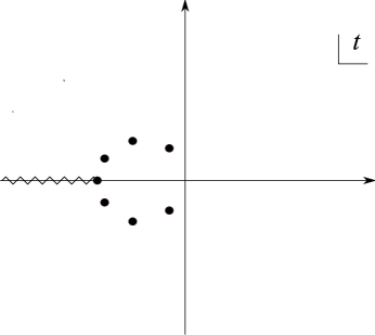
Figure 4: Analytic structure of the $t$ integrand of ${\cal F}^{\text{scalar}}(u;z)$ in the near-singularity region of Schwarzschild spacetime. The branch point lies at the position of the singularity and the other points are double poles.

For scalar QED, the refractive index is given by (133) with the other polarization obtained by swapping the powers $\tfrac{3}{2}\leftrightarrow\tfrac{1}{2}$. Notice that the affine parameter $u$ is negative, with the singularity at $u=0$. In this case, the integrand has a branch point at $t=-|u|$, i.e. when $u^{\prime}$ lies at the singularity, and double poles at

$$t=|u|\big{(}e^{2\pi ip/7}-1\big{)}\ ,\qquad p=1,2,\ldots,6\ .$$ (176)

as shown in Fig.4.

  

Figure 5: $n(\omega)-1$ for the near singularity region of the Schwarzschild black hole plotted as a function of $\log\omega$: continuous (real part, polarization $i=1$); big dashes (imaginary part, $i=1$); small dashes (real part, polarization $i=2$) and dots (imaginary part, $i=2$), for scalar QED (left) and QED (right).

The refractive index in the near singularity limit can be evaluated numerically and the results are shown in Fig.5. As expected for a Ricci flat spacetime, the signs of the corrections are the same for scalar and spinor QED, with both showing birefringence. In this example, however, unlike the case of the Ricci flat symmetric plane wave, the sign of $\operatorname{Im}n(\omega)$ differs for the different polarization states.

7.3 Kerr black hole

The case of the Kerr spacetime describing a rotating black hole can be analyzed in the same way and provides a very nice illustration of the simplicity of the Newman-Penrose tetrad approach. The Kerr metric is:

$$ds^{2}~{}~{}=~{}~{}-\rho^{2}{\Delta\over\Sigma^{2}}dt^{2}~{}+~{}\rho^{2}{1\over\Delta}dr^{2}~{}+~{}\rho^{2}d\theta^{2}~{}+~{}{1\over\rho^{2}}\Sigma^{2}\sin^{2}\theta\bigl{(}d\phi-\omega dt\bigr{)}^{2}\ ,$$ (177)

where $\Delta=r^{2}-2Mr+a^{2}$,  $\Sigma^{2}=(r^{2}+a^{2})^{2}-a^{2}\sin^{2}\theta\Delta$,  $\rho^{2}=r^{2}+a^{2}\cos^{2}\theta$ and $\omega=2Mra/\Sigma^{2}$. The metric is specified by two parameters, $M$ and $a$, where $M$ is the mass and $Ma$ the angular momentum (about the rotation axis $\theta=0$) as measured from infinity. Note that the time component simplifies, $g_{tt}=(1-2Mr/\rho^{2})$.

The condition $\Delta(r)=0$, for which there is a coordinate singularity similar to that in the Schwarzschild metric, has two real solutions, $r=r_{\pm}=M\pm\sqrt{M^{2}-a^{2}}$ (assuming $a<M$). The larger, $r=r_{+}$, is the event horizon. The region $r<r_{-}$ contains a ring singularity. However, for the Kerr metric, this does not coincide with the condition $g_{tt}=0$, which defines the boundary of the region, the ergosphere, where an asymptotically timelike Killing vector becomes spacelike. Within the ergosphere, even null curves are pulled round in the direction of the rotation. Its outer limit $r_{E}(\theta)=M+\sqrt{M^{2}-a^{2}\cos^{2}\theta}$, known as the stationary limit surface, coincides with the event horizon at the poles and is equal to the Schwarzschild radius $2M$ at the equator.

The null geodesics in the Kerr metric have been extensively studied (see ref.[12] for a comprehensive discussion, and [25] for a first analysis of photon propagation in QED). Although the equatorial orbits are of special interest and simplicity, our formalism allows us to consider immediately the general case of non-planar orbits. In this case, analogous to (150), we have $\hat{k}^{\mu}=E^{-1}(\dot{t},\dot{r},\dot{\theta},\dot{\phi})$ where

$$\begin{split}\dot{t}~{}&=~{}{E\over\Delta}\Bigl{(}r^{2}+a^{2}+{2Mra\over\rho^{2}}(a\sin^{2}\theta-b)\Bigr{)}\\ \dot{r}~{}&=~{}{E\over\rho^{2}}\Bigl{(}r^{4}+(a^{2}-b^{2}-q)r^{2}+2Mr\bigl{(}(a-b)^{2}+q\bigr{)}-a^{2}q\Bigr{)}^{1\over 2}\\ \dot{\theta}~{}&=~{}{E\over\rho^{2}}\Bigl{(}q+(a^{2}\sin^{2}\theta-b^{2})\cot^{2}\theta\Bigr{)}^{1\over 2}\\ \dot{\phi}~{}&=~{}{E\over\Delta\sin^{2}\theta}\Bigl{(}b+{2Mr\over\rho^{2}}(a\sin^{2}\theta-b)\Bigr{)}\ .\end{split}$$ (178)

The orbits are characterized by the energy $E$ and two impact parameters, the familiar $b=L_{z}/E$ and $q$, its analogue in the $\theta$-plane [12]. Both are conserved quantities.

Like Schwarzschild, the Kerr spacetime is Petrov type D and the only non-vanishing component of the Weyl tensor is $\Psi_{2}=C_{\ell mn\bar{m}}$ referred to the null basis

$$\begin{split}\ell^{\mu}~{}&=~{}{1\over\Delta}\bigl{(}r^{2}+a^{2},\Delta,0,a\bigr{)}\\ n^{\mu}~{}&=~{}{1\over 2\rho^{2}}\bigl{(}r^{2}+a^{2},-\Delta,0,a\bigr{)}\\ m^{\mu}~{}&=~{}{1\over\sqrt{2}\tilde{\rho}}\bigl{(}ia\sin\theta,0,1,{i\over\sin\theta}\bigr{)}\ ,\end{split}$$ (179)

where $\tilde{\rho}=r+ia\cos\theta$. In this basis, $\Psi_{2}=-{M/({\tilde{\rho}}^{*})^{3}}$.

At this point, we can simply invoke the general discussion of type D spacetimes in section 7.1 to write down the Penrose limit. The Kerr spacetime is Ricci flat, so from (148) we see that the eigenvalues of the plane wave profile function $h_{ij}$ corresponding to the null geodesic with tangent vector $\hat{k}^{\mu}$ are simply

$$h_{ij}~{}=~{}\delta_{ij}(-1)^{i}|\Psi_{2}|~{}\hat{k}\cdot\ell~{}\hat{k}\cdot n\ ,$$ (180)

with $|\Psi_{2}|=M/\rho^{3}$. A straightforward algebraic exercise now shows that

$$\hat{k}\cdot\ell~{}\hat{k}\cdot n~{}=~{}{1\over 2\rho^{2}}\bigl{(}(a-b)^{2}+q\bigr{)}\ ,$$ (181)

consistent with the general theorem that

$$|K_{s}|^{2}~{}=~{}4|\Psi_{2}|^{-{2\over 3}}~{}\hat{k}\cdot\ell~{}\hat{k}\cdot n~{}=~{}2M^{-{2\over 3}}\bigl{(}(a-b)^{2}+q\bigr{)}$$ (182)

is conserved along the geodesic. For the general Kerr orbit, we therefore have

$$h_{11}~{}=~{}-{3M\over\rho^{5}}\bigl{(}(a-b)^{2}+q\bigr{)}\ ,\qquad h_{22}~{}=~{}{3M\over\rho^{5}}\bigl{(}(a-b)^{2}+q\bigr{)}$$ (183)

This is a remarkable simplification and illustrates very clearly the dependence of the Penrose limit on both the spacetime curvature and the characteristics of the chosen null geodesic.

Eq.(183) is a straightforward generalization of the Schwarzschild result (159) and similar consequences follow here. Clearly, the Penrose limit is flat for a principal null geodesic, i.e. $\hat{k}^{\mu}=\ell^{\mu}$. Once again, there is an unstable closed orbit for a constant value $r_{c}$ of the radial coordinate. Imposing $\ddot{r}=0$, and specializing for simplicity to equatorial orbits, determines the relation $r_{c}=3M(b_{c}-a)/(b_{c}+a)$, though here the expression for the critical radius is more complicated, involving the solution of a cubic equation, and we have $r_{c}=2M\Bigl{[}1+\cos\Bigl{(}{2\over 3}\cos^{-1}\bigl{(}\pm{a\over M}\bigr{)}\Bigr{)}\Bigr{]}$ for the retrograde and direct orbits respectively [12]. Evaluating $h_{ij}$ for this orbit, we find the non-vanishing elements

$$h_{11}~{}=~{}-{3\over r_{c}^{2}}~{}=~{}-{1\over 3M^{2}}\Bigl{(}{b_{c}+a\over b_{c}-a}\Bigr{)}^{2}\ ,\qquad h_{22}~{}=~{}{3\over r_{c}^{2}}~{}=~{}{1\over 3M^{2}}\Bigl{(}{b_{c}+a\over b_{c}-a}\Bigr{)}^{2}$$ (184)

Since this is a constant, we confirm that, just as in the Schwarzschild case, the Penrose limit for the critical orbit in Kerr spacetime is a Ricci flat symmetric plane wave.

The near-singularity limit follows straightforwardly. Restricting to equatorial orbits, we determine the small $r$ behaviour of the radial geodesic equation from (178) as

$${\dot{r}}^{2}~{}=~{}{2M(a-b)^{2}\over r^{3}}+{\cal O}\Bigl{(}{1\over r^{2}}\Bigr{)}\ ,$$ (185)

and integrating, we find $r^{5}={25\over 2}M(b-a)^{2}u^{2}$ and therefore the Penrose limit profile function is a homogeneous plane wave identical to the Schwarzschild result (167). This reflects the equivalent power-law nature of the singularities for Schwarzschild and Kerr black holes. This result implies that the singularity behaviour of the refractive index is the same as for the Schwarzschild solution.

7.4 Reissner-Nordstrom black hole

It is very simple to generalize the calculation of the Penrose Limit for the Schwarzschild black hole to the Reissner-Nordstrom black hole. Here we shall simply state the result that

$$h_{11}=-\frac{3Mb^{2}}{r^{5}}+\frac{4b^{2}Q^{2}}{r^{6}}\ ,\qquad h_{22}=\frac{3Mb^{2}}{r^{5}}-\frac{2b^{2}Q^{2}}{r^{6}}\ .$$ (186)

Notice that the hole is not Ricci flat so that

$$R_{uu}=h_{11}+h_{22}=\frac{2b^{2}Q^{2}}{r^{6}}\ .$$ (187)

This result is not as it stands useful for the calculation of the refractive index because in this case there is background electro-magnetic field that would have to be taken into account in addition to the curvature of spacetime [26].

8 Cosmological spacetimes

We now consider a cosmological spacetime with an initial singularity, the Friedmann-Robertson-Walker universe. This example is of more than just conceptual interest since modifications to the speed of light in the very early universe are potentially important in the context of the horizon problem, one of the original motivations for inflation.

The metric for a FRW spacetime has the form

$$ds^{2}~{}=~{}-dt^{2}+a(t)^{2}\Big{[}dr^{2}+f_{\kappa}(r)d\Omega^{2}\Big{]}$$ (188)

where $f_{\kappa}(r)=r$, $\sin r$ and $\sinh r$ for $\kappa=0$, $+1$ and $-1$ respectively, representing a flat, closed or open universe, and $d\Omega^{2}$ is the usual metric for the two-sphere. With no loss of generality, we consider geodesics with zero angular momentum on this transverse space. These null geodesics are well known. We have

$$\dot{t}=\frac{1}{a}\ ,\qquad\dot{r}=\frac{1}{a^{2}}\ ,$$ (189)

Note that we use the notation $\dot{t}\equiv{dt\over du}$ for $u$-derivatives; in what follows we denote $t$-derivatives by $a^{\prime}(t)\equiv{da\over dt}$, etc. Here, $u$ is as usual the affine parameter along the null geodesic $\gamma$. We therefore find $\hat{k}^{\mu}=\bigl{(}a^{-1},a^{-2},0,0\bigr{)}$ in a $(t,r,\theta,\phi)$ coordinate basis.

The first step in finding the Penrose limit by the conventional method [13] described earlier is to identify a parallel transported frame $E_{A}$ along $\gamma$. Here, we have:

$$\begin{split}E_{u}{}^{\mu}~{}\equiv~{}\hat{k}^{\mu}~{}&=~{}\bigl{(}a^{-1},a^{-2},0,0\bigr{)}~{}~{}~{}~{}~{}~{}~{}~{}~{}~{}~{}~{}~{}~{}E_{v}{}^{\mu}~{}=~{}-{1\over 2}\bigl{(}-a,1,0,0\bigr{)}\\ E_{1}{}^{\mu}~{}&=~{}(af_{\kappa})^{-1}\bigl{(}0,0,1,0\bigr{)}~{}~{}~{}~{}~{}~{}~{}~{}~{}~{}E_{2}{}^{\mu}~{}=~{}(af_{\kappa})^{-1}\bigl{(}0,0,0,1/\sin\theta\bigr{)}\end{split}$$ (190)

The matrix $\Omega_{ij}=E_{i}{}^{\mu}E_{j}{}^{\nu}\nabla_{\mu}\hat{k}_{\nu}$  $(i,j=1,2)$  follows straightforwardly and we find after a short calculation that

$$\Omega_{ij}~{}=~{}\delta_{ij}{d\over du}\log(af_{\kappa})\ ,$$ (191)

with $a\equiv a(t(u))$, $f_{\kappa}\equiv f_{\kappa}(r(u))$ along $\gamma$. The profile function for the Penrose plane wave is then

$$h_{ij}~{}=~{}-\delta_{ij}(af_{\kappa})^{-1}{d^{2}\over du^{2}}(af_{\kappa})\ .$$ (192)

This confirms $h_{11}=h_{22}$, as expected since the Penrose limit inherits the conformally flat property of the original FRW metric. Then, since the metric function $f_{\kappa}(r)$ satisfies ${\partial^{2}\over\partial r^{2}}f_{\kappa}+\kappa f_{\kappa}=0$ for all $\kappa$, we readily find [13]

$$h_{ij}~{}=~{}-\delta_{ij}\Bigl{(}{\ddot{a}\over a}-{\kappa\over a^{4}}\Bigr{)}\ .$$ (193)

Finally, to make contact with conventional FRW dynamics, we can re-express this in terms of $t$-derivatives, giving

$$\begin{split}h_{ij}~{}&=~{}-\delta_{ij}{1\over a^{2}}\Bigl{(}{a^{\prime\prime}\over a}-{\kappa+a^{\prime 2}\over a^{2}}\Bigr{)}\\ &=~{}\delta_{ij}{4\pi G\over a^{2}}\rho(1+w)\ ,\end{split}$$ (194)

using the standard Friedmann and acceleration equations,

$$\begin{split}{a^{\prime 2}\over a^{2}}+{\kappa\over a^{2}}~{}&=~{}{8\pi G\over 3}\rho\\ {a^{\prime\prime}\over a}~{}&=~{}-{4\pi G\over 3}(\rho+3p)\end{split}$$ (195)

and the equation of state $p=w\rho$.

The Newman-Penrose null tetrad derivation of the Penrose limit is especially quick in this example. Recall from the discussion in the preceding section that the profile function is given by (142), where here we can identify the NP basis vectors $L,N,M,\bar{M}$ with the $E_{A}{}$ of (190). Since the FRW spacetime is conformally flat, we immediately have

$$h_{ij}~{}=~{}{1\over 2}R_{\mu\nu}E_{u}{}^{\mu}E_{u}{}^{\nu}\delta_{ij}~{}\equiv~{}{1\over 2}R_{uu}\delta_{ij}\ .$$ (196)

To check this with the previous result (194), recall that the Ricci tensor is given by $R_{\mu\nu}=8\pi G(T_{\mu\nu}-{1\over 2}T^{\lambda}{}_{\lambda}g_{\mu\nu})$ where the FRW energy-momentum tensor is $T_{\mu\nu}=(\rho+p)t_{\mu}t_{\nu}+pg_{\mu\nu}$ with $t^{\mu}$ a unit vector in the $t$-direction. It follows immediately that

$$\begin{split}h_{ij}~{}&=~{}{1\over 2}R_{\mu\nu}E_{u}{}^{\mu}E_{u}{}^{\nu}\delta_{ij}\\ &=~{}8\pi G(\rho+p)(E_{u}\cdot t)^{2}\\ &=~{}\delta_{ij}{4\pi G\over a^{2}}(\rho+p)\ ,\end{split}$$ (197)

since the terms proportional to $g_{\mu\nu}$ do not contribute as $E_{u}{}^{\mu}$ is null.

To take this further, we now use the standard conservation equation

$${d\over da}\bigl{(}\rho a^{3}\bigr{)}~{}=~{}-3w\rho a^{2}\ ,$$ (198)

which follows from $\nabla_{\mu}T^{\mu\nu}=0$, to deduce as usual $\rho\sim a^{-3(1+w)}$. It is convenient here to introduce the parameter $\gamma={2\over 3(1+w)}$. The three standard equations of state considered in FRW cosmology are $w=0~{}(\gamma=2/3)$ for non-relativistic matter, $w=1/3~{}(\gamma=1/2)$ for radiation, and $w=-1~{}(\gamma\rightarrow\infty)$ for a cosmological constant. The latter implies a flat Penrose limit, as is evident from (194), since a vacuum spacetime with a cosmological constant, i.e. de Sitter space, is maximally symmetric. Combining (198) with the Friedmann equations, and introducing the constant $C_{\gamma}{8\pi G\over 3}\rho a^{2\over\gamma}$, we now have

$$\begin{split}\kappa+a^{\prime 2}~{}&=~{}C_{\gamma}a^{2(1-{1\over\gamma})}\\ a^{\prime\prime}~{}&=~{}C_{\gamma}\bigl{(}1-\tfrac{1}{\gamma}\bigr{)}a^{1-{2\over\gamma}}\end{split}$$ (199)

showing clearly that $\gamma<1~{}(w<-1/3)$ is the threshold for an accelerating universe. We therefore find from (194) that the Penrose limit profile function is

$$h_{ij}~{}=~{}\delta_{ij}C_{\gamma}\gamma^{-1}a^{-2(1+{1\over\gamma})}\ ,$$ (200)

where the dependence of $a(u)$ on $u$ follows from (199) as

$$u~{}=~{}\int da{a\over\sqrt{C_{\gamma}a^{2(1-{1\over\gamma})}-\kappa}}\ .$$ (201)

It is now simplest to consider the various possible cases separately.

(i)  Spatially flat universe, $\kappa=0$, for any $\gamma$:

In this case, the integral in (201) is trivial and the dependence of $a(u)$ on $u$ is given implicitly by $u=C_{\gamma}^{-1/2}{\gamma\over\gamma+1}a^{1+\gamma^{-1}}$. The profile function (200) follows immediately:

$$h_{ij}~{}=~{}{\gamma\over(\gamma+1)^{2}}{1\over u^{2}}\delta_{ij}\ .$$ (202)

Perhaps unsurprisingly given our experience with black hole spacetimes with singularities in the previous section, we find here that the Penrose limit of a flat FRW spacetime is a conformally flat singular homogeneous plane wave with coefficient $c={\gamma\over(\gamma+1)^{2}}$.

(ii)  $\gamma=1$, for any $\kappa$:

As already noted, an equation of state with $\gamma=1~{}(w=-{1\over 3})$ is on the boundary between a decelerating ($0<\gamma<1$) and accelerating ($\gamma>1$) universe. From the Friedmann equation, we see this requires $C_{1}-\kappa>0$, which only becomes a constraint on the energy density for a closed universe, $\kappa=1$. In this case, we find $u={1\over 2}{1\over\sqrt{C_{1}-\kappa}}a^{2}$, and the profile function can be expressed as

$$h_{ij}~{}=~{}{1\over 4}\Bigl{(}1+{\kappa\over C_{1}-\kappa}\Bigr{)}{1\over u^{2}}\delta_{ij}\ .$$ (203)

Again we find a singular homogeneous plane wave, though with a $\kappa$-dependent modification of the coefficient in (202). The case $\kappa=1$ is interesting in that in this case $\alpha_{i}^{2}=(1-C_{1})^{-1}<0$ and so $\alpha_{i}$ is imaginary and, following the discussion in Section 6.2, there are an infinite sequence of conjugate points.

In these special cases, the characteristic $1/u^{2}$ behaviour of $h_{ij}$ holds exactly for all $u$, i.e. along the whole geodesic. The following results, in contrast, describe only the leading behaviour in the near-singularity limit.

(iii)  Decelerating universe, $0<\gamma<1$, for all $\kappa$:

Here, the first term in the denominator of (201) dominates for small $a$, and the dependence of $a(u)$ on $u$ is exactly as in case(i). So again we find, for all $\kappa$,

$$h_{ij}~{}=~{}{\gamma\over(\gamma+1)^{2}}{1\over u^{2}}\delta_{ij}\ ,$$ (204)

in the near-singularity limit. Notice that for the case of a matter dominated universe, $\gamma=\tfrac{2}{3}~{}(w=0)$, the coefficient in (204) is $\tfrac{6}{25}$, precisely the same as for the near-singularity limit of Schwarzschild, or Kerr, spacetime [13].

(iv)  Accelerating universe, $\gamma>1$:

For an accelerating, $\gamma>1$, universe, we have already found the exact solution (202) for $\kappa=0$. For $\kappa=1$, the Friedmann equation does not have a solution if $a$ becomes too small – the parameters $\kappa=1,\gamma>1$ do not correspond to a spacetime with an initial singularity. This leaves the open universe $\kappa=-1$. This time, for sufficiently small $a$, the second term in the denominator of (201) dominates and we find $u\simeq\tfrac{1}{2}a^{2}$, leading to

$$h_{ij}~{}=~{}\delta_{ij}2^{-(1+{1\over\gamma})}\gamma^{-1}C_{\gamma}{1\over u^{1+{1\over\gamma}}}\ .$$ (205)

The singular behaviour of $h_{ij}$ is softer than $1/u^{2}$ in this case; this can be interpreted as due to a cancellation of the leading $1/u^{2}$ singular behaviour from the two terms in (193) when $u={1\over 2}a^{2}$.

In order to consider the refractive index in these cosmological examples, the following conceptual issue arises. Notice that the expression for the index in (85) and (86), depends on the past history of the geodesic. The intuitive understanding is that a definition of the refractive index involves waves coming in from past null infinity. In an FRW universe, the singularity cuts off this past history and the refractive index cannot, as such, be defined in this way. However, another way to think about the vacuum polarization is in terms of an initial value problem: rather than have the waves come in from past null infinity, one defines a wave at some initial time. In this case one should think in terms of the retarded Green function rather than the refractive index. This quantity was considered in [2]. Effectively defining an initial value problem provides an the upper limit for the $t$ integral in (86) of the form $u_{0}$, where the initial value surface is at $u=u_{0}$:

$$\boldsymbol{\cal F}(u;z)=\int_{0}^{u_{0}-i\epsilon}\frac{dt}{t^{2}}\,ie^{-izt}\left[\boldsymbol{\Delta}\big{(}u,u-t\big{)}\sqrt{{\rm det}\boldsymbol{\Delta}\big{(}u,u-t\big{)}}-\boldsymbol{1}\right]\ ,$$ (206)

The resulting quantity $\boldsymbol{n}(u;\omega)$ then plays the rôle of an effective refractive index for waves that begin on the initial value surface which, therefore, depends implicitly on the choice of the initial value surface.

The presence of the cut-off on the $t$ integral changes the low frequency behaviour of the refractive index from the expressions in (19) and (20) to

$$n_{ij}^{\text{scalar}}(u,u_{0};\omega)=\delta_{ij}-\frac{\alpha}{360\pi m^{2}}\big{(}R_{uu}(u)\delta_{ij}+2R_{uiuj}(u)\big{)}F\Big{(}\frac{\omega}{m^{2}(u-u_{0})}\Big{)}+\cdots\ ,$$ (207)

while for spinor QED,

$$n_{ij}^{\text{spinor}}(u,u_{0};\omega)=\delta_{ij}-\frac{\alpha}{180\pi m^{2}}\big{(}13R_{uu}(u)\delta_{ij}-4R_{uiuj}(u)\big{)}F\Big{(}\frac{\omega}{m^{2}(u-u_{0})}\Big{)}+\cdots\ ,$$ (208)

where

$$F(x)=1-6\int_{0}^{1}d\xi\,\xi(1-\xi)e^{-i/(2\xi(1-\xi)x)}\ .$$ (209)

The effect is that the low-frequency behaviour oscillates as a function of $\omega$.

As an example of the kind of behaviour one encounters with this definition of the refractive index, consider the Milne universe [27] which has spatially flat sections $\kappa=0$ and metric

$$ds^{2}=-dt^{2}+a^{2}t^{2}(dx^{2}+dy^{2}+dz^{2})\ .$$ (210)

A congruence of null geodesics is simply obtained by taking $y$ and $z$ constant along with $\dot{t}=at\dot{x}$, which is solved by taking $x=(2a)^{-1}\log u-x_{0}$, for constant $x_{0}$. The variables $(t,x_{0},y,z)$ form a set of Rosen coordinates for the congruence. Writing the metric in terms of these coordinates we have

$$ds^{2}=-2at\,dt\,dx_{0}+a^{2}t^{2}(dx_{0}^{2}+dy^{2}+dz^{2})\ .$$ (211)

In order to take the Penrose limit, we choose an affine parameter $u=at^{2}/2$ and identify $x_{0}=V$, $Y^{1}=y$ and $Y^{2}=z$. Then the Penrose is easily taken giving, in both Rosen and Brinkmann coordinates,

$$\begin{split}d\hat{s}^{2}&=-2du\,dV+2au\,\big{(}dY^{1}\,dY^{1}+dY^{2}\,dY^{2}\big{)}\\ &=-2du\,dv-\frac{1}{4u^{2}}\big{(}(y^{1})^{2}+(y^{2})^{2}\big{)}du^{2}+dy^{i}\,dy^{i}\ .\end{split}$$ (212)

This is precisely a singular homogeneous plane wave of the type discussed in Section 6.2 with $\alpha_{i}=0$ and the VVM matrix may be extracted from (131) by taking the limit $\alpha_{i}\to 0$:

$$\Delta_{ij}(u,u^{\prime})=\delta_{ij}\frac{u-u^{\prime}}{\sqrt{uu^{\prime}}\log(u/u^{\prime})}\ .$$ (213)

Numerical evaluations of the refractive index are shown in figure 6 for scalar and spinor QED. In this case the spacetime is conformally flat and so there is no bi-refringence. At low frequency we see the characteristic oscillations that match (207) and (208).

(a)          (b)

Figure 6: $\text{Re}\,n-1$ (continuous) and $\text{Im}\,n$ (dashed) plotted as a function of $\log\omega$ in suitable units for the Milne universe for (a) scalar QED and (b) spinor QED.

9 Gravitational Waves

Finally, we consider another major class of spacetimes – gravitational waves. Two examples are studied in detail, viz. weak gravitational waves and gravitational shockwaves, the latter being of particular interest because of the use of the Aichelburg-Sexl metric [28] in investigations of Planck energy scattering in quantum gravity.

9.1 Weak gravitational waves

The spacetime metric for a weak gravitational wave has the following form in Rosen coordinates:

$$ds^{2}~{}=~{}-2du\,dV+(1+\epsilon\cos\nu u)dY^{1}\,dY^{1}+\big{(}1-\epsilon\cos\nu u\big{)}dY^{2}\,dY^{2}\ .$$ (214)

Here, and in the following, $\epsilon$ is small and we work to linear order. The transformation to Brinkmann coordinates is made using the zweibein

$$E_{a}{}^{j}(u)=\delta_{a}^{i}\big{(}1-(-1)^{j}\frac{\epsilon}{2}\cos\nu u\big{)}\ ,$$ (215)

giving

$$ds^{2}~{}=~{}-2du\,dv-\frac{\epsilon\nu^{2}}{2}\cos\nu u\big{[}(y^{1})^{2}-(y^{2})^{2}\big{]}\,du^{2}+dy^{j}\,dy^{j}\ .$$ (216)

Since $h_{11}=-h_{22}={1\over 2}\epsilon\nu^{2}\cos\nu u$, this is a Ricci flat spacetime and, as usual, will display gravitational birefringence.

The metric (216) is already in the form of the Penrose limit for a photon travelling in the opposite direction to the gravitational wave along the null geodesic given by (54). Notice that a photon travelling in the same direction as the gravitational wave has a flat Penrose limit and there is no vacuum polarization effect on its refractive index [5, 29].

The Jacobi fields therefore satisfy

$$\frac{d^{2}y^{(\pm)}}{du^{2}}\pm\frac{\epsilon\nu^{2}}{2}\cos\nu u\,y^{(\pm)}=0\ ,$$ (217)

where we have labelled the two polarizations $y^{(+)}\equiv y^{1}$ and $y^{(-)}\equiv y^{2}$. This can easily be solved perturbatively in $\epsilon$, with solution to linear order

$$y^{(\pm)}(u)=c_{1}+uc_{2}\pm\frac{\epsilon}{2}(c_{1}+uc_{2})\cos\nu u\mp\frac{\epsilon c_{2}}{\nu}\sin\nu u\ .$$ (218)

The (diagonal) matrix $\boldsymbol{A}(u,u^{\prime})$ is the solution of the Jacobi equation subject to the now-familiar boundary conditions and we find its components for the tow polarizations to be

$$\begin{split}A_{(\pm)}(u,u^{\prime})~{}=~{}&u-u^{\prime}\\ &\pm\frac{\epsilon(u-u^{\prime})}{2}\big{(}\cos\nu u+\cos\nu u^{\prime}\big{)}\mp\frac{\epsilon}{\nu}\big{(}\sin\nu u-\sin\nu u^{\prime}\big{)}\ .\end{split}$$ (219)

This determines the eigenvalues of the Van-Vleck Morette matrix:

$$\Delta_{(\pm)}(u,u^{\prime})~{}=~{}1\mp\frac{\epsilon}{2}(\cos\nu u+\cos\nu u^{\prime})\pm\frac{\epsilon}{\nu(u-u^{\prime})}(\sin\nu u-\sin\nu u^{\prime})\ .$$ (220)

Notice that this is regular for all $u,u^{\prime}$, reflecting the fact that in this weak field (small $\epsilon$) approximation there are no conjugate points in the null geodesic congruence.

The refractive index for scalar QED is given as usual by (82) where for the 2 polarizations we have

$$\begin{split}{\cal F}^{\text{scalar}}_{(\pm)}(u;z)&=\mp\epsilon\int_{0}^{\infty-i\epsilon}\frac{dt}{t^{2}}\,ie^{-izt}\\ &~{}~{}~{}\times\Big{[}\frac{1}{2}(\cos\nu u+\cos\nu(u-t))-\frac{1}{\nu t}(\sin\nu u-\sin\nu(u-t))\Big{]}\\ &=\pm\epsilon\big{[}f(z)\cos\nu u+g(z)\sin\nu u\big{]}\ ,\end{split}$$ (221)

with

$$\begin{split}f(z)~{}&=~{}\frac{z}{4\nu}\big{[}2\nu(1+\log z)+(z-\nu)\log(z-\nu)-(z+\nu)\log(z+\nu)\big{]}\ ,\\ g(z)~{}&=~{}\frac{i}{4\nu}\big{[}\nu^{2}+2z^{2}\log z+z(\nu-z)\log(z-\nu)-z(z+\nu)\log(z+\nu)\big{]}\ .\end{split}$$ (222)

For spinor QED the only difference relative to scalar QED is an overall multiple of 4:

$${\cal F}^{\text{spinor}}_{(\pm)}(u;z)=4{\cal F}^{\text{scalar}}_{(\pm)}(u;z)\ ,$$ (223)

and so we will continue to discuss the scalar case.

The functions $f(z),~{}g(z)$ have branch points at $0$, $\infty$ and $z=\pm\nu$ and this means that $n_{(\pm)}(u;\omega)$ will have branch points at 0 $\pm\infty$ and $\pm 2m^{2}/\nu$. In particular, the branch points at $\pm 2m^{2}/\nu$ are points of non-analyticity of the refractive index. This non-analyticity manifests itself by the fact that $\text{Im}\,f(z)$ and $\text{Re}\,g(z)$ are zero for $z\in{\bf R}>\nu$, while for $z\in{\bf R}<\nu$,

$$\text{Im}\,f(z)=\text{Re}\,g(z)=\frac{\pi z(\nu-z)}{4\nu}\ .$$ (224)

The low frequency expansion of the refractive index follows immediately from (221), (222) and we find:

$$\begin{split}n^{(\pm)}(u;\omega)~{}=~{}1~{}&\pm~{}\frac{\alpha\epsilon\nu^{2}}{m^{2}\pi}\Big{[}\frac{1}{360}+\frac{1}{6300}\left(\frac{\omega\nu}{m^{2}}\right)^{2}++\cdots\Big{]}\cos\nu u\\ &\mp~{}i\frac{\alpha\epsilon\nu^{2}}{m^{2}\pi}\Big{[}\frac{1}{840}\left(\frac{\omega\nu}{m^{2}}\right)+\frac{1}{10395}\left(\frac{\omega\nu}{m^{2}}\right)^{3}+\cdots\Big{]}\sin\nu u\ ,\end{split}$$ (225)

while at high frequencies,

$$n^{(\pm)}(u;\omega)=1\pm i\frac{\alpha\epsilon\nu}{6\pi\omega}\sin\nu u+\cdots$$ (226)

Notice that the low frequency expansion is not sensitive to the non-perturbative contribution (224). The leading terms for both real and imaginary parts can however be read off from the effective Lagrangian described in section 2.

(a)          (b)

Figure 7: $\text{Re}\,n-1$ and $\text{Im}\,n$ for the 2 polarizations (a) and (b) for $u=0.2$, $m=\nu=1$ plotted as a function of $\log\nu\omega/m^{2}$ in units of $\epsilon\alpha$ for both polarizations. The point of non-analyticity at $\omega=2m^{2}/\nu$ is quite clear. (Note that the fact that the polarizations do not quite give mirror images is an artifact of the numerical approximation.

The full form of the frequency dependence of the real and imaginary parts of the refractive index is plotted numerically in Fig. 7, evaluated at a fixed point on the photon trajectory, for both scalar and spinor QED. For the first polarization, has a $\operatorname{Re}n(\omega)$ which qualitatively looks similar to a conventional dielectric with a single characteristic frequency $\omega\sim m^{2}/\nu$, together with an imaginary part $\operatorname{Im}n(\omega)$ which is negative in the perturbative small $\omega$ regime before being dominated by the positive non-perturbative contribution (224) above the branch point at $\omega=2m^{2}/\nu$. Since this is a Ricci flat spacetime, the second polarization has the opposite sign, being superluminal at low frequencies and with $\operatorname{Im}n(\omega)<0$ above the branch point, normally an indication of amplification rather than dispersive scattering. The roles of the two polarizations of course change along the photon trajectory through the background gravitational wave.

9.2 Gravitational shockwaves

A gravitational shockwave is described by the Aichelburg-Sexl metric [28]

$$ds^{2}=-2du\,dv+f(r)\delta(u)\,du^{2}+dx^{2}+dy^{2}\ ,$$ (227)

where $x=r\cos\phi$ and $y=r\sin\phi$. This describes an axis symmetric, plane-fronted wave moving at the speed of light, with a profile function $f(r)$ in the transverse direction determined by the nature of the source: a matter source $T_{uu}=\rho(r)\delta(u)$ corresponds to a profile function satisfying $\Delta f(r)=-16\pi\rho(r)$, where $\Delta$ is the 2-dim Laplacian. We consider two sources of special interest: a particle with $\rho(r)=\mu\delta(\underline{x})$, which gives a profile function $f(r)=-4\mu\log r^{2}$, and a homogeneous beam $\rho(r)=\mu$, for which $f(r)=-4\pi\mu r^{2}$.

The AS metric has many applications in general relativity and more recently in quantum gravity and string theory, where it has been widely used in investigations of Planck energy scattering (see refs.[30, 31, 32] for a selection of papers). Recently, string scattering in a classical AS metric has been studied [33] as a model of Planck scattering, and it would be interesting to compare these results, characterized by the string scale, with the equivalent QFT scattering, where the scale is set by the Compton wavelength of the particle in the vacuum polarization loop. For now, we focus on the effect of a shockwave collision on the refractive index in QED.

The null geodesics describing a photon travelling in the opposite direction to the gravitational shockwave are well-known; those corresponding to a homogeneous beam were first discussed by Ferrari, Pendenza and Veneziano in ref.[34] (see also [35]). With $u$ as the affine parameter, they satisfy

$$\begin{split}r&=R+\tfrac{1}{2}f^{\prime}(R)u\theta(u)\ ,\\ v&=V+\tfrac{1}{2}f(R)\theta(u)+\tfrac{1}{8}f^{\prime}(R)^{2}u\theta(u)\ ,\\ \phi&=\Phi\ ,\end{split}$$ (228)

where $(V,R,\Phi)$ are constants which label a congruence of null geodesics. Consequently, these variables are a natural set of Rosen coordinates. It is now straightforward to change variables from $(u,v,r,\phi)$ to $(u,V,R,\Phi)$:

$$\begin{split}dr&=dR+\tfrac{1}{2}f^{\prime\prime}(R)u\theta(u)dR+\tfrac{1}{2}f^{\prime}(R)\theta(u)du,\\ dv&=dV+\tfrac{1}{2}f^{\prime}(R)\theta(u)dR+\tfrac{1}{2}f(R)\delta(u)du\\ &\qquad+\tfrac{1}{4}f^{\prime}(R)f^{\prime\prime}(R)u\theta(u)dR+\tfrac{1}{8}f^{\prime}(R)^{2}\theta(u)du\ ,\\ d\phi&=d\Phi\ ,\end{split}$$ (229)

where we used the consistent replacement $u\delta(u)\to 0$. The metric in Rosen coordinates is therefore

$$ds^{2}=-2du\,dV+\Big{(}1+\tfrac{1}{2}f^{\prime\prime}(R)u\theta(u)\Big{)}^{2}dR^{2}+\Big{(}R+\tfrac{1}{2}f^{\prime}(R)u\theta(u)\Big{)}^{2}d\Phi^{2}\ .$$ (230)

We can now calculate the Penrose limit around a geodesic with $R=R_{0}$ by defining shifted Rosen coordinates

$$Y^{1}=R-R_{0},\qquad Y^{2}=R_{0}\Phi\ ,$$ (231)

The metric is now in standard form and it is trivial to implement the Penrose limit; we find

$$d\hat{s}^{2}=-2du\,dV+\Big{(}1+\tfrac{1}{2}f^{\prime\prime}(R_{0})u\theta(u)\Big{)}^{2}(dY^{1})^{2}+\Big{(}1+\tfrac{1}{2}R_{0}^{-1}f^{\prime}(R_{0})u\theta(u)\Big{)}^{2}(dY^{2})^{2}\ .$$ (232)

The zweibein $E^{i}{}_{a}(u)$ can be read off directly (see (51)), and has non-vanishing components

$$E^{1}{}_{1}(u)=1+\tfrac{1}{2}f^{\prime\prime}(R_{0})u\theta(u)\ ,\qquad E^{2}{}_{2}(u)=1+\tfrac{1}{2}R_{0}^{-1}f^{\prime}(R_{0})u\theta(u)\ .$$ (233)

We therefore find the Penrose limit in Brinkmann coordinates, with a diagonal profile function $h_{ij}$ given by (55) as

$$h_{11}(u)=-\tfrac{1}{2}f^{\prime\prime}(R_{0})\delta(u)\ ,\qquad h_{22}(u)=-\tfrac{1}{2}R_{0}^{-1}f^{\prime}(R_{0})\delta(u)\ .$$ (234)

For the “particle” AS metric with $f(r)=-4\mu\log r^{2}$ we have

$$h_{ij}(u)=(-1)^{i}\delta_{ij}\frac{4\mu}{R_{0}^{2}}\delta(u)\ ,$$ (235)

which is an example of a Ricci flat plane wave. The related “beam” AS metric with $f(r)=-\mu r^{2}$ gives

$$h_{ij}(u)=\delta_{ij}\mu\delta(u)\ ,$$ (236)

which is a conformally flat shockwave.

The Van Vleck-Morette matrix is found as usual by solving the Jacobi equations subject to the appropriate boundary conditions, with $h_{ij}$ given by (235), (236). Writing the above zweibeins as $E^{i}{}_{a}=\bigl{(}1-\lambda_{i}u\theta(u)\bigr{)}\delta^{i}{}_{a}$,  so that $h_{ij}=\lambda_{i}\delta_{ij}$,  we find, in general, if $u$ and $u^{\prime}$ are on different sides of the shockwave, $uu^{\prime}<0$,

$$\Delta_{ij}(u,u^{\prime})~{}=~{}\frac{|u-u^{\prime}|}{|u-u^{\prime}|+\lambda_{i}uu^{\prime}}\delta_{ij}\ ,$$ (237)

while $\Delta_{ij}(u,u^{\prime})=1$  if $u,u^{\prime}$ are on the same side of the shockwave, $uu^{\prime}>0$. When $uu^{\prime}<0$ for a polarization with $\lambda_{i}>0$, there are conjugate points with $|u|+|u^{\prime}|=\lambda_{i}|uu^{\prime}|$ provided the gravitational field of the shockwave is sufficiently strong, $\lambda_{i}|u|>1$ and $\lambda_{i}|u^{\prime}|>1$. In fact, the relation for conjugate points is

$$\frac{1}{|u|}+\frac{1}{|u^{\prime}|}=\lambda_{i}\ ,$$ (238)

which is the lens formula for a lens of focal length $\lambda_{i}^{-1}$. When the $\lambda_{i}>0$ the lens is converging and a conjugate point exists as long as $u$ and $u^{\prime}$ are large enough, as above. In this case, the refractive index integral will have a branch point on the real $t$ axis. Correspondingly, when $\lambda_{i}<0$ the lens is diverging and no conjugate points exist.

The refractive index is given by the formulae in sections 4 ad 5 and is easily evaluated for both the particle (Ricci-flat) and beam (conformally flat) AS spacetimes with either scalar or spinor QED. For example, consider the conformally flat shockwave and scalar QED. We have, for either polarization,

$$\begin{split}{\cal F}(u;z)~{}&=~{}\theta(u)\int_{u}^{\infty-i\epsilon}\frac{dt}{t^{2}}\,ie^{-izt}\,\left[\Big{(}\frac{t}{t+\lambda u(u-t)}\Big{)}^{2}-1\right]\ ,\\ &=~{}\theta(u)\Big{[}z\Gamma(-1,iuz)-\frac{z}{(1-u\lambda)^{2}}e^{\tfrac{i\lambda u^{2}z}{1-\lambda u}}\Gamma\big{(}-1,\tfrac{iuz}{1-\lambda u}\big{)}\Big{]}\end{split}$$ (239)

where $\Gamma(a,z)=\int_{z}^{\infty}t^{a-1}e^{-t}\,dt$ is the incomplete gamma function. Notice that the lower limit of the integral is at $t=u$, in order that the point $u^{\prime}=u-t<0$ is on the other side of the shockwave. The factor of $\theta(u)$ ensures that the shockwave lies in the past of the point $u$.

In this case, $\lambda$ is negative and the integrand of ${\cal F}(u;z)$ has no poles or branch points on the real $t$ axis. Nevertheless, inspection of the explicit solution in terms of gamma functions makes it clear that ${\cal F}(u;z)$ itself still has branch cuts from $z=0$ to $\infty$. The refractive index $n(\omega)$ evaluated numerically from (239) is shown in Fig. 8.

  

Figure 8: $n-1$ (real part continuous, imaginary part dashed) for $\lambda=1$ and $u=2$ (left) and $u=\tfrac{1}{2}$ (right) plotted as a function of $\log\omega$ for scalar QED.

The small $\omega$ behaviour of the refractive index can be obtained analytically by expanding the integrand of ${\cal F}_{+}(u;z)$ in powers of $t-u$. In all cases,

$$\begin{split}{\cal F}(u;z)~{}&=~{}\theta(u)\int_{u}^{\infty-i\epsilon}dt\,ie^{-izt}\,\Big{[}-\lambda a_{0}(t-u)^{\gamma}/u^{\gamma+1}+{\cal O}(t-u)^{2}\Big{]}\\ &=-i\theta(u)a_{0}e^{-izu}(izu)^{-\gamma-1}\Gamma(1+\gamma)+\cdots\ ,\end{split}$$ (240)

where, depending on the case, $\gamma=0$ or $1$ and $a_{0}$ is some $\lambda u$ dependent constant. The $\xi$ integral is then dominated by a stationary phase with $\xi=\tfrac{1}{2}$ which gives a behaviour

$$n(u;\omega)~{}\underset{\omega\to 0}{=}~{}1+\alpha C(u,m,\lambda)\theta(u)\omega^{\gamma+1/2}e^{-2im^{2}u/\omega}\ ,$$ (241)

where $C(u,m,\lambda)$ is some $\omega$ independent factor. This shows clearly how in this case the non-vanishing imaginary part of the refractive index arises from the oscillating phase factor in the integrand evaluated at the lower limit of the $t$-integral, even though there are no singularities or branch points off the real axis. We can make these formulae even more explicit for the conformally flat scalar QED case. In this case from (239), we get

$$n(u;\omega)~{}\underset{\omega\to 0}{=}~{}1+\alpha\lambda\sqrt{\frac{i\pi\omega^{3}}{2^{11}u^{5}m^{10}}}\theta(u)e^{-2ium^{2}/\omega}\ .$$ (242)

On the other hand, for large $\omega$,

$$n(u;\omega)~{}\underset{\omega\to\infty}{=}~{}1+\frac{i\alpha\lambda}{12(u\lambda-1)\omega}\theta(u)+\log(c\,\omega)\,{\cal O}\Big{(}\frac{1}{\omega^{2}}\Big{)}\ .$$ (243)

Note the oscillations at small $\omega$ as shown in the numerical evaluation in Fig. 8.

It is worth pointing out that in this case we cannot match the low frequency behaviour to the effective action because the curvature is not differentiable. The other thing this computation makes clear is the non-local natural of vacuum polarization: the refractive index is non-trivial even in a region of flat space because the $e^{+}e^{-}$ loop can extend far enough back in time to touch the shockwave.

10 Discussion

The propagation of light, and other quantum fields, is a fundamental and difficult problem for QFT in curved spacetime. In particular, it has raised the question of how the original Drummond and Hathrell discovery of low-frequency superluminal propagation could be consistent with causality. In our previous work, we have resolved this issue by developing techniques which allow an explicit computation of the full frequency dependence of the refractive index and Green functions for (scalar) QED in curved spacetime.

In the present paper, we have further developed the “phenomenology” of the refractive index in a number of important spacetimes, namely black holes, gravitational waves and FRW universes, and extended our analysis to spinor QED. A crucial observation is that, to leading order in $R/m^{2}$, the refractive index depends only on the Penrose limit of the background spacetime around the original null geodesic. This is a very powerful simplification and reveals a number of universal features. For example, propagation in many examples reduces in the Penrose limit to the simple case of homogeneous plane waves, especially the singular homogeneous plane waves which are associated with the near-singularity limits for both black holes and cosmological spacetimes.

A key element in understanding the causal properties of light propagation, and more generally the retarded and advanced Green functions, is the analytic structure of the refractive index. As we have shown, this is in turn controlled by the Van Vleck-Morette matrix which describes the geometry of geodesic deviation. The examples we have studied here display a rich variety of analytic structures, very different from the simple picture in flat spacetime. The Green functions and refractive index therefore display many interesting and physically important features special to curved spacetimes; in particular, conventional dispersion relation theory in QFT, exemplified by the Kramers-Kronig relation, is radically changed. Nevertheless, in all cases we have investigated, the analytic structure still allows the definition of retarded and advanced Green functions with the required causal properties. We can conclude that QED in curved spacetime is indeed a perfectly causal theory despite the unusual and remarkable occurrence of superluminal phase velocities at low frequencies.

Whilst this goal has been achieved and one can finally see explicitly how a low-frequency phase velocity bigger than $c$ is compatible with retarded Green functions that vanish outside the lightcone, a new puzzle arises in that the imaginary part of the refractive index is found in many examples to be negative. This indicates that the optical theorem is violated in curved spacetime. A full explanation of this phenomenon will be presented elsewhere [8].

**********************************

TJH and GMS acknowledge the support of STFC grant ST/G000506/1. RS would like to acknowledge the support of STFC studentship ST/F00706X/1.

References

- [1]
- [2] T. J. Hollowood and G. M. Shore, JHEP 0812 (2008) 091 [arXiv:0806.1019 [hep-th]].
- [3] T. J. Hollowood and G. M. Shore, “The Refractive Index of Curved Spacetime: the Fate of Causality in QED,” Nucl. Phys. B 795 (2008) 138 [arXiv:0707.2303 [hep-th]].
- [4] T. J. Hollowood and G. M. Shore, “Causality and Micro-Causality in Curved Spacetime,” Phys. Lett. B 655 (2007) 67 [arXiv:0707.2302 [hep-th]].
- [5] I. T. Drummond and S. J. Hathrell, Phys. Rev. D 22 (1980) 343.
- [6] G. M. Shore, “Causality and Superluminal Light”, in ‘Time and Matter’, Proceedings of the International Colloquium on the Science of Time, ed. I. Bigi and M. Faessler, World Scientific, Singapore, 2006. [arXiv:gr-qc/0302116].
- [7] G. M. Shore, Nucl. Phys. B 778 (2007) 219 [arXiv:hep-th/0701185].
- [8] T. J. Hollowood and G. M. Shore, to appear.
- [9] R. Penrose, “Any space-time has a plane wave as a limit”, in: Differential geometry and relativity, Reidel and Dordrecht (1976), 271-275.
- [10] G. M. Shore, Contemp. Phys. 44 (2003) 503 [arXiv:gr-qc/0304059].
- [11] M. Walker and R. Penrose, Commun. Math. Phys. 18 (1970) 265.
- [12] S. Chandresekhar, “The Mathematical Theory of Black Holes”, Clarendon, Oxford, 1985.
- [13] M. Blau, “Lecture Notes on Plane waves and Penrose limits”, Based on lectures originally given at the 2004 Saalburg/Wolfersdorf Summer School, http://www.unine.ch/phys/string/Lecturenotes.html
- [14] G. M. Shore, Nucl. Phys. B 646 (2002) 281 [arXiv:gr-qc/0205042].
- [15] G. M. Shore, Nucl. Phys. B 633 (2002) 271 [arXiv:gr-qc/0203034].
- [16] A. O. Barvinsky, Yu. V. Gusev, G. A. Vilkovisky and V. V. Zhytnikov, Print-93-0274 (Manitoba), 1993.
- [17] R. M. Wald, “General Relativity”, Chicago University Press, 1984.
- [18] M. Blau, D. Frank and S. Weiss, Class. Quant. Grav. 23 (2006) 3993 [arXiv:hep-th/0603109].
- [19] H. Kleinert, “Path Integrals”, World Scientific, Singapore, 2004.
- [20] G. M. Shore, Nucl. Phys. B 460 (1996) 379 [arXiv:gr-qc/9504041].
- [21] P. Szekeres and V. Iyer, Phys. Rev. D 68 (1993) 4362.
- [22] M. Célérier and P. Szekeres, Phys. Rev. D 65 (2002) 123516 [arXiv:gr-qc/0203094].
- [23] M. Blau, M. Borunda, M. O’Loughlin and G. Papadopoulos, Class. Quant. Grav. 21 (2004) L43 [arXiv:hep-th/0312029].
- [24] M. Blau, M. Borunda, M. O’Loughlin and G. Papadopoulos, JHEP 0407 (2004) 068 [arXiv:hep-th/0403252].
- [25] R. D. Daniels and G. M. Shore, Phys. Lett. B 367, 75 (1996) [arXiv:gr-qc/9508048].
- [26] R. D. Daniels and G. M. Shore, Nucl. Phys. B 425, 634 (1994) [arXiv:hep-th/9310114];
- [27] N. D. Birrell and P. C. W. Davies, “Quantum fields in curved space”, Cambridge University Press, 1982.
- [28] P. C. Aichelburg and R. U. Sexl, Gen. Rel. Grav. 2 (1971) 303.
- [29] G. M. Shore, Nucl. Phys. B 605 (2001) 455 [arXiv:gr-qc/0012063].
- [30] D. Amati, M. Ciafaloni and G. Veneziano, Phys. Lett. B 197 (1987) 81; Int. J. Mod. Phys. A 3 (1988) 1615; Nucl. Phys. B 347 (1990) 550; JHEP 0802 (2008) 049.
- [31] D. J. Gross and P. F. Mende, Phys. Lett. B 197 (1987) 129; Nucl. Phys. B 303 (1988) 407.
- [32] G. Veneziano, JHEP 0411 (2004) 001 [arXiv:hep-th/0410166].
- [33] S. B. Giddings, D. J. Gross and A. Maharana, Phys. Rev. D 77 (2008) 046001 [arXiv:0705.1816 [hep-th]].
- [34] V. Ferrari, P. Pendenza and G. Veneziano, Gen. Rel. Grav. 20 (1988) 1185.
- [35] G. M. Shore, Int. J. Mod. Phys. A 18 (2003) 4169 [arXiv:gr-qc/0210048].
- [36]