Extra condition is necessary to have a unique cluster wave vectors set in the periodic cluster approximations.

Abstract

We added an extra condition, original lattice symmetry of chosen cluster around cluster central site, to the cluster approximation methods with periodic boundary condition such as dynamical cluster approximation (DCA), effective medium approximation (EMSCA) and nonlocal coherent potential approximation (NLCPA). For each cluster size, this condition leads to a unique cluster wave vectors set in the first Brillouin zone (FBZ) where they preserve full symmetry of first Brillouin zone around ${\bf K=0}$. In this case whole cluster wave vectors are restricted to the FBZ and when number of sites in the cluster is equal to the whole lattice sites, these approximations recover original lattice symmetry in real and k-spaces.

I Introduction

Different single site approximations such as coherent potential approximation (CPA)Soven67 , cluster approximations such as cluster CPA with open boundary condition, dynamical cluster approximation (DCA)Hettler98 ; Jarrell01 ; Jarrell01-2 and effective medium super-cell approximation (EMSCA)Moradian02 ; Moradian04 ; Moradian06 with periodic boundary condition are used to approximate self energy of interacting disordered systems. In the single site approximations the k dependent of self energy is neglected while in the cluster approximations such as DCAHettler98 for interacting and disordered systems, NLCPAMoradian02 for disordered systems and EMSCAMoradian06 in general for interacting disordered systems the cluster wave vector, K, dependent of self energy are considered. The DCA originally constructed in the k-space by dividing the first Brillouin zone (FBZ) in to $N_{c}$ cells. The wave vectors at center of these cells are called cluster wave vectors and denoted by $\{{\bf K}_{1},...,{\bf K}_{N_{c}}\}$. They claimed these cluster wave vectors, ${\bf K}$, are corresponds to a real cluster with periodic boundary conditionHettler98 . But for some clusters there are many possible sets of cluster wave vectors, $\{{\bf K}\}$,Rowlands08 where some of cluster wave vectors are in the higher Brillouin zones. Recently to consider contributions of such different sets of cluster wave vectors, $\{{\bf K}\}$, the origin of FBZ fixed at ${\bf K}=(0,0,0)$ and a phase $\phi$ added to the cluster orthogonality condition,

$$\frac{1}{N_{c}}\sum_{\bf K}e^{i{\bf K}.{\bf r}_{IJ}-i\phi}=\delta_{IJ}.$$ (1)

They claimed, when number of lattice sites $N_{c}\rightarrow\infty$ the phase, $\phi$, goes to zero and this relation converts to the following original lattice orthogonality condition,

$$\frac{1}{N}\sum_{\bf k}e^{i{\bf k}.{\bf r}_{ij}}=\delta_{ij}.$$ (2)

Their uncorrected assumptions and results are due to two factors, first their chosen cluster sizes haven’t original lattice symmetry around cluster central site because this could lead to existence of different set of cluster wave vectors where some of wave vectors are in the higher BZs. Second, the Born von Karman periodic boundary condition, ${\bf k.L}=2\pi n$Ashcroft87 , imply that maximum number of cluster sites, $N_{c}$, should be the whole lattice sites $N$, not $N_{c}\rightarrow\infty$. So in this limit their defined $\phi$ is not going to zero, hence their orthogonality condition Eq.1 is not converting to the original lattice orthogonality condition Eq.2. Since real lattice sites and allowed wave vectors in the FBZ have a one to one correspondence, hence for each cluster with $N_{c}$ sites, it must exist a unique set of $N_{c}$ cluster wave vectors ${\bf K}$ in the FBZ. Therefore we must add an extra condition to the periodicity of clusters with $N_{c}$ sites to have whole cluster wave vectors in the FBZ and just a unique set of super-cell wave vectors ${\bf K}$. Although periodicity condition for such real space clusters are consideredHettler98 ; Jarrell01 ; Jarrell01-2 ; Moradian02 but symmetry of original lattice around central lattice site of clusters are not considered. This is the weakness point of DCA and NLCPA where such symmetry are not considered. By considering both periodicity and lattice symmetry conditions for clusters, size of super-cells limit to those clusters that we can define the Wigner-Seitz cell (WSC) for their central sites and if we translate this WSC by cluster sites vectors set, $\{{\bf r}_{sc}\}$, where defined with respect to the central cluster site, they cover whole cluster with out overlapping. For a 2 dimensional square lattice (2d) this is illustrated in Figure 1. This important condition lead to interesting result where for each cluster there is a unique super-cell wave vectors, $\{{\bf K}\}$, with full FBZ symmetry around ${\bf K}=(0,0,0)$. Here we reformulate the EMSCA in the real space to clarify this problem.

II Model and formalism

We start our investigation by a general tight binding model for a disorder alloy system which is given by,

$$H = -\sum_{ij\sigma\sigma}t_{ij}c^{\dagger}_{i\sigma}c_{j\sigma}$$ (3)

$$+ \sum_{i\sigma}(\varepsilon_{i}-\mu)c^{\dagger}_{i\sigma}c_{i\sigma},$$

where $c^{\dagger}_{i\sigma}$ ($c_{i\sigma}$) is the creation (annihilation) operator of an electron with spin $\sigma$ on lattice site $i$ and $\hat{n}_{i\sigma}=c^{\dagger}_{i\sigma}c_{i\sigma}$ is the number operator. $t^{\sigma\sigma}_{ij}$ are the random hopping integrals between $i$ and $j$ lattice sites with spin $\sigma$ respectively. $\mu$ is the chemical potential and $\varepsilon_{i}$ is the random on-site energy, where takes $0$ with probability $1-c$ for the host sites and $\delta$ with probability $c$ for impurity sites.

The equation of motion for electrons corresponding to the above Hamiltonian, Eq.3, is given by,

$$\sum_{l}\left(\begin{array}[]{c}(E-\varepsilon_{i}+\mu)\delta_{il}-t_{il}\end{array}\right){G}(l,j)=\delta_{ij}$$ (5)

where $G(i,j)$ is the random single particle Green function. Eq.5 could be rewrite as

$$G(E;i,j)=G^{0}(E;i,j)+\sum_{l}G^{0}(E;i,l)\mbox{\boldmath$\varepsilon$}_{l}G(E;l,j).$$ (6)

The Dyson equation corresponding to Eq.5 for the exact averaged Green function, ${\bar{G}}(l,j)$, isziman:79 ,

$${\bar{G}}(E;i,j)=G^{0}(E;i,j)+\sum_{ll^{\prime}}G^{0}(E;i,l)\Sigma(E;l,l^{\prime})G(E;l^{\prime},j)$$ (7)

where the real space self energy matrix, ${\bf\Sigma}$, is defined by,

$$\langle\mbox{\boldmath$\varepsilon$}{\bf G}\rangle={\bf\Sigma}\bar{{\bf G}}$$ (8)

By eliminate clean system Green function $G^{0}$ between Eqs.7 and 8, the exact random Green function ${\bf G}$ could be expand in terms of exact average Green function $\bar{\bf G}$ and exact self energy ${\bf\Sigma}$ as,

$${\bf G}=\bar{\bf G}+\bar{\bf G}(\mbox{\boldmath$\varepsilon$}-{\bf\Sigma}){\bf G}.$$ (9)

Note that although Eqs.6, 7 and 9 are exact but no exact solutions for them. So they should be solved approximately. In the next section by adding original lattice symmetry condition to the chosen super-cell, we reformulate the effective medium super-cell approximation (EMSCA). In this new formalism we show for any super-cell size with periodicity and original lattice symmetry conditions not only there is a unique set of super-cell wave vectors ${\bf K}$ but also all super-cell wave vectors occur in the FBZ with its symmetry.

III Reformulation of the effective medium super-cell approximation

In the EMSCA the real lattice is divided in to the similar super-cells such that each super-cell have whole original lattice symmetry around it’s central site. This means that for each super-cell, if any one sit on it’s central lattice site, exactly see whole lattice symmetryMoradian06 . Figure 1(a) shows this approximation for a 2 dimension square lattice which is divided in to super-cells with nine sites, $N_{sc}=9$, the central site of each super-cell denoted by green color. Figure 1(b) illustrate one of these super-cells. Each of these super-cells have original lattice symmetry around its own central site. The set of sites inside each super-cell denoted by $\{I\}$. Note that it is possible to divide this lattice in to super-cells with out lattice symmetry, for example in Figure 1(c) and (d) this system divided in to square super-cells with four sites, $N_{sc}=4$, which super-cell hasn’t original lattice symmetry around non of its own sites. Therefore this cluster can not give use a correct results.

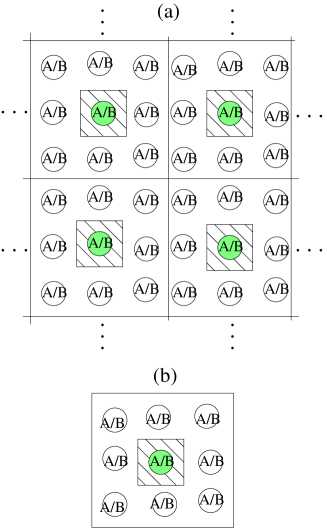
Figure 1: (Color on line)(a) and (b) Show dividing a two dimension square real lattice in to similar super-cells of $N_{c}=9$ with original lattice symmetry around their own central sites. The green color sites illustrate central sites of super-cells and hatched squares show the Wigner-Seitz unite cell (WSUC) of each super-cell of this lattice. The WSUC and super-cells have whole original lattice symmetry around their origins. The super-cell vectors are ${\bf r}_{sc}=ma{\bf e}_{x}+na{\bf e}_{y}$ where $m,n=-1,0,1$ and a is lattice constant. By translate each WSUC with respect to super-cell vectors ${\bf r}_{sc}=ma{\bf e}_{x}+na{\bf e}_{y}$, whole super-cell is cover with out overlapping. (c) and (d) show this 2d lattice divided in to four site clusters, $N_{c}=4$, where non of these clusters preserve original lattice symmetry around their own sites.

Since for each lattice vector there is a unique wave vector in the FBZ in the k-space, so for the set of super-cell vectors set $\{{\bf r}_{sc}\}$ it must exist a unique set of super-cell wave vectors in the k-space in the FBZ. To see lattice symmetry effect on the super-cell wave vectors, we reexamine the super-cell wave vectors corresponding to Fig.1 (a) and (c). Fig.2 shows unique super-cell wave vector sets corresponding to nine sites approximation, $N_{c}=9$, of Fig.1 (a).

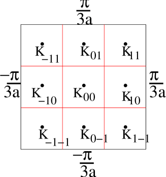
Figure 2: (Color on line) Show FBZ of a 2d square lattice and its cells corresponding to super-cell with $N_{c}=9$. The unique set of super-cell wave vectors are ${\bf K}_{mn}=m\frac{\pi}{3a}{\bf e}_{x}+n\frac{\pi}{3a}{\bf e}_{y}$ where m and n take -1, 0 and 1. All these wave vectors are in the FBZ and the super-cell wave vectors, ${\bf K}$, have full FBZ symmetry around origin ${\bf K}={\bf 0}$

While for the four sites super-cell which is not preserved lattice symmetry, Fig.1 (c), there are four different super-cell wave vector sets as illustrated in Fig.3. The super-cell wave vectors of each set are not preserve FBZ symmetry. Hence we found just super-cells with original lattice symmetry around their own central sites preserve a one to one corresponding between real space super-cell vectors and super-cell wave vectors in the k-space. Therefore in the next part of this section we reformulate the EMSCA for super-cells with lattice symmetry.

     

     

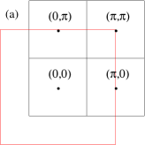
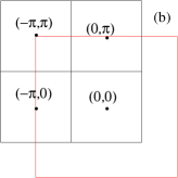
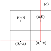
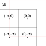
Figure 3: (Color on line) Show four different super-cell wave vector sets $\{(0,0),(0,\pi),(\pi,0),(\pi,\pi)\}$, $\{(0,0),(0,\pi),(-\pi,0),(-\pi,\pi)\}$, $\{(0,0),(\pi,0),(0,-\pi),(\pi,-\pi)\}$ and $\{(0,0),(-\pi,0),(-\pi,-\pi),(0,-\pi)\}$ corresponding to four sites cluster approximation of Fig.1 (c). The red square illustrate FBZ. Non of these cluster wave vector sets are in the FBZ and the super-cell wave vectors, ${\bf K}$, haven’t FBZ symmetry around origin ${\bf K}={\bf 0}$. $a=1$ is the lattice constant.

Since the super-cells in the real lattice are similar, intra super-cell multiple scattering kept and inter super-cell multiple scattering are neglected, hence the super-cell self energy, $\Sigma_{sc}(I,J)$, obey periodicity condition of the original lattice super-cellsMoradian06 ,

$$\Sigma_{sc}({\bf r}_{IJ}+{{\bf L}^{mn}_{sc}})=\Sigma_{sc}({\bf r}_{IJ})$$ (10)

where ${\bf L}^{mn}_{sc}$ is a vector connects central lattice sites of mth and nth super-cells,

$${\bf L}^{mn}_{sc}=\sum_{i}(n_{i}-m_{i})N^{i}_{sc}{\bf a}_{i}$$ (11)

where $m_{i}$ and $n_{i}$ are integer numbers and $N^{i}_{sc}$ is number of lattice sites along the ith primitive vector ${\bf a}_{i}$. So $N^{i}_{sc}{\bf a}_{i}$ is length of super-cell along the ${\bf a}_{i}$ and for a 3-dimension system, number of sites in a super-cell is $N_{sc}=N^{1}_{sc}N^{2}_{sc}N^{3}_{sc}$. $m_{i}-n_{i}=l_{i}$ is an integer number. By applying Eqs.10 and 11 to the following exact self energy relations,

$$\Sigma(I,J)=\frac{1}{N}\sum_{\bf q}\Sigma({\bf q})e^{i{\bf q}.{\bf r}_{IJ}}$$ (12)

we have

$$\sum_{\bf q}\Sigma_{sc}({\bf q})e^{i{\bf q}.({\bf r}_{IJ}+{{\bf L}^{mn}_{sc}})}=\sum_{\bf q}\Sigma_{sc}({\bf q})e^{i{\bf q}.{\bf r}_{IJ}}.$$ (13)

where Eq.13 imply that,

$$e^{i{\bf q}.{{\bf L}^{mn}_{sc}}}=1$$ (14)

hence,

$${\bf q}.{{\bf L}^{mn}_{sc}}=2\pi m^{\prime}$$ (15)

where m’ is an integer number. Eq.15 for the nearest neighbour super-cells, $n_{i},m_{i}=0,1$, defines a unique set of $N_{sc}$ super-cell wave vectors in the first Brillouin zone (FBZ) which have FBZ symmetry around ${\bf K=0}$. To avoid confusing them with the lattice wave vectors k, they are denoted by ${\bf K}=\{K_{n}\}$,

$${\bf K}.{{\bf L}_{sc}}=2\pi m^{\prime}$$ (16)

where ${\bf L}_{sc}=\sum_{i}n_{i}N^{i}_{sc}{\bf a}_{i}$. From Eq.16 for each super-cell size we can obtain super-cell wave vector set $\{{\bf K}_{n}\}$. It should be emphasize that the super-cell wave vectors set, $\{{\bf K}_{n}\}$, around center of FBZ have original FBZ symmetry due to original lattice symmetry of super-cell. To reexamine this method we consider a limit case, when each super-cell extended to the whole lattice, that is $N^{i}_{sc}=N^{i}$, hence $N_{sc}=N$ and ${\bf L}_{sc}={\bf L}$. So the translation vector between nearest neighbour super-cells, where each super-cell are included whole lattice sites, are

$${\bf L}=\sum_{i}n_{i}N^{i}{\bf a}_{i}.$$ (17)

Eq.16 by considering Eq.17 converts to the following periodicity condition

$${\bf K}_{(N_{sc}\rightarrow N)}.{\bf L}=2\pi m^{\prime}.$$ (18)

The super-cell wave vectors set ${\bf K}_{(N_{sc}\rightarrow N)}$ defined by Eq.18 are exactly the lattice vectors ${\bf k}$ defined by the following periodicity Born von Karman condition,

$${\bf k}.{\bf L}=2\pi m^{\prime}$$ (19)

hence in this limit ${\bf K}_{(N_{sc}\rightarrow N)}={\bf k}$ and EMSCA become exact.

In the next part of this section by applying EMSCA to the exact system we drive relation between real space and K-space super-cell self energies, average Green functions and the orthogonality relation. First we investigate self energies. In the EMSCAMoradian06 just self energy inside of each super-cell sites are non zero,

$$\Sigma(i,j)=\delta_{iI}\delta_{jJ}\Sigma_{sc}(I,J)$$ (20)

where I and J are restricted to the same super-cell. We apply Eq.20 to the following exact relation to find relation between K-space and real space super-cell self energies, $\Sigma_{sc}({\bf K}_{n})$ and $\Sigma_{sc}(I,J)$,

$$\Sigma({\bf k})=\frac{1}{N}\sum_{ij}\Sigma(i,j)e^{i{\bf r}_{ij}.{\bf k}}.$$ (21)

Since number of super-cells in the whole lattice is $\frac{N}{N_{sc}}$ and in the super-cell approximation just self energies inside of each super-cell, $\Sigma_{sc}(I,J)$, are nonzero hence by using Eqs.10 and 16, Eq.21 reduces to,

$$\Sigma_{sc}({\bf K}_{n})=\frac{1}{N_{sc}}\sum_{IJ}\Sigma_{sc}(I,J)e^{i{\bf r}_{IJ}.{\bf K}_{n}}.$$ (22)

By converting Eq.22 to the real space we have

$$\sum_{{\bf K}_{n}}\Sigma_{sc}({\bf K}_{n})e^{-i{\bf r}_{I^{{}^{\prime}}J^{{}^{\prime}}}.{\bf K}_{n}} =$$ (23)

$$\frac{1}{N_{sc}}\sum_{IJ}\Sigma_{sc}(I,J)\sum_{{\bf K}_{n}}e^{i({\bf r}_{IJ}-{\bf r}_{I^{\prime}J^{\prime}}).{\bf K}_{n}}$$

where by consider the following super-cell orthogonality condition

$$\frac{1}{N_{sc}}\sum_{{\bf K}_{n}}e^{i{\bf r}_{IJ}.{\bf K}_{n}}=\delta_{IJ}$$ (24)

Eq.III reduces to,

$$\Sigma_{sc}(I,J)=\frac{1}{N_{sc}}\sum_{{\bf K}_{n}}\Sigma_{sc}({\bf K}_{n})e^{-i{\bf r}_{IJ}.{\bf K}_{n}}$$ (25)

Eqs.22, 24 and 25 are a set of equations that can convert real space $\Sigma_{sc}({\bf K}_{n})$ and K-space super-cell self energies $\Sigma_{sc}(I,J)$. Although relation between real space exact self energy,$\Sigma(i,j;E)$, and super-cell self energy, $\Sigma_{sc}(I,J;E)$, is known using Eq.20 but in the K and k-spaces it should clarify. To find relation between exact self energy $\Sigma({\bf k})$ and super-cell self energy $\Sigma_{sc}({\bf K}_{n})$ we defining ${\bf k}={\bf K}_{n}+{\bf k}^{{}^{\prime}}$, where ${\bf k}^{{}^{\prime}}$ restricted to a sub-cell in the FBZ symmetry around super-cell vector ${\bf K}_{n}$. Hence in following exact self energy relation,

$$\Sigma({\bf r}_{IJ})=\frac{1}{N}\sum_{\bf k}\Sigma({\bf k})e^{i{\bf r}_{IJ}.{\bf k}}$$ (26)

the summation over k could be separated in to two parts, $\sum_{\bf k}=\sum_{{\bf K}_{n}}\sum_{{\bf k}^{{}^{\prime}}}$, where k’ are wave vectors with respect to ${\bf K}_{n}$Moradian06 hence,

$$\Sigma({\bf r}_{IJ})=\frac{1}{N}\sum_{{\bf K}_{n}}e^{i{\bf r}_{IJ}.{\bf K}_{n}}\sum_{{\bf k}^{{}^{\prime}}}\Sigma({\bf K}_{n}+{\bf k}^{{}^{\prime}})e^{i{\bf r}_{IJ}.{\bf k}^{{}^{\prime}}}$$ (27)

this exact self energy, $\Sigma(I,J)$, could be convert to the super-cell self energy, $\Sigma_{sc}(I,J)$, if we assume

$$e^{i{\bf k}^{{}^{\prime}}.{\bf r}_{IJ}}=1$$ (28)

and

$$\sum_{{\bf k}^{{}^{\prime}}}\Sigma({\bf K}_{n}+{\bf k}^{{}^{\prime}})=\frac{N}{N_{sc}}\Sigma_{sc}({\bf K}_{n}).$$ (29)

Hence we have

$$\Sigma_{sc}({\bf r}_{IJ})=\frac{1}{N_{sc}}\sum_{{\bf K}_{n}}e^{i{\bf r}_{IJ}.{\bf K}_{n}}\Sigma_{sc}({\bf K}_{n})$$ (30)

Note that similar to Eqs.28 and 29 are introduce in the DCAHettler98 ; Jarrell01 ; Jarrell01-2 . Our next task is to find such relations for Green functions.

To find relation between average super-cell Green function ${\bar{G}}({\bf K}_{n})$ and exact average Green function ${\bar{G}}({\bf k})$,

$${\bar{G}}(I,J)=\frac{1}{N}\sum_{\bf k}{\bar{G}}({\bf k})e^{i{\bf r}_{IJ}.{\bf k}}$$ (31)

where ${\bar{G}}({\bf k})$ is

$${\bar{G}}({\bf k})=(G^{-1}_{0}({\bf k})-\Sigma({\bf k}))^{-1}$$ (32)

and $G^{-1}_{0}({\bf k})$ is bare system Green function. Now we write each wave vector ${\bf k}$ in terms of its nearest super-cell wave vector ${\bf K}_{n}$ and inside cell wave vector ${\bf k}^{\prime}$, ${\bf k}$=${\bf K}_{n}$+${\bf k}^{\prime}$ hence $\sum_{\bf k}=\sum_{{\bf K}_{n}}\sum_{{\bf k}^{{}^{\prime}}}$. By using these and Eq.28 the exact average Green function ${\bar{G}}(I,J)$ in terms of k-space Green function ${\bar{G}}({\bf k})$ is given by,

$${\bar{G}}(I,J)=\frac{1}{N}\sum_{{\bf K}_{n}}\sum_{\bf k^{\prime}}{\bar{G}}({\bf k})e^{i{\bf r}_{IJ}.{\bf K}_{n}}e^{i{\bf r}_{IJ}.{\bf k^{\prime}}}$$ (33)

by using Eq.28 the exact average Green function, ${\bar{G}}(I,J)$, converts to super-cell Green function, ${\bar{G}}_{sc}(I,J)$,

$${\bar{G}}_{sc}(I,J)=\frac{1}{N}\sum_{{\bf K}_{n}}e^{i{\bf r}_{IJ}.{\bf K}_{n}}\sum_{\bf k^{\prime}}{\bar{G}}({\bf K}_{n}+{\bf k^{\prime}})$$ (34)

where relation between K-space super-cell Green function, ${\bar{G}}({\bf K}_{n})$, and k-space exact average Green function, ${\bar{G}}({\bf k})$, is given by,

$$\sum_{\bf k^{\prime}}{\bar{G}}({\bf K}_{n}+{\bf k^{\prime}})=\frac{N}{N_{sc}}{\bar{G}}_{sc}({\bf K}_{n}).$$ (35)

similar to this equation derived in the DCA formalismHettler98 ; Jarrell01 ; Jarrell01-2 . So relation between K-space and real space super-cell Green functions is given by,

$${\bar{G}}_{sc}(I,J)=\frac{1}{N_{sc}}\sum_{{\bf K}_{n}}e^{i{\bf r}_{IJ}.{\bf K}_{n}}{\bar{G}}_{sc}({\bf K}_{n})$$ (36)

To complete our set of equations for calculation self energy and Green function, we apply the EMSCA formalism to the self energy definition equation, Eq.8, where we take average over all super-cells except one, called impurity super-cell, hence the random potentials in all super-cells except impurity super-cell are replace by super-cell self energiesMoradian06 ,

$$\mbox{\boldmath$\varepsilon$}{\bf\rightarrow}\left(\begin{array}[]{ccccc}&\vdots&\vdots&\vdots&\\ ...&{\bf\Sigma}_{sc}&{\bf\Sigma}_{sc}&{\bf\Sigma}_{sc}&...\\ ...&{\bf\Sigma}_{sc}&\mbox{\boldmath$\varepsilon$}_{sc}&{\bf\Sigma}_{sc}&...\\ ...&{\bf\Sigma}_{sc}&{\bf\Sigma}_{sc}&{\bf\Sigma}_{sc}&...\\ &\vdots&\vdots&\vdots&\\ \end{array}\right).$$ (37)

Figure 4 illustrate the EMSCA formalism for a 1d alloy system.

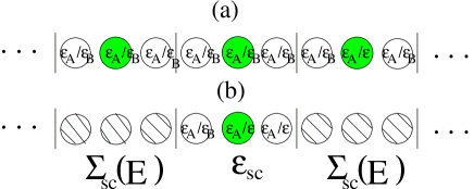
Figure 4: (color on line) Show effective medium super-cell approximation method for a 1d alloy system. (a) Real 1d alloy system divided in to similar three sites super-cells, $N_{c}=3$ where each super-cell have full original lattice. The green color sites illustrate central sites of super-cells. By taking average over all super-cells except one where called impurity super-cell we have one impurity super-cell in an effective medium, where medium constructed from replacing super-cell impurities by super-cell self energies. (b) A super-cell with 3 sites, $N_{c}=3$, in an effective medium super-cell approximation.

Therefore Eq.8 in the EMSCA reduces to,

$$\langle\mbox{\boldmath$\varepsilon$}_{sc}{\bf G}^{imp}_{sc}\rangle_{sc-imp}={\bf\Sigma}_{sc}\bar{{\bf G}}_{sc}.$$ (38)

By inserting Eq.38 in to Eq.9 this equation reduces to the following relation for the super-cell impurity Green function for any arbitrary lattice sites i and j,

$$G^{imp}_{sc} (i,j;E)=\bar{G}_{sc}(i,j;E)+$$

$$\sum_{LL^{\prime}} \bar{G}_{sc}(i,L;E)(\varepsilon_{L}\delta_{LL^{\prime}}-\Sigma_{sc}(L,L^{\prime};E))\times$$

$$G^{imp}_{sc}(L^{\prime},j;E).$$

When i and j restrict to impurity super-cell sites, Eq.LABEL:eq:general_super-cell_random-green reduces to,

$$G^{imp}_{sc} (I,J;E)=\bar{G}_{sc}(I,J;E)+$$

$$\sum_{LL^{\prime}} \bar{G}_{sc}(I,L;E)(\varepsilon_{L}\delta_{LL^{\prime}}-\Sigma_{sc}(L,L^{\prime};E))\times$$

$$G^{imp}_{sc}(L^{\prime},J;E)$$

where

$$\langle G^{imp}_{sc}(I,J;E)\rangle=\bar{G}_{sc}(I,J;E).$$ (41)

Although Eq.LABEL:eq:super-cell_random-green can be separated in to two equations by definition of cavity Green functionMoradian06 but for disorder systems it is not necessary to defined such cavity Green function, although we must defined it in general for interacting disorder systemsMoradian06 . Eqs.35, 36, 38, LABEL:eq:super-cell_random-green and 41 construct a complete set of equations to be solved self consistently to obtain super-cell self energy ,$\Sigma_{sc}(L,L^{\prime};E)$, and average super-cell Green function $\bar{G}_{sc}(I,J;E)$. The algorithm for calculation of average Green function $\bar{G}_{sc}(I,J;E)$ in the EMSCA is as follows

1- A guess for K-space self energies $\Sigma_{sc}({\bf K}_{\bf n})$ usually zero.

2- Calculate the super-cell average K-space Green functions, $\bar{G}({\bf K}_{\bf n})$, by inserting $\Sigma_{sc}({\bf K}_{\bf n})$ in $\bar{G}({\bf K}_{\bf n})=\sum_{\bf k^{\prime}}(G^{-1}_{0}({{\bf K}_{n}}+{\bf k^{\prime}})-\Sigma({\bf K}_{\bf n}))^{-1}$.

3- Fourier transform of K-space $\bar{G}_{sc}({\bf K}_{\bf n})$ to obtained real space Green function $\bar{G}_{sc}(I,J;E)$.

4- Calculate $G^{imp}_{sc}(I,J;E)$ by inserting $\Sigma_{sc}(L,L^{\prime};E)$ and $\bar{G}_{sc}(I,J;E)$ in to Eq.LABEL:eq:super-cell_random-green.

5- Calculate average Green function $\bar{G}_{sc}(I,J;E)$ by using Eq.41 by taking average over all possible impurity configurations.

6- Calculate new self energies $\Sigma_{sc}(L,L^{\prime};E)$ by inserting obtained $G^{imp}_{sc}(I,J;E)$ and $\bar{G}_{sc}(I,J;E)$ in Eq.38.

Now we apply our method to a 1 dimension (1d) alloy system. Since just super-cells with odd number of lattice sites preserve the lattice symmetry with respect to their middle site, we compared calculated average density of states for different super-cell size. Figure5 illustrate average density of states for super-cells $N_{c}=1,\;3,\;7$. By increasing super-cell size more peaks in the average density of states. The corrections are due to nonlocal effects where neglected in the single site approximations, $N_{c}=1$.

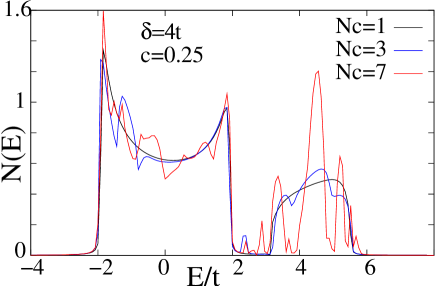
Figure 5: (color on line) Show comparison of average density of states of a 1d alloy system for CPA, $N_{c}=1$, EMSCA with super-cell sizes, $N_{c}=3$ and $N_{c}=7$ where super-cell have original lattice symmetry. The strength length, $\delta=4t$, impurity concentration is $c=0.25$ and $\mu=0$. The difference between DOS are due to nonlocal corrections.

IV Conclusion

We have added an extra condition to the cluster approximations such as Dynamical cluster approximation (DCA), non local coherent potential approximation (NLCPA) and effective medium approximation (EMSCA), where the chosen cluster must have original lattice symmetry with respect to its central site. This condition leads to a one to one correspondence between super-cell sites and super cell wave vectors in the first Brillouin zone hence a unique set of super-cell vectors for each cluster size. One of this vector is ${\bf K}=(0,0,0)$ and other super-cell vectors around this vector have full FBZ symmetry. While without this condition, for some cluster sizes, some of the cluster wave vectors locating in the higher Brillouin zones. This lead to two effects, first asymmetry of cluster wave vectors with respect to FBZ center hence when number of sites in the cluster goes to whole lattice sites the cluster wave vectors are not cover whole FBZ. Second, existence of many set of cluster wave vectors. In our formalism when number of cluster sites goes to number of lattice sites the super-cell vectors recover whole FBZ and EMSCA become exact.

References

• (1) P. Soven, Phys. Rev. B , 156, 809 (1967).
• (2) M. H. Hettler, A. N. Tahvildar-Zadeh, M. Jarrell, T. Pruschke, and H. R. Krishnamurthy, Phys. Rev. B 61, 12739 (1998).
• (3) M. Jarrell, Th. Maier, C. Huscroft and S. Moukouri, Phys. Rev. B 64, 195130 (2001).
• (4) M. Jarrell and H. R. Krishnamurthy, Phys. Rev. B 63, 125102 (2001).
• (5) Rostam Moradian, Balazs. L. Györffy, James. F. Annett, Phys. Rev. Lett. 89, 287002 (2002).
• (6) R. Moradian, Phys. Rev. B 70, 205425 (2004).
• (7) R. Moradian, J. Phys: Condens. Matter 18, 507 (2006).
• (8) D. A. Rowlands, X.-G. Zhang, Phys. Rev. B 78, 115119 (2008).
• (9) Neil W. Ashcroft and N. David Mermin, Solid State Physics, HRW International Edition, Hong Kong (1987).
• (10) J. M. Ziman, Models of Disorder (Cambridge University Press, Cambridge, England, 1979).