Abstract

When an infectious disease strikes a population, the number of newly reported cases is often the only available information during the early stages of the outbreak. An important goal of early outbreak analysis is to obtain a reliable estimate for the basic reproduction number, ${\mathcal{R}}_{0}$.

Over the past few years infectious disease epidemic processes have gained attention from the physics community. Much of the work to date, however, has focused on the analysis of an epidemic process in which the disease has already spread widely within a population; conversely, very little attention has been paid, in the physics literature or elsewhere, to formulating the initial phase of an outbreak. Careful analysis of this phase is especially important as it could provide policymakers with insight on how to effectively control an epidemic in its initial stage.

We present a novel method, based on priciples of network theory, that enables us to obtain a reliable real-time estimate of the basic reproduction number at an early stage of an outbreak. Our method takes into account the possibility that the infectious period has a wide distribution and that the degree distribution of the underlying contact network is heterogeneous. We validate our analytical framework with numerical simulations.

Introduction

The basic reproduction number, ${\mathcal{R}}_{0}$, is a fundamental characteristic of the spread of an infectious disease. It is generally defined as the expected number of new infections caused by a typical individual during the entire period of his/her infection in a totally susceptible population [1, 2, 3]. Because ${\mathcal{R}}_{0}$ is a simple scalar quantity, and perhaps because in many circumstances it determines the expected (average) final size of an outbreak [4, 3, 5, 6, 7], it has been widely used to gauge the degree of threat that a specific infectious agent will pose as an outbreak progresses [8, 9, 10]. While it is clear that knowing the value of ${\mathcal{R}}_{0}$ can be very useful for policymakers in planning a response; it is not as straightforward to obtain a reliable estimate of ${\mathcal{R}}_{0}$, especially in early stages of an outbreak, before large scale uncontrolled transmission has taken place and before the basic biology and transmission pathways of the pathogen have been characterized.

Early in an outbreak, the pattern of disease spread is predominantly influenced by the probabilistic nature of infection transmission. Consequently, a wide array of outcomes is possible, ranging from the outbreak fizzling out, even in the absence of an intervention, to circumstances where the initial stage expands into a large-scale epidemic. Once a full-blown epidemic develops, several assumptions can be made that simplify the estimation of ${\mathcal{R}}_{0}$, as has been discussed in detail in the literature [1, 3, 8, 5].

In many cases, it is necessary to assess the impact of various intervention strategies before a large-scale epidemic occurs. In doing so, stochastic manifestations of disease transmission as well as the underlying structure of the contact network should be taken into account. The first aspect has been widely studied. For example, the Reed-Frost model is a chain-binomial stochastic model where each infected individual can infect susceptible individuals and they are all assumed to have the same contact rate [11, 12, 13, 14]. Another example is the methodology developed by Becker [15], and Ball and Donnelly [16] based on a branching process susceptible-infected-recovered (SIR) model. Branching processes have received wide attention because they facilitate the evaluation of the basic reproduction number as well as the final epidemic size and epidemic probability [17]. More recently, the 2003 global outbreak of severe acute respiratory syndrome (SARS) inspired the development of new methodologies based on the daily number of new cases and the distribution of the serial interval between successive infections [18, 19, 20, 21]. However, none of these methods take into consideration the influence of the contact network underlying an epidemic process or it is assumed that the contact network is a classic random graph.

Several new methods to estimate the basic reproduction number, ${\mathcal{R}}_{0}$, were proposed during or shortly after the 2009 H1N1 influenza pandemic. Notably, Nishiura et al.[22] employed an age-structured model to derive an estimate for ${\cal R}_{0}$. Katriel et al.[23] used a new discrete-time stochastic epidemic SIR model that explicitly takes into account the disease’s specific generation-time distribution and the intrinsic demographic stochasticity inherent to the infection process. Balcan et al. [24] employed a method that is based on the distribution of arrival times of the H1N1 in 12 different countries seeded by the Mexico epidemic using one million computationally simulated epidemics. Nishiura et al. [25] also developed a discrete time stochastic model that accounts for demographic stochasticity and conditional measurement and applied to estimate the ${\cal R}_{0}$ value using the weekly incidence of H1N1 pandemic influenza in Japan. Although all of these constitute an important advancement in the literature, none of them simultaneously addresses analytically the stochasticity due to the underlying contact network and the transmission process.

Outline Summary

In the following we first describe the basic notion of network model. We then define infection hazard or infectivity function, the removal hazard or removal function and their related quantities namely the transmissibility and the removal probability density function. Furthermore, we derive a stochastic renewal equation that allows us to understand the relationship between the rate of newly-infected individuals at a given time and all preceding infected cases in the initial stage of an outbreak. We study the renewal equation in the exponential regime and obtain the Wallinga-Lipsitch equation[26]. In this regime, we also obtain an equation that express the generation interval distribution in term of the transmissibility and the removal probability distribution function. In next part, we obtain an equation for the basic reproduction of removed individual. This equation acts as a constrain allowing us to find one unknown. We will then draw an algorithm and show how one can evaluate the basic reproduction number. We finally present our extensive numerical results showing the accuracy of the methodology in predicting the basic reproduction number for different network models and parameters types and values.

Network basis

This section briefly introduces the idea of contact network epidemiology and defines the key concepts of infection rate, removal rate, transmissibility and removal probability density. We map a collection of $N$ individuals to a network where each vertex represents an individual and each edge shows a pathway of possible infection transmission between two individuals. We use $k$ to denote the degree of a given individual (the number of contacts that s/he has) represented graphically by the number of edges emanating from a vertex, and we use $p_{k}$ to denote the degree distribution (the probability that a randomly chosen vertex has degree $k$ ($k$ contacts)). Several important quantities can be derived once a network’s degree distribution is known. The moments of the degree distribution are $\langle k^{n}\rangle=\sum_{\kappa=0}^{\infty}k^{n}p_{\kappa}$. For $n=1$, $\langle k\rangle$ is the average number of nearest neighbours of a randomly chosen individual, which we denote $z_{1}$. The average number of second nearest neighbours of a randomly selected individual, $z_{2}$, can be expressed as $\langle k^{2}\rangle-\langle k\rangle$ [27]. To estimate ${\mathcal{R}}_{0}$, we count the number of edges along which an individual can infect others, once that individual has become infected. This quantity, usually termed excess degree, represents the number of edges emanating from a vertex (individual), excluding the edge that was the source of the infection. One can show that the average excess degree ($Z_{x}$) is given by the ratio $\frac{z_{2}}{z_{1}}$ [29].

We denote the time at which an individual acquires the infection by $t_{i}$, and the time since acquiring infection by $\tau=t-t_{i}$ (also known as age of infection). While harbouring the infection, the individual is first latent (infected but not yet infectious) and then infectious (either symptomatically or asymptomatically). The individual may also recover, by which we mean only that s/he can no longer transmit the infection, not that s/he has necessarily completely cleared the pathogen. For some diseases, after a temporary recovery, the person may become infectious again. Knowing that an individual acquires infection at a given time $t_{i}$, various states of infectiousness for this individual can be encapsulated within the infection hazard or infectivity function, $\lambda_{i}(\tau)$. The infectivity function measures the instantaneous risk of disease transmission across an edge. This implies that for small $\delta\tau$ the conditional probability that infection occurs across an edge between times $\tau$ and $\tau+\delta\tau$, given that it did not occur by time $\tau$, can be approximated by $\lambda_{i}(\tau)\delta\tau$. Typically, $\lambda_{i}(\tau)$ is initially zero during the latent period, it increases to a certain level and then declines during the infectious period, before finally vanishing and returning to zero at the time of permanent recovery. Figure 1 shows four hypothetical infectivity functions, the first of which is the typical case. In practice, the functional form of $\lambda_{i}(\tau)$ should be estimated from the actual transmission profile corresponding to a specific disease. Note that the only technical restriction on $\lambda_{i}(\tau)$ is that it must be a non-negative integrable function.

Figure 1: Hypothetical infectivity functions, $\lambda_{i}(\tau)$. They show the general infectivity patterns that can occur, varying by complexity of the disease. Top left panel shows the infectivity function of a very generic disease, top right panel shows the infectivity function of an HIV type disease, bottom left displays the infectivity function of any recurrent disease such as chicken-pox and finally bottom right panel exhibits the infectivity function an influenza type disease.

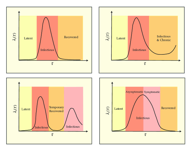
Given the infectivity function, one can evaluate the probability that an individual transmits the disease to one of his/her contacts during a specific time period. Let $T(\tau)$ denote the probability of disease transmission along one edge for an individual with infection age $\tau$. Then $T(\tau)$ satisfies [30, 27]

$$T(\tau)=1-\exp\left(-\int_{0}^{\tau}\lambda_{i}(\tau^{\prime})d\tau^{\prime}\right).$$ (1)

In general, the time-to-removal varies from one individual to another and there is no a priori knowledge of the exact value of this quantity for each individual. Therefore we must account for its variability as well. Let $\lambda_{r}(\tau)$ denote the removal hazard or removal function, i.e., the instantaneous rate of removal for an individual with infection age $\tau$. This implies that for small $\delta\tau$ the conditional probability that an individual is removed between times $\tau$ and $\tau+\delta\tau$, given that s/he was not removed by time $\tau$, can be approximated by $\lambda_{r}(\tau)\delta\tau$. The removal function indicates how quickly the infectious individuals are removed from disease dynamics as a function of the duration of their infection. This can be related to death or various interventions, such as quarantine, reduction of social activity due to severity of illness, behaviour change etc. Let $\Psi(\tau)$ denote the probability that an individual has time-to-removal $\geq\tau$. Then [30]

$$\Psi(\tau)=\exp\left(-\int_{0}^{\tau}\lambda_{r}(\tau^{\prime})d\tau^{\prime}\right),$$ (2)

subject to the condition $\Psi(\infty)=0$. The removal probability density function is given by $\psi(\tau)=-\frac{d\Psi(\tau)}{d\tau}$ (or $\Psi(\tau)=\int_{\tau}^{\infty}\psi(\tau^{\prime})d\tau^{\prime}$).

Using Equation (1) and $\psi(\tau)$ (or $\Psi(\tau)$) one can calculate the expected transmissibility, i.e the probability of disease transmission - across a given edge:

$$T = \int_{0}^{\infty}\psi(\tau)T(\tau)d\tau=\int_{0}^{\infty}\Psi(\tau)\frac{dT(\tau)}{d\tau}d\tau$$ (3)

$$= \int_{0}^{\infty}{\lambda_{r}(\tau)e^{-\int_{0}^{\tau}\lambda_{r}(u)du}[1-e^{-\int_{0}^{\tau}\lambda_{i}(u)du}]d\tau}.$$

The basic reproduction number, which represents the average number of infections caused by a typical infected individual in a fully susceptible population, can be written as the product of the expected excess degree and the expected transmissibility [27]

$${\mathcal{R}}_{0}=Z_{x}T.$$ (4)

Disease dynamics on networks

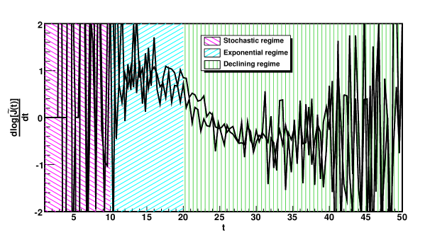
In this section we present some examples of the spread of an infectious agent on a contact network. The pattern of disease spread on a network can be categorized into three different regimes: stochastic, exponential and declining. The process of disease spread is stochastic in nature, given that the disease transmission along an edge occurs in a probabilistic manner and that the degree of the next infected individual cannot be determined a priori. The stochastic behaviour is dominant in the initial stage of disease spread when the number of infectious individuals is comparatively small (stochastic regime). The effect of stochasticity becomes much less pronounced when the number of newly infected individuals becomes significant, and stochastic fluctuations are smoothed out (exponential regime). Progression of disease spread starts to decline as the cumulative number of infected cases becomes comparable to the size of the network, at which point network finite-size effects becomes important (declining regime)[29].

From now on, we use the tilde notation to make the distinction between the realization of a stochastic process (with tilde) and its mean field value (without tilde). We define $\tilde{j}(t)$ as the time series of infection events, which is a sum of delta Dirac functions located at each infection time. The case count $\tilde{C}(t,\delta t)$ that gives the number of infections between times $t$ and $t+\delta t$ can be expressed as $\tilde{C}(t,\delta t)=\int_{t}^{t+\delta t}\tilde{j}(t^{\prime})dt^{\prime}$. We define $\tilde{J}(t)=\tilde{C}(t,\delta t)/\delta t$ as the incidence rate of new infections at time $t$, where $\delta t$ is the maximum time resolution. In the exponential regime, the incidence rate of new infections grows exponentially and therefore can be expressed as:

$$\tilde{J}(t)\simeq J_{0}\exp(\alpha t),$$ (5)

for some $\alpha>0$. The above-mentioned regimes are represented in Figure 2.

Figure 2: Two hypothetical realizations of an epidemic process on a network. The left, middle and right represent stochastic, exponential and declining regimes, respectively.

Stochastic dynamics of disease

In this section we outline a general framework to estimate the basic reproduction number assuming that all information about a specific realization of the epidemic process up to time $t$ is known. We start by first deriving a renewal equation for the rate of new infections, $\tilde{J}(t)$.

A renewal equation for $\tilde{J}(t)$

Let’s consider the first person in the population infected with the disease and assume that her/his infection occurred at time $0$. From equation (3), we can infer that the expected number of infections that this individual will cause by time $t$ is given by

$$Z_{x}\int_{0}^{t}\Psi(\tau)\frac{dT(\tau)}{d\tau}d\tau$$ (6)

(assuming that his/her excess degree is equal to the average excess degree). This leads in the limit $t\rightarrow\infty$ to the usual value of ${\cal R}_{0}=Z_{x}T$. The above expression also implies that the mean contribution of this individual to the incidence rate of new infections at his/her infection age $\tau$ is given by

$$Z_{x}\Psi(\tau)\frac{dT(\tau)}{d\tau}.$$ (7)

The above equations can be readily generalized to address the random process of infection spread on a contact network. In particular, one can compute the contribution of the individuals infected at time $t-\tau$, $\tilde{J}(t-\tau)\delta t$, to the number of new infections occurring in initial stage of an outbreak at time $t$, $\tilde{J}(t)\delta t$, namely

$$\tilde{J}(t)\delta t=Z_{x}\int_{0}^{t}\tilde{J}(t-\tau)\delta t\Psi(\tau)\tilde{\Theta}(\tau,t)d\tau.$$ (8)

where $\tilde{\Theta}(\tau,t)$ denotes the fraction of those edges where disease is actually transmitted exactly at time $t$. This is a random function with expectation given by $\frac{dT(\tau)}{d\tau}$. Please note that $Z_{x}$ and $\Psi(\tau)$ are a function of $t$ in the most general case. Expression (8) is a generalization of the classical Lotka renewal equation for population growth [31, 32], here applied to epidemic dynamics when taking into account the structure of the underlying contact network and the stochasticity inherent to the transmission process.

Exponential regime and the generation interval distribution

In this section we show the relationship between our results and the methodology developed by Wallinga and Lipsitch [26]. During the exponential regime we can ignore stochastic fluctuations and replace all quantities with their expected values. In particular, if we ignore stochastic effects we can re-write the renewal equation (8) as

$$J(t)=Z_{x}\int_{0}^{t}J(t-\tau)\Psi(\tau)\frac{dT(\tau)}{d\tau}d\tau$$ (9)

where we used $\tilde{\Theta}(\tau,t)\approx\frac{dT(\tau)}{d\tau}$.

Let $\chi(\tau)\equiv Z_{x}\Psi(\tau)\frac{dT(\tau)}{d\tau}$. Equation (9) then takes the simpler form

$$J(t)=\int_{0}^{t}J(t-\tau)\chi(\tau)d\tau,$$ (10)

which is the well-known Lotka renewal equation [31, 32].

From the definitions of $\chi(\tau)$, the expected transmissibility (Eq. (3)) and the basic reproduction number (Eq. (4)) we can see that $\int_{0}^{\infty}\chi(\tau)d\tau={\mathcal{R}}_{0}$. Substituting $J(t)\approx\exp(-\alpha t)$ in Eq. (10) and taking the limit when $t\rightarrow\infty$ we obtain that

$$1=\int_{0}^{\infty}\exp(-\alpha\tau)\chi(\tau)d\tau.$$ (11)

It is worth mentioning that the exact exponential regime can be reached when $t\rightarrow\infty$ for an infinite-size network and that is why it is valid to take the limit. This means that there should be a slight deviation from the exponential behaviour for a “finite-size” system at “finite time” once the outbreak has surpassed the stochastic regime. Dividing both sides of Eq. (11) by ${\mathcal{R}}_{0}$ we find that [26]

$$\frac{1}{{\mathcal{R}}_{0}}=\int_{0}^{\infty}\exp(-\alpha\tau)\hat{\chi}(\tau)d\tau,$$ (12)

where $\hat{\chi}(\tau)=\chi(\tau)/{\mathcal{R}}_{0}$ is defined as the generation interval distribution. This equation relates the basic reproduction number to the Laplace transform of the generation interval distribution in the asymptotic case (infinite-size, infinite-time). Now, in our formulation the generation interval distribution can be written as

$$\hat{\chi}(\tau)=\frac{\Psi(\tau)\frac{dT(\tau)}{d\tau}}{\int_{0}^{\infty}\Psi(\tau^{\prime})\frac{dT(\tau^{\prime})}{d\tau^{\prime}}d\tau^{\prime}}.$$ (13)

This equation describes how the transmissibility, $T(\tau)$, and the distribution of the time to removal, $\Psi(\tau)$, determine together the generation interval distribution.

The generation interval distribution for constant parameters

Equation (11) has a simpler form for constant $\lambda_{r}$ and $\lambda_{i}$. This can be obtained by replacing $\psi(\tau)=\lambda_{r}\exp(-\lambda_{r}\tau)$ and $T(\tau)=1-\exp(-\lambda_{i}\tau)$ inside Equation (11)

$$1 =Z_{x}\lambda_{i}\int_{0}^{\infty}\exp(-\tau\lambda_{r})\exp(-\alpha\tau)\exp(-\lambda_{i}\tau)d\tau$$ (14)

$$=Z_{x}\frac{\lambda_{i}}{\lambda_{i}+\lambda_{r}+\alpha}$$ (15)

or

$$\alpha=\left(Z_{x}-1\right)\lambda_{i}-\lambda_{r}.$$ (16)

Therefore, we can express the rate of exponential growth of an epidemic in terms of the mean excess degree ($Z_{x}$), the infectivity ($\lambda_{i}$) and removal ($\lambda_{r}$) rates.

Furthermore, we can also explicitly compute the generation interval distribution (Eq. (13))

$$\hat{\chi}(\tau)=(\lambda_{i}+\lambda_{r})e^{-(\lambda_{i}+\lambda_{r})\tau}.$$ (17)

For constant parameters the generation interval is an exponential random variable with mean $1/(\lambda_{i}+\lambda_{r})$. Using this fact and Eq. (12) we obtain the following expression for ${\mathcal{R}}_{0}$

$${\mathcal{R}}_{0}=\frac{\lambda_{i}+\lambda_{r}+\alpha}{\lambda_{i}+\lambda_{r}}=1+\frac{\alpha}{\lambda_{i}+\lambda_{r}}.$$ (18)

This equation relates the value of ${\mathcal{R}}_{0}$ to the rate of growth during the exponential phase of an epidemic ($\alpha$) the infection rate ($\lambda_{i}$) and the removal rate ($\lambda_{r}$). Notice that in contrast to the results obtained from a deterministic SIR model, where the mean generation interval is equal to the mean duration of infection [26], here we find that the mean generation interval also depends on the infection rate.

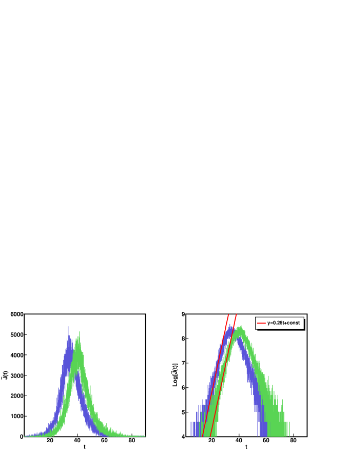
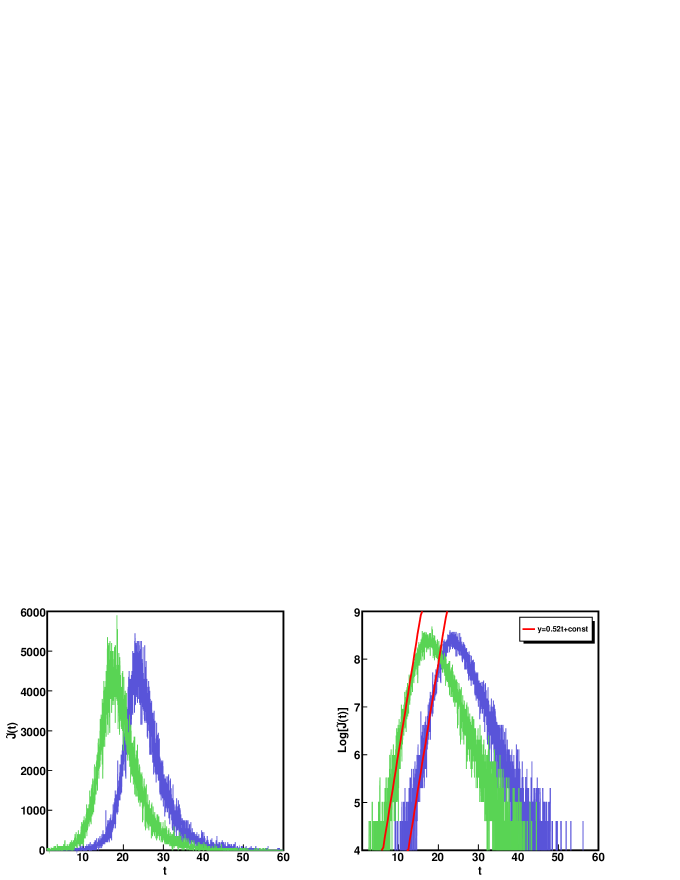
Figures 3 and 4 show two examples of the epidemic behaviour in the three regimes. The algorithm used to simulate the spread of an infectious agent on a contact network is described in the appendix. The left panel of Figure 3 shows two epidemic events unfolding (two different initial index cases) on a binomial network $p_{k}=\left(\begin{matrix}Nk\end{matrix}\right)p^{k}(1-p)^{N-k}$ with $N=100,000$ nodes, $z_{1}=5$ (or $p=z_{1}/(N-1)$), $Z_{x}=5$ and $\{\lambda_{i}=0.12771,\;\lambda_{r}=0.25\}$. Using Equation (3) the expected transmissibility can be calculated as $T=0.338$. The stochastic, exponential and declining regimes are approximately between $0\leq t<20$, $20\leq t<40$ and $40\geq t$ time units, respectively. Also, in the right panel of Figure 3, we show the variation of $Log[\tilde{J}(t)]$ with $\delta t=0.02$ over time. The two solid lines $y_{1},y_{2}=\alpha t+const$ with $\alpha=0.26084$ are the tangent of $Log[\tilde{J}(t)]$ during the exponential regime (Eq.  (16)). This shows the consistency between the simulated epidemic curve and its expected (exponential growth) behaviour. Figure 4 shows the same results for an exponential network with $p_{k}=\left(1-e^{-1/\kappa}\right)e^{-k/\kappa}$, $\kappa=4$, $z1=3.52$, and $Z_{x}=7.0416$. In this example, the stochastic, exponential and declining regimes are approximately between $0\leq t<10$, $10\leq t<20$ and $20\leq t$ time intervals, respectively. The lines $y_{1},y_{2}=\alpha t+const$ with $\alpha=0.52158$ are again the tangent of $Log[\tilde{J}(t)]$ during the exponential regime. Notice that although here we know the “true” value of $\alpha$, in practice it can be estimated from real-life time series data if the outbreak progresses beyond the stochastic regime. As can be seen in Figures 3 and 4 the cases count $\tilde{J}(t)$, generally resembles a typical epidemic curve if the pattern of disease spread has a chance to grow substantially.

Figure 3: The rate of new infections $\tilde{J}(t)$ (left panel) and its logarithm (right panel) for a binomial network with $z_{1}=5$, $\lambda_{i}=0.12771$ and $\lambda_{r}=0.25$. Two independent epidemic realizations are shown in each panel (green and blue). The solid red line shows the tangent of $Log[\tilde{J}(t)]$ in the exponential regime.

Figure 4: The number of newly-infected cases (left panel) and its logarithm (right panel) for an exponential network with $\kappa=4$, $\lambda_{i}=0.12771$ and $\lambda_{r}=0.25$. Two independent epidemic realizations are shown in each panel (green and blue). The solid red line shows the tangent of $Log[\tilde{J}(t)]$ in the exponential regime.

The number of infected and removed individuals at time $t$

Using the quantities introduced in the previous sections, we now derive other expressions that will be helpful in estimating the basic reproduction number, ${\cal R}_{0}$. As an outbreak progresses, at any given time there is a population of infectious individuals, $\tilde{I}(t)$, and a population of removed individuals, $\tilde{R}(t)$. The number of affected individuals - the total number of infected individuals at time $t$ and those who are recovered/removed by time $t$ - is given by

$$\tilde{I}(t)+\tilde{R}(t)=N-\tilde{S}(t)=\int_{0}^{t}\tilde{J}(t-\tau)d\tau,$$ (19)

where $\tilde{S}(t)$ denotes the number of susceptible individuals at time $t$. As illustrated in Figure 5, the total number of infected cases can be written as

$$\tilde{I}(t)=\int_{0}^{t}\tilde{J}^{i}(\tau,t)d\tau=\int_{0}^{t}\tilde{J}(t-\tau)\tilde{\Psi}(\tau)d\tau$$ (20)

which in turn, implies that

$$\tilde{R}(t)=\int_{0}^{t}\tilde{J}^{r}(\tau,t)d\tau=\int_{0}^{t}\tilde{J}(t-\tau)\left[1-\Psi(\tau)\right]d\tau$$ (21)

where $J^{i}(\tau,t)=\tilde{J}(t-\tau)\Psi(\tau)$ and $J^{r}(\tau,t)=\tilde{J}(t-\tau)[1-\Psi(\tau)]$.

Figure 5: This figure illustrates schematically the dependency of the rate of new infections, $\tilde{J}(t)$ (blue curve), on its past values. Only a fraction of the cases infected at time $t-\tau$, $\tilde{J}(t-\tau)\delta t$, contributes to the infections at time $t$, $\tilde{J}^{i}(\tau,t)\delta t=\tilde{J}(t-\tau)\delta t\Psi(\tau)$ (red curve); the rest, $\tilde{J}^{r}(\tau,t)\delta t=\tilde{J}(t-\tau)\delta t[1-\Psi(\tau)]$, have already been removed.

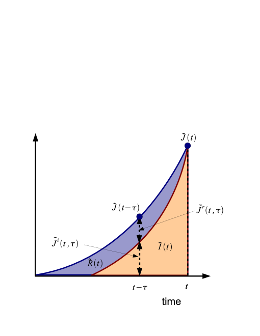
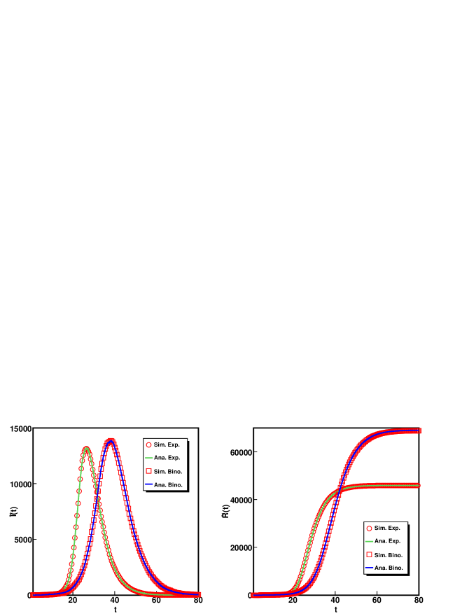
Figure 6 shows the number of infectious (left panel) and removed (right panel) individuals for a disease that spreads either on a binomial or an exponential network. In both panels the curves comprising of red symbols correspond to the computer simulation of an epidemic on the corresponding network; during the simulation the new case counts are recorded to create a synthetic “time series” for $\tilde{J}(t)$. The solid curves correspond to Equations (20) or (21) (for $\tilde{I}(t)$ or $\tilde{R}(t)$) for the corresponding network. These figures show a perfect agreement for both networks between the analytical formulas and the case counts from the simulation.

Figure 6: Number of infectious (left panel) and removed individuals (right panel) as a function of time for the binomial ($z_{1}=5$, $\lambda_{i}=0.12771$ and $\lambda_{r}=0.25$) and exponential ($\kappa=4$) networks. The solid curves come from the evaluation of Equations (20) and (21)), and the symbols from direct counting of the infectious and removed individuals at any given time for a specific realization of the process.

Figure 7: A snapshot of the initial phase of an outbreak starting from the central vertex shown by the purple circle (already removed). The blue/purple, red and green circles represent removed, infectious and susceptible individuals, respectively. The links are presented by lines, those that carried the disease are shown by the arrows. Four different types of pairs (pair of infected individuals) can be easily recognized in this figure and they are shown separately on the right hand side of the figure.

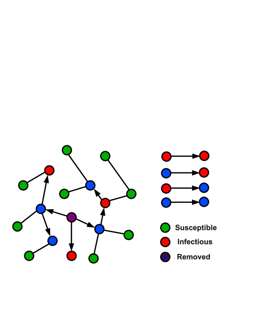
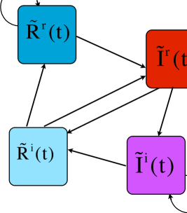
In Figure 7, we show the state of the population during the initial phase of an outbreak starting from the central vertex shown by the purple circle (already removed). The blue/purple, red and green circles represent removed, infectious and susceptible individuals, respectively. The links are presented by lines, those that carried the disease are shown by the arrows. Four different types of pairs (pairs of individuals who have been infected) can be easily recognized in this figure and they are presented on the right side of the figure. These pairs can be collected in four different groups Figure 8 and can be shown by $\tilde{I}^{i}(t)$, $\tilde{I}^{r}(t)$, $\tilde{R}^{i}(t)$ and $\tilde{R}^{r}(t)$, where $R$ and $I$ refer to the number of removed and infectious individuals respectively, with two different predecessors, shown with the superscripts $\{r$,$i\}$ (removed and infectious). Not all groups are necessarily connected to one another. For instance, a recovered/removed predecessor, denoted by superscript $r$ in $\tilde{R}^{r}(t)$, may only come from a group whose members were recovered while their predecessors were still infectious ($\tilde{R}^{i}$), or from a group in which the person and his/her predecessor are removed (denoted by the self-loop from $\tilde{R}^{r}$ to itself). Similarly, the recovered predecessor ($r$) of an infected person ($\tilde{I}^{r}(t)$), may only come from a group of recovered individuals whose respective predecessors were infectious ($\tilde{R}^{i}(t)$) or from a group whose respective predecessors were already recovered ($\tilde{R}^{r}(t)$).

The transmissibility of removed individuals

Our methodology to estimate ${\cal R}_{0}$ is based on a detailed analysis of the characteristics of removed individuals. This is because the history of removed individuals contains all the information about the mechanisms of disease transmission and recovery process. In particular, the period of infection of these individuals can help us estimate the distribution of removal times. Furthermore, since removed individuals have already had the oppertuinity to transmit the disease, the fraction of their contacts that they actually infected contains a lot of information about the transmissibility of disease. In an ideal world, a full characterization of the infection history of each removed individual would be enough to estimate ${\cal R}_{0}$. However, in reality, it is extremely difficult to know which infected individuals have already been removed and what fraction of their potential infections actually occurred. Therefore, we instead derive theoretical expressions that can help us estimate some of these quantities.

First we write an expression for the total number of secondary contacts of those individuals already removed by time $t$. Using ideas similar to those above, the total excess degree of removed individuals can be written as

$$\tilde{{\cal Z}}_{x}^{r}(t)=Z_{x}\int_{0}^{t}\tilde{J}(t-\tau)\left[1-\Psi(\tau)\right]d\tau$$ (22)

Here, $\tilde{{\cal Z}}_{x}^{r}(t)$ represents the total number of edges of already removed individuals that could have transmitted the infection by time $t$. However, only a fraction of these links actually transmitted the disease successfully. This latter fraction is given by $\tilde{I}^{r}(t)+\tilde{R}^{r}(t)$, where $\tilde{I}^{r}(t)$ and $\tilde{R}^{r}(t)$ represent the number of infectious and removed individuals at time $t$, respectively whose predecessor is already removed. The ratio of these two quantities represents the fraction of potential transmissions that actually occurred, which we shall refer to as the expected transmissibility of removed individuals or $\tilde{T}^{r}(t)$.

$$\tilde{T}^{r}(t)\equiv\frac{\tilde{I}^{r}(t)+\tilde{R}^{r}(t)}{\tilde{{\cal Z}}_{x}^{r}(t)}.$$ (23)

Estimates for the expected values for these quantities can, in principle, be calculated based on the rate of new infections, $J(t)$, using arguments similar to those above. These expressions are derived in the next section. Equations (23) and (11) form a set of equations that allows us to find two unknowns, lets say, the amplitude and variance of infectivity profile that is the subject of other study. Here we use equation (23) to solely estimate the basic reproduction number, ${\mathcal{R}}_{0}$.

Figure 8: This figure illustrates various options of causality between infected and recovered cases. The main symbol ($\tilde{I}$ or $\tilde{R}$) denotes the current status of an individual, and the superscript ($i$ or $r$) corresponds to the status of the person who passed the infection on to this individual. $\tilde{I}^{r}(t)+\tilde{R}^{r}(t)$ constitutes the number of infections caused by already removed individuals.

Expression for the transmissibility of removed individuals, $\tilde{T}^{r}(t)$

As discussed in the previous section, our methodology is based on a careful analysis of the characteristics of the removed individuals. In particular, the expected transmissibility of removed individuals, $\tilde{T}^{r}(t)$, will play a crucial role in the estimation of ${\mathcal{R}}_{0}$. We now derive an alternative expression for $\tilde{T}^{r}(t)$ and other expressions related to equation (23).

The expected transmissibility of removed individuals, $\tilde{T}^{r}(t)$, can also be obtained as an extension of Equation (3) by replacing the removal distribution, $\psi(\tau)$, with the conditional distribution of removal time, given that it occurred before time $t$, defined as $\tilde{\psi^{r}}(\tau,t)$. The quantity $\tilde{\psi^{r}}(\tau,t)\delta\tau$ is proportional to the number of individuals already removed by time $t$ that were removed after exactly $\tau$ units of time, i.e., $\tilde{\psi^{r}}(\tau,t)\delta\tau\propto\psi(\tau)\int_{0}^{t-\tau}\tilde{J}(\tau^{\prime})d\tau^{\prime}\delta\tau$. This probability function, after incorporating the proper normalization, can be written as

$$\tilde{\psi}^{r}(\tau,t)=\frac{\psi(\tau)\int_{0}^{t-\tau}\tilde{J}(\tau^{\prime})d\tau^{\prime}}{\int_{0}^{t}\psi(\tau^{\prime})\int_{0}^{t-\tau^{\prime\prime}}\tilde{J}(\tau^{\prime\prime})d\tau^{\prime}d\tau^{\prime\prime}}.$$ (24)

The expected transmissibility of removed individuals can then be calculated as (see Equation (3))

$$\tilde{T}^{r}(t)=\int_{0}^{t}\tilde{\psi}^{r}(\tau,t)\tilde{T}(\tau,t)d\tau.$$ (25)

where $\tilde{T}(\tau,t)$ is an extension of $T(\tau)$ that takes into account the stochastic effects in the disease transmission process (represented by the explicit dependence of this quantity on $t$).

The basic reproduction number of removed individuals and an equation for $\tilde{{\mathcal{R}}}_{0}$

The total excess degree of removed individuals (given in equation (22)) takes the simpler form:

$$\tilde{{\cal Z}}_{x}^{r}(t)=Z_{x}\tilde{R}(t).$$ (26)

Combining the last equation with equation (23) one obtains

$$\tilde{T}^{r}(t)Z_{x}=\frac{\tilde{I}^{r}(t)+\tilde{R}^{r}(t)}{\tilde{R}(t)}.$$ (27)

We define the right hand side of the previous equation as the reproduction number of the removed individuals $\tilde{{\mathcal{R}}_{0}^{r}}(t)$, i.e.,

$$\tilde{{\mathcal{R}}_{0}^{r}}(t)=\tilde{T}^{r}(t)Z_{x}.$$ (28)

Using Equations (27) and (28), we can write a time-dependent estimator of the basic reproduction number, $\tilde{{\mathcal{R}}}_{0}=Z_{x}T$:

$$\tilde{{\mathcal{R}}}_{0}(t)=\frac{\tilde{I}^{r}(t)+\tilde{R}^{r}(t)}{\tilde{R}(t)}\frac{T}{\tilde{T}^{r}(t)}.$$ (29)

On the right hand side of the last expression, the expected value of $\tilde{I}^{r}(t)+\tilde{R}^{r}(t)$ can be calculated as

$$\tilde{I}^{r}(t)+\tilde{R}^{r}(t)=\int_{0}^{t}\int_{0}^{t^{\prime}}\tilde{J}(t^{\prime})\tilde{\eta}(\tau,t^{\prime},t)\tilde{\zeta}(\tau,t^{\prime})d\tau dt^{\prime}$$ (30)

where $\tilde{\eta}(\tau,t^{\prime},t)$ is the fraction of infected individuals who are removed by time $t$ and who may have infected others at time $t^{\prime}\leq t$. $\tilde{\eta}(\tau,t^{\prime},t)$ can be written as

$$\tilde{\eta}(\tau,t^{\prime},t)=\frac{\tilde{J^{i}}(\tau,t^{\prime})-\tilde{J^{i}}(\tau+t-t^{\prime},t)}{\tilde{J^{i}}(\tau,t^{\prime})}=\frac{\Psi(\tau)-\Psi(\tau+t-t^{\prime})}{\Psi(\tau)},$$ (31)

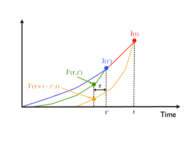
where $\tilde{J^{i}}(\tau,t^{\prime})=\tilde{J}(t^{\prime}-\tau)\Psi(\tau)$. Figure 9 illustrates how the new infection rate at time $t^{\prime}$ depends on the infection rate at time $t^{\prime}-\tau$.

$\tilde{\zeta}(\tau,t^{\prime})$ is the probability function that an infection at time $t^{\prime}$ was caused by any of these individuals. $\tilde{\zeta}(\tau,t^{\prime})$ can be written as

$$\tilde{\zeta}(\tau,t^{\prime})=\frac{\tilde{J^{i}}(\tau,t^{\prime})\tilde{\Theta}(\tau,t^{\prime})}{\int_{0}^{t}\tilde{J^{i}}(\tau^{\prime},t^{\prime})\tilde{\Theta}(\tau^{\prime},t^{\prime})d\tau^{\prime}}.$$ (32)

Figure 9: Dependency of the rate of new infections at time $t^{\prime}$, $\tilde{J}(t^{\prime})$, on the rate of new infections at time $t^{\prime}-\tau$, $\tilde{J}^{i}(\tau,t^{\prime})$. The blue and red curves show the rates of new infections by time $t^{\prime}$ and $t$, respectively. The green and yellow curves show the fraction of those that remained infectious for at least $\tau$ and $\tau+t-t^{\prime}$ units of time, respectively.

Substituting the expressions of $\tilde{\eta}(\tau,t^{\prime},t)$ and $\tilde{\zeta}(\tau,t)$ in Equation (30) we obtain

$$\tilde{I}^{r}(t)+\tilde{R}^{r}(t)=\int_{0}^{t}\tilde{J}(t^{\prime})\left[1-\frac{\int_{0}^{t}\tilde{J^{i}}(\tau+t-t^{\prime},t)\tilde{\Theta}(\tau,t)d\tau}{\int_{0}^{t}\tilde{J}^{i}(\tau,t^{\prime})\tilde{\Theta}(\tau,t)d\tau}\right]dt^{\prime},$$ (33)

Notice that the right-hand side depends only on the rate of new infections, $\tilde{J}(t)$, and disease transmissibility (represented by $\tilde{\Theta}(\tau,t)$). It is also important to notice that outcome of Equation (29) is invariant under $J(t)\longrightarrow{\rm const}*J^{rep}(t)$ where $J^{rep}(t)$ is rate of new reported cases. Finally, we notice that for a disease with the constant removal function, $\lambda_{r}$, $\tilde{J^{i}}(\tau+t-t^{\prime},t)=\tilde{J}(t^{\prime}-\tau)\Psi(\tau)\Psi(t-t^{\prime})$. Therefore, $\tilde{I}^{r}(t)+\tilde{R}^{r}(t)=\tilde{R}(t)$. This means that the first fraction on the right hand side in Equation (27) equals unity, and thus $\tilde{{\mathcal{R}}_{0}^{r}}(t)=\tilde{T}^{r}(t)Z_{x}=1$. The expression for $\tilde{{\mathcal{R}}}_{0}(t)$ then takes the simpler form:

$$\tilde{{\mathcal{R}}}_{0}(t)=\frac{T}{\tilde{T}^{r}(t)}.$$ (34)

An algorithm for the estimation of the basic reproduction number

Using the expressions derived in the previous section, we can compute real time estimates of the basic reproduction number, ${\cal R}_{0}$, assuming some knowledge of the underlying contact network and certaincharacteristics of the disease. For example, if we assume that we know the rate of new infections up to time $t$ ($J(s),$ $s\leq t$), the average excess degree of the underlying contact network, $Z_{x}$, and the removal time density, $\psi(\tau)$, we can calculate an estimator of ${\cal R}_{0}$ as follows.

1. Evaluate the conditional distribution of removal time given that it occurred before time $t$, $\tilde{\psi}^{r}(\tau,t)$, using Equation (24) and $J(t)$.

2. Calculate $\tilde{T}(\tau,t)$ by equating the left- and right-hand side of Equation (27). We should use equation (25) to evaluate the left-hand side of (27). It is worth mentioning that since we use only one equation, we can estimate only one parameter. This means that we must assume a functional form for $\tilde{T}(\tau,t)$ that depends on at most one parameter value. For example, we could assume that $\tilde{T}(\tau,t)={\cal T}(\tau)\tilde{{\cal A}}(t)$, where ${\cal T}(\tau)$ denotes the dependence of the transmissibility on the age of infection and $\tilde{{\cal A}}(t)$ denotes an amplitude effect that captures the stochasticity of the transmissibility as a function of time. Assuming that ${\cal T}(\tau)$ is given, then $\tilde{T}(\tau,t)$ depends only on the multiplicative parameter $\tilde{{\cal A}}(t)$.

3. Calculate an estimator of the expected transmissibility, $\hat{T}(t)$, using $\tilde{T}(\tau,t)$, $\psi(\tau)$ and Equation (3). Notice that the dependence of $\hat{T}(t)$ on $t$ denotes that we are using only information up to time $t$.

4. The estimated reproduction number at time $t$ is given by ${\cal\hat{R}}_{0}(t)=Z_{x}\hat{T}(t)$.

The above algorithm can be modified depending on the information available for the estimation. For example, if there is enough empirical evidence to determine the distribution of the duration of infectiousness as well as the recovery rate of individuals in advance, then the methodology can be used to shed light on the structure of the underlying contact network by estimating $Z_{x}$. Examples of this and other applications of the methodology are given below. But first, a demonstration of the theoretical aspects of our analytical framework. For more details please see [28]

Numerical results

To test the framework presented so far, we performed epidemic spread simulations on the two networks introduced earlier (binomial and exponential) and in each case collected the “time series” of case counts resulting from the simulations.

Constant infectivity and removal functions

In Figure 10 we present the basic reproduction number of the removed individuals, ${\mathcal{R}}_{0}^{r}(t)$, as a function of the number of removed individuals, $R(t)$. The symbols show the results from direct counting during the simulation, whereas the lines show the results obtained from analytically evaluating (after setting $\tilde{T}(\tau,t)=T(\tau)$ and $\tilde{\Theta}(\tau,t)=\frac{dT(\tau)}{d\tau}$ in the left- and right-hand sides of Equation (27)) each of the terms in Equation (27). The green/blue and red/pink colors correspond to the left and right hand side of Equation (27), respectively. The small asymptotic deviation of our estimate for the exponential network comes from finite size effects [29] (for more details, see figure 13 in the appendix).

Figure 10: The estimated basic reproduction number of removed individuals for the binomial (left panel; $z_{1}=5$, $\lambda_{i}=0.12771$ and $\lambda_{r}=0.25$) and exponential (right panel; $\kappa=4$) networks in terms of the number of removed individuals. RHS and LHS represent the right and left hand side of Eq. (27), respectively. The solid curve represents the “analytical” calculation of Eq. (27) and the symbols show the “exact” values of RHS and LHS for this specific realization of the epidemic process.

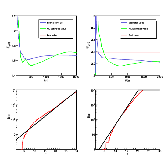
Figure 11 shows our estimated basic reproduction number (blue line) for the binomial (left panel) and exponential (right panel) networks as a function of the number of removed individuals available by time $t$. The“true” values (red line) are ${\mathcal{R}}_{0}=1.6864$ and $2.3749$, respectively. For comparison, the figure also shows the ${\mathcal{R}}_{0}$ estimates obtained from equation Eq. (18), which is equivalent to the Wallinga-Lipsitch (WL) methodology. To compute the WL estimates we require knowledge of the epidemic exponential phase’s growth rate ($\alpha$). For each simulation, we estimated $\alpha$ from the logarithm of the cumulative incidence using simple linear regression and a window of four units of time of data for each time point. The figure shows that in both cases our estimator converges and becomes stable quicker than the WL estimator. This is because our methodology does not make an explicit assumption of exponential epidemic growth and is therefore able to incorporate and appropriately weight the information from the stochastic phase of the epidemic.

Figure 11: Top panels. Estimated basic reproduction number for the binomial (left panel; $z_{1}=5$, $\lambda_{i}=0.12771$ and $\lambda_{r}=0.25$) and exponential (right panel; $\kappa=4$) networks in terms of the number of removed individuals. The red line corresponds to the real value of the basic reproduction number. The blue line shows the estimated ${\mathcal{R}}_{0}$ from our methodology. For comparison, the green line shows the ${\mathcal{R}}_{0}$ estimates obtained from Eq. (18) and estimation of the growth rate during the exponential phase ($\alpha$). Bottom panels. The number of removed individuals by time $t$ (logarithmic scale). The red line shows the number of removed individuals from a realization of the epidemic process. For comparison, the black line shows the theoretical exponential phase of the epidemic process.

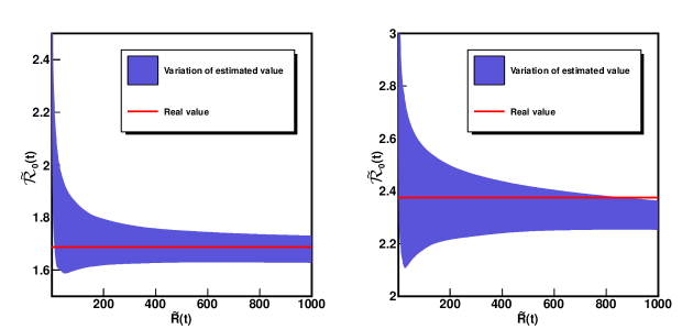
In order to assess the variability of our estimator, we simulated one hundred different realizations of the epidemic process and then estimated the value of ${\mathcal{R}}_{0}$ for each of them. Figure 12 shows the mean estimated value plus/minus one standard deviation (averaging across realizations) for each network. Notice that the variability for the exponential network is bigger than for the binomial network. We attribute this to the fact that the exponential degree distribution has a larger variance. In addition, the ${\mathcal{R}}_{0}$ estimate for the exponential network also appears to have a negative bias. As mentioned above, we attribute this phenomena to finite size effects, which are stronger for this network in comparison to the binomial.

Figure 12: The estimated basic reproduction number for the binomial (left panel; $z_{1}=5$, $\lambda_{i}=0.12771$ and $\lambda_{r}=0.25$) and exponential (right panel; $\kappa=4$) networks in terms of the number of removed individuals. The red line corresponds to the real value of the basic reproduction number. The blue area shows the variation of the estimated value for a hundred different realizations.

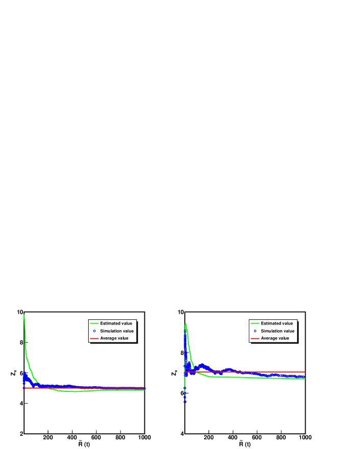
It is worth noting that $\tilde{T}^{r}(t)$ is a function of $\lambda_{i}(\tau)$, $\lambda_{r}(\tau)$ and $J(t)$ (see Equations (3), (24) and (25)). Therefore, when $\lambda_{r}$ is constant, the condition $\tilde{T}^{r}(t)Z_{x}=1$ allows one to evaluate, for a given time series, one of the three quantities $\lambda_{i}$, $\lambda_{r}$ or $Z_{x}$, if the other two quantities are assumed to be known (this statement holds even if $\lambda_{r}$ is a function of time, in which case the more complex Equation (27) should be used). Examples of the estimation of $\lambda_{i}$ or $Z_{x}$ when the other quantities are assumed to be known are shown in the following.

As mentioned earlier $\tilde{T}^{r}(t)$ is a function of $\lambda_{i}(\tau)$, $\lambda_{r}(\tau)$ and $J(t)$ (see Equations (3), (24) and (25)). Therefore, when $\lambda_{r}$ is constant, the condition $\tilde{T}^{r}(t)Z_{x}=1$ allows one to evaluate, for a given time series, one of the three quantities $\lambda_{i}$, $\lambda_{r}$ or $Z_{x}$, if the other two quantities are assumed to be known (this statement holds even if $\lambda_{r}$ is a function of time, in which case the more complex Equation (27) should be used). For instance, we simulated again the epidemic on the binomial and exponential networks presented earlier, but this time with constant values for $\lambda_{r}$ and $\lambda_{i}$. Using these values and the derived/calculated $\tilde{J}(t)$, we calculated the value of $Z_{x}$, which is presented in Figure (13) for the binomial (left panel) and exponential (right panel) networks. The green lines show our estimates using the above condition, while the red lines represent the true values. The blue symbols are the result of the direct count from simulation. It is interesting to note that the excess degree of infected individuals in the simulation very quickly tends to the average value for the binomial network. This explains in part the excellent agreement of our estimate and the true basic reproduction number for the binomial network shown in figure 11. However for the exponential network, the excess degree of infected individuals in the simulation has a higher variability and does not agree as well with the corresponding average excess degree. This is mainly due to finite size effects, which in this case cause an excess degree of infected individuals lower than the average value. And this produces in turn biases in the estimation of ${\mathcal{R}}_{0}$, like those shown in figure 11, and emphasizes the importance of heterogeneity effects for a network such as the exponential. Finally we should mention that all the discrepancies discussed above can be removed, or at least reduced, if one incorporates the true average excess degree from the simulation (blue dots) in Equation (25), instead of a theoretical average excess degree. This could be done if detailed data on the transmission chain and the contacts of infected individuals during an epidemic were available.

Figure 13: Estimates for the value of $Z_{x}$ for the binomial (left) and exponential (right) networks, when $\lambda_{i}$ and $\lambda_{r}$ are known. The red line and green curves correspond to the average and the estimated excess degree.

Time-dependent infectivity and removal functions

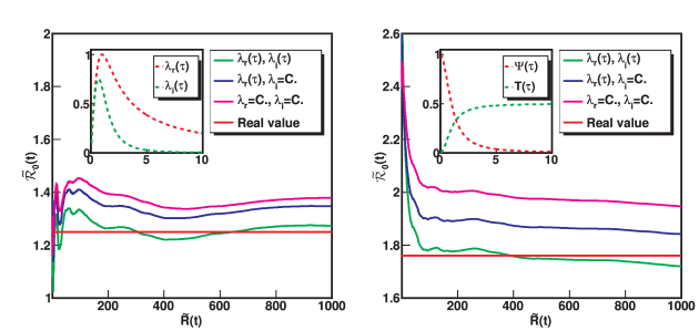
As another example, we use time-dependent infectivity and removal functions to simulate the epidemic process. Specifically, we assume that $\lambda_{i}(\tau)=\tau/(1+\tau^{2})(1+0.5\tau^{2})$ and $\lambda_{r}(\tau)=2\tau/(1+\tau^{2})$. These choices lead to the following expressions for $T(\tau)$ and $\Psi(\tau)$, $T(\tau)=0.5\tau^{2}/(1+\tau^{2})$ and $\Psi(\tau)=1/(1+\tau^{2})$ (or $\psi(\tau)=2\tau/(1+\tau^{2})^{2}$). Figure 14 shows the estimated reproduction number for the binomial (left panel; $z_{1}=5$) and exponential (right panel; $\kappa=4$) networks in terms of the number of removed individuals. The real values in this case are $1.25$ for the binomial and $1.76$ for the exponential network. The true values are shown in red and the estimated values in green. As discussed above, the estimation of the basic reproduction number is performed as follows (assuming that $\lambda_{r}(\tau)$ and $Z_{x}$ are known). 1) For each $t$, we use Equation (27) with $\tilde{T}(\tau,t)=\frac{\tilde{A}(t)\tau}{1+\tau^{2}}$ and $\tilde{\Theta}(\tau,t)=\frac{2\tilde{A}(t)\tau}{(1+\tau^{2})^{2}}$ and then find the $\tilde{A}(t)$ so that the left- and right-hand sides of the equation are equal. 2) We then use the calculated $\tilde{A}(t)$ to obtain the expected transmissibility using Equation (3). Finally we calculate the basic reproduction number, ${\cal R}_{0}=Z_{x}T$. This approach can be used for a specific disease to find the amplitude of the infectivity function, $\tilde{A}(t)$, assuming we know the dependence of $\tilde{\Theta}(\tau,t)$ (or $\tilde{T}(\tau,t)$) on the age of infection, $\tau$. Figure 14 also shows the estimated values of ${\mathcal{R}}_{0}$ that we get if we assume (erroneously) instead that either $\lambda_{i}$ is constant (blue curve) or that both $\lambda_{i}$ and $\lambda_{r}$ are constant (pink curve). The results show that although the methodology is sensitive to misspecifications in the functional forms of $\lambda_{i}$ and $\lambda_{i}$, the estimated ${\mathcal{R}}_{0}$ values are still relatively close to the true value.

Figure 14: The estimated basic reproduction number for the binomial (left panel; $z_{1}=5$, $\lambda_{i}=\tau/(1+\tau^{2})(1+0.5\tau^{2})$ and $\lambda_{r}=2\tau/(1+\tau^{2})$) and exponential (right panel; $\kappa=4$) networks in terms of the number of removed individuals. The red line and green curves correspond to the real and the estimated value. The blue line shows the estimates if we incorrectly assume that $\lambda_{i}$ is constant. The pink line shows the corresponding estimates if we incorrectly assume that both $\lambda_{i}$ and $\lambda_{r}$ are constant

Sensitivity Analysis

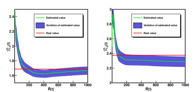
Figure 15 shows the sensitivity of the estimated reproduction number to misspecifications of the excess degree. To test this, we vary the assumed excess degree between $\{4-6\}$ for the binomial network (true value equal to $5$) and between $\{6.04-8.04\}$ for the exponential network (true value equal to $7.04$). The results show that although we assumed a misspecification in the excess degree of up to $20\%$ for the binomial and up to $14.2\%$ for the exponential network, the estimates had an error of at most $3\%$ and $3.1\%$, respectively. As described earlier in the description of the algorithm, we can use Equation (27) to estimate one model parameter, in this case $\lambda_{i}$. And then use its value to evaluate the expected transmissibility and then the expected reproduction number (the first identity in Equation (29)). This shows the usefulness of Equation (27), which acts as a strong constraint that allows us to estimate the basic reproduction number with good precision regardless of misspecification in other input parameters.

Figure 15: The estimated basic reproduction number for the binomial (left panel; $z_{1}=5$, $\lambda_{i}=0.12771$ and $\lambda_{r}=0.25$) and exponential (right panel; $\kappa=4$) networks in terms of the number of removed individuals. The green curve and red line correspond to the estimated (with the correct excess degree) and real value of the basic reproduction number. The blue area shows the variation of the estimated value with respect to change of the excess degree.

Discussion

Using concepts from network theory and stochastic processes, we presented a method that provides a reliable estimate of the basic reproduction number, ${\mathcal{R}}_{0}$. Our method takes into account the stochasticity in disease spread and does not make an explicit assumption about exponential epidemic growth and therefore is able to provide estimates of ${\mathcal{R}}_{0}$ at an early stage of an outbreak (i.e., before the exponential regime). We provided the details of calculations and compared our results at each step against simulations. Case notification data (time series) is the main input to this analytical framework. As an outbreak begins to unfold, the pattern of spread depends substantially on the structure of the underlying contact network. In fact, this dependency manifests itself in the formation of the time series of newly infected cases. The proposed methodology highlights the interplay between the heterogeneity in contacts (network structure), estimates of the basic reproduction number and infection transmissibility. Depending on the circumstances, this methodology can be used to infer other useful quantities as well. For infectious pathogens that cause repeated outbreaks, there is enough empirical evidence to establish the distribution of the duration of infectiousness as well as the recovery rate of individuals. In this case, in addition to the basic reproduction number, the proposed methodology can shed light on the structure of the underlying contact network by estimating the mean excess degree $Z_{x}$. This is an important piece of information, because in many circumstances it is not possible to capture and build a detailed contact network among individuals based on some network generative rules. The importance of this quantity becomes more apparent when an emerging infectious disease strikes a population. In this circumstance, there is much less information on the characteristics of the disease such as the duration of infectiousness and recovery rate, which in turn determine the transmissibility of disease. Knowledge of disease transmissibility during the early stage of an epidemic can play a crucial role, as effective and cost-effective public health intervention strategies hinge on the degree of contagiousness of a disease. On the other hand, before the spread of disease becomes rampant, the structure of the contact network within a population remains more or less stable. Therefore, the estimated value of $Z_{x}$ obtained during epidemic lulls, from the time series corresponding to common infections, can be used to estimate the transmissibility of an emerging infectious disease at the early stage of an outbreak. We demonstrated this concept with two examples. Our estimate for the basic reproduction number converges quickly, thus enabling epidemiologists and policymakers to identify the optimal control strategies, in real time and even before or at the beginning of the exponential growth of an epidemic.

Appendix

Simulation Algorithm

To perform Monte Carlo simulations of an epidemic propagation on a contact network, one first requires explicit knowledge of the network structure. In this article we use the method described in [27, 29] to produce a contact network, given a specific degree distribution. Briefly, (i) sample a random degree sequence ${k_{j}}$ of length $N$ from the degree distribution ${p_{k}}$, (ii) make sure that $\sum_{j}k_{j}$ is an even number since a link is composed of two stubs by reducing the degree of a random individual by one if necessary, (iii) for each $j$, produce a node with $k_{j}$ stubs, (iv) randomly choose a pair of unconnected stubs and connect them together; repeat until all unconnected stubs are exhausted, (v) test for the presence of self-loops and repeated links. Remove the faulty stubs by randomly choosing a pair of connected stubs and rewire them by switching stubs. Repeat until no self-loops and/or repeated links are found.

To simulate the spread of disease on a contact network in continuous time we follow a Tau-Leaping approach [33, 34, 35], which we describe below. The processes of disease transmission along one link and the removal of infectious individuals are controlled by $\lambda_{i}(\tau)$ and $\lambda_{r}(\tau)$, respectively. We divide time into intervals of length $\Delta t$ and ensure that $\lambda_{i}(\tau)\Delta t$ and $\lambda_{r}(\tau)\Delta t$ are small enough, such that the expected epidemic curve does not vary much by reducing $\Delta t$ even further. At every $\Delta t$ step, each infectious individuals recovers with probability $\lambda_{r}(\tau_{j})\Delta t$, where $\tau_{j}$ is the age of infection of individual $j$. If an infectious individual does not recover, then s/he infects independently each of his/her susceptible contacts with probability $\lambda_{i}(\tau_{j})\Delta t$.

Table 1: Notation

Quantity	Symbol	Description
Degree distribution	$p_{k}$	Probability that a randomly chosen vertex has degree $k$.
Average degree	$z_{1}$	Average degree of vertices in a network calculated by $z_{1}=\left\langle k\right\rangle$.
Excess degree	$Z_{x}$	Average degree of a vertix chosen by sampling an edge (calculated by $Z_{x}=\left\langle k^{2}-k\right\rangle$ $\left\langle k\right\rangle$).
Infection hazard or Infectivity function	$\lambda_{i}(\tau)$	Instantaneous rate of infection. $\lambda_{i}(\tau)\delta\tau$ gives the probability of disease transmission across an edge between infection age $\tau$ and $\tau+\delta\tau$, given it occurred after age $\tau$.
Removal hazard or removal function	$\lambda_{r}(\tau)$	Instantaneous removal rate. $\lambda_{r}(\tau)\delta\tau$ gives the removal probability of an infectious individual between its infection age $\tau$ and $\tau+\delta\tau$, given it occurred after age $\tau$.
Transmissibility	$T(\tau)$	Probability of disease transmission by infection age $\tau$. It is calculated by $T(\tau)=1-\exp\left(-\int_{0}^{\tau}\lambda_{i}(\tau^{\prime})d\tau^{\prime}\right)$.
Removal distribution	$1-\Psi(\tau)$	$\Psi(\tau)$ gives the probability of not being removed by age of infection $\tau$. $\Psi(\tau)=\exp\left(-\int_{0}^{\tau}\lambda_{r}(\tau^{\prime})d\tau^{\prime}\right)$.
Removal probability density	$\psi(\tau)$	$\psi(\tau)=-d\Psi(\tau)/d\tau$.
Expected transmissibility	$T$	Probability of disease transmission along one edge, $T=\int_{0}^{\infty}\psi(\tau)T(\tau)d\tau$.
Basic reproduction number	${\cal R}_{0}$	Expected number of infections a typical infected individual can cause in a fully susceptible population, ${\cal R}_{0}=Z_{x}T$.

Table 2: Notation

Quantity	Symbol	Description
Rate of new infections	$\tilde{J}(t)$	$\tilde{J}(t)\delta t$ gives the number of new infections between times $t$ and $t+\delta t$.
	$\tilde{\Theta}(\tau,t)$	Fraction of active S-I edges where disease is actually transmitted exactly at time $t$.
# of infectious individuals	$\tilde{I}(t)$	Total number of infectious individuals at time $t$, $\tilde{I}(t)=\int_{0}^{t}\tilde{J}(t-\tau)\tilde{\Psi}(\tau,t)d\tau$.
# of removed individuals	$\tilde{R}(t)$	Total number of removed individuals at time $t$, $\tilde{R}(t)=\int_{0}^{t}\tilde{J}(t-\tau)[1-\tilde{\Psi}(\tau,t)]d\tau$.
	$\tilde{R}^{r}(t)$	Total number of removed individuals at time $t$ whose predecessor is already removed.
	$\tilde{R}^{i}(t)$	Total number of removed individuals at time $t$ whose predecessor is still infectious.
	$\tilde{I}^{r}(t)$	Total number of infectious individuals at time $t$ whose predecessor is already removed.
	$\tilde{I}^{i}(t)$	Total number of infectious individuals at time $t$ whose predecessor is still infectious.
	$\tilde{{\cal Z}}_{x}^{r}(t)$	Total number of excess links of removed individuals, calculated by Eq. (22).
Transmissibility of removed individuals	$T^{r}(t)$	Gives the transmissibility of removed individuals at time $t$ and it is calculated by Eqs. (23) and (25).
	$\chi(\tau)$	$\chi(\tau)\delta\tau$ gives the expected number of new infections produced by an infectious individual between ages of infection $\tau$ and $\tau+d\tau$.
Generation interval distribution	$\hat{\chi}(\tau)$	$\hat{\chi}(\tau)\delta\tau$ gives the conditional probability that given an infection, it occurred between ages of infection $\tau$ and $\tau+d\tau$.

References

- 1. R. M. Anderson and R. M. May, Infectious diseases of humans (Oxford: Oxford University Press, 1991).
- 2. H. Anderson and T. Britton, Stochastic Epidemic Models and their Statistical Analysis (Springer: Berlin, 2000).
- 3. K. Dietz, Stat. Math. Res. 2, 23 (1993).
- 4. W. O. Kermack and A. G. McKendrick, Proc. Roy. Soc. Lond. A 115, 700 (1927).
- 5. J. Ma and D. J. D. Earn, Bulletin of Math. Biol. 68, 679 (2006).
- 6. J. Arino, F. Brauer, P. van den Driessche, J. Watmough, and J. Wu, Math. Biosci. Eng. 4, 159 (2007).
- 7. F. Brauer, Math. Biosci. Eng. 5, 681 (2008).
- 8. H. W. Hethcote, SIAM Rev. 42, 599 (2000).
- 9. M. Lipsitch et al., Science 300, 1966 (2003).
- 10. C. Fraser et al., Science 324, 1557 (2009).
- 11. H. Abbey, Human. Biol. 24, 201 (1952).
- 12. N. T. J. Bailey, The mathematical theory of infectious diseases and its applications, Second ed. (Hafner Press [Macmillan Publishing Co., Inc.] New York, 1975).
- 13. C. L. Addy, I. M. Longini, and M. Haber, Biometric 47, 961 (1991).
- 14. F. Ball, Adv. Appl. Prob. 18, 289 (1986).
- 15. N. Becker, Biometric 32, 769 (1976).
- 16. F. Ball and P. Donnelly, Stoch. Process. Appl. 55, 1 (1995).
- 17. P. Guttorp, Statistical Inference for Branching Processes (Wiley: New York, 1991).
- 18. J. Wallinga and P. Teunis, Am. Jour. Epid. 160, 509 (2004).
- 19. S. Cauchemez et al., Emerging Infect Dis 12, 110 (2006).
- 20. S. Cauchemez, P. Y. Boelle, G. Thomas, and A. J. Valleron, Am. Jour. Epid. 164, 591 (2006).
- 21. L. F. White and M. Pagano, Stat. Med. 27, 2999 (2008).
- 22. H. Nishiura Biomed. Eng. Online, 10, 15 (2011).
- 23. K. G. Katrie1, R. Yaari, A. Huppert U. Roll and L. Stone Jour. of the Roy. Soc. Inter., 8, 85 (2011).
- 24. D. Balcan, H. Hu, B. Goncalves, P. Bajardi, C. Poletto, J. J. Ramasco, D. Paolotti, N. Perra, M. Tizzoni, W. V. Broeck, V. Colizza and A. Vespignani BMC Med., 7, 45, (2009).
- 25. H. Nishiura1, G. Chowell, M. Safan and C. Castillo-Chavez Theo. Bio. and Med. Model., 7, 1 (2010).
- 26. J. Wallinga and M. Lipsitch, Proc. Biol. Sci. 274, 599 (2007).
- 27. M. E. J. Newman, Phys. Rev. E 66, 016128 (2002).
- 28. B. Pourbohloul, A. Ahued, B. Davoudi, R. Meza, L. A. Meyers, D. M. Skowronski, I. Villaseñor, F. Galván, P. Cravioto, D. J. D. Earn, J. Dushoff, D. Fisman, W. J. Edmunds, N. Hupert, S. V. Scarpino, J. Trujillo, M. Lutzow, J. Morales, A. Contreras, C. Chávez, D. M. Patrick and R. C. Brunham , et al. Infl. and other Respi. Viruses, 3, 215 (2009).
- 29. P. A. Noel, B. Davoudi, L. J. Dube, R. C. Brunham, and B. Pourbohloul, Phys. Rev. E 79, 026101 (2009).
- 30. D. R. Cox and D. Oakes, Analysis of survival data (Chapman & Hall, 1984).
- 31. A. J. Lotka, Ann. of Math. Stat. 10, 1 (1939).
- 32. M. Kot, Elements of Mathematical Ecology (Cambridge University Pres, 2002).
- 33. T. G. Daniel, The Jour. of Chem. Phys. 115, 1716 (2001).
- 34. T. G. Daniel and R. P. Linda, The Jour. of Chem. Phys. 119, 8229 (2003).
- 35. D. J. Higham, SIAM Rev. 50, 347 (2008).