sFit: a method for background subtraction in maximum likelihood fit

Yuehong Xie University of Edinburgh, Edinburgh EH9 3JZ, United Kingdom

Abstract
This paper presents a statistical method to subtract background in maximum likelihood fit, without relying on any separate sideband or simulation for background modeling. The method, called sFit, is an extension to the sPlot technique originally developed to reconstruct true distribution for each date component. The sWeights defined for the sPlot technique allow to construct a modified likelihood function using only the signal probability density function and events in the signal region. Contribution of background events in the signal region to the likelihood function cancels out on a statistical basis. Maximizing this likelihood function leads to unbiased estimates of the fit parameters in the signal probability density function.

1 Introduction

The method of maximum likelihood is a common procedure used for parameter estimation in analysis of experimental data. Suppose the probability density function (pdf) $P(x;\theta)$ with unknown parameters $\theta$ describes a set of $N$ independent measurements $x_{e}$. The values of $\theta$ that maximize the likelihood function

$$L(\theta)=\prod_{e=1}^{N}P(x_{e};\theta)$$ (1)

are taken to be the estimators for $\theta$. The conventional method to include background in maximum likelihood fit requires to write the total pdf as

$$P(x;\theta,f_{s})=f_{s}P_{s}(x;\theta)+(1-f_{s})P_{b}(x)$$ (2)

where $f_{s}$ is the fraction of signal events in th data sample, $P_{s}(x;\theta)$ and $P_{b}(x)$ are the signal and background pdf respectively. Usually the background pdf $P_{b}(x)$ needs to be obtained from either Monte Carlo simulation or separate sidebands. The latter requires to divide data into signal region and sidebands using discriminating variables $y$ which are supposed to be uncorrelated with $x$ for the background component. Some problems may arise with this method: $P_{b}(x)$ may be too complicated to parameterize; the parameterization of $P_{b}(x)$ obtained from simulation may be unreliable; the sidebands may have very different $P_{b}(x)$ distributions from the signal region if they are too far away from the signal region; the sidebands may contain a significant signal component if they are too close to the signal region. Therefore, it is highly desirable to have an alternative method which does not rely on background parameterization from either simulation or separate sidebands. This paper provides a solution by generalizing the sPlot technique [1], originally developed to reconstruct true distribution of $x$ for the signal component using sWeights defined as functions of $y$, into a modified maximum likelihood method, called sFit.

2 The sFit method

Suppose $x$ are uncorrelated with the discriminating variables $y$, i.e. the distribution of $x$ is independent of $y$, for both signal and background components. The data sample contains $N_{s}$ signal events and $N_{b}$ background events. The distributions of $y$ for signal and background are denoted as $F_{s}(y)$ and $F_{b}(y)$ respectively. We assume that $N_{s}$, $N_{b}$, $F_{s}(y)$ and $F_{b}(y)$ are known. Following the formalism of the sPlot technique, we define a sWeight function for the signal component:

$$W_{s}(y)={V_{ss}F_{s}(y)+V_{sb}F_{b}(y)\over N_{s}F_{s}(y)+N_{b}F_{b}(y)},$$ (3)

where the matrix $V$ is obtained by inverting the matrix

$$V_{ij}^{-1}=\sum_{e=1}^{N}{F_{i}(y_{e})F_{j}(y_{e})\over(N_{s}F_{s}(y_{e})+N_{b}F_{b}(y_{e}))^{2}}.$$ (4)

The sWeight for each event, $W_{s}(y_{e})$, can be calculated. The basic idea of the sPlot technique is that the histogram of $x_{e}$ weighted by $W_{s}(y_{e})$ represents the true distribution of $x$ for the signal component, because the background contribution to the histogram cancels out due to this choice of $W_{s}(y_{e})$.

We can extend this idea one step further and define a weighted likelihood function

$$L_{W}(\theta)=\prod_{e=1}^{N}[P_{s}(x_{e};\theta)]^{W_{s}(y_{e})}.$$ (5)

We expect that background contribution to this likelihood function $L_{W}(\theta)$ cancels on a statistical basis, therefore $\theta$ can be estimated by maximizing $L_{W}(\theta)$.

3 Application

We apply the sFit method in a simple case in time-dependent analysis of B decays. The signal pdf of proper time $t$ is

$$P_{s}(t;A,\Gamma)=C_{1}e^{-\Gamma t}(1+A\sin(\Delta mt))$$ (6)

where $C_{1}$ is a normalization factor, $\Delta m=17$ ${\rm ps}^{-1}$ is known, $A$ and $\Gamma$ are parameters to be determined. Dependence of the pdf on initial flavour of the B meson is not considered for simplicity. The background events have a different time distribution

$$P_{b}(t;\Gamma_{b})=C_{2}e^{-\Gamma_{b}t},$$ (7)

where $C_{2}$ is a normalization factor, and $\Gamma_{b}$ is unknown. The discriminating variable is the B mass. The signal events have a known gaussian mass distribution with a standard deviation $\sigma_{m}=15$ ${\rm MeV}$ and mean $m_{0}=5369$ ${\rm MeV}$. The background events have a known flat distribution. The signal mass window is chosen to be centered at $m_{0}$. We consider scenarios with different half mass window size $S_{m}$ and different number of signal and background events in the signal mass window.

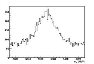
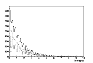
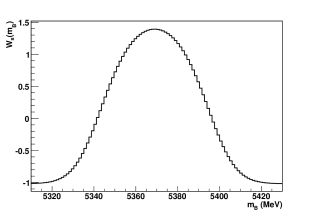
As an example, Figure 1 shows the distribution of the B mass $m_{B}$, the total time distribution, as well as the signal and background time distributions reconstructed using the sWeights, for the scenario $S_{m}/\sigma_{m}=6$, $N_{s}=5000$ and $N_{b}/N_{s}=1.5$. The $W_{s}(m_{B})$ function for this scenario is shown in Figure 2. The fact that $W_{s}(m_{B})$ has positive values in the high signal purity region around $m_{0}$ and negative values in the low purity area illustrates why the background contribution cancels in both the sPlot and the sFit methods.

Figure 1: Distributions from a data set with $S_{m}/\sigma_{m}=6$, $N_{s}=5000$ and $N_{b}/N_{s}=1.5$. Left: the B mass distribution; right: the total time distribution (solid), as well as the signal time distribution (dashed) and background time distribution (dot-dashed) reconstructed using the sPlot technique.

Figure 2: $W_{s}$ as a function of the B mass $m_{B}$ for the scenario $S_{m}/\sigma_{m}=6$, $N_{s}=5000$ and $N_{b}/N_{s}=1.5$.

500 toy data sets are generated for each scenario with

$$A=0.5,\,\Gamma=0.65\,{\rm ps}^{-1},\,\Gamma_{b}=0.8\,{\rm ps}^{-1}.$$ (8)

We perform fit to each data set using two different methods: the sFit method described in Section 2 and a conventional maximum likelihood method for reference based on Equation 1 and the total pdf

$$P(t;A,\Gamma,\Gamma_{b})=f_{s}P_{s}(t;A,\Gamma)F_{s}(m)+(1-f_{s})P_{b}(t;\Gamma_{b})F_{b}(m)$$ (9)

where the shape of the background pdf $P_{b}(t;\Gamma_{b})$ is assumed to be known except the parameter $\Gamma_{b}$.

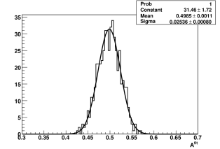
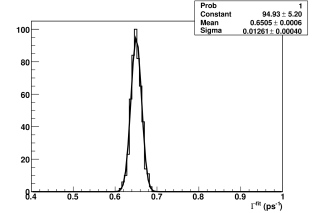
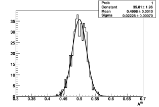
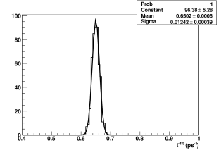
For each scenario and each fit method, the statistical errors and mean values of the parameter $A$ and $\Gamma$ are obtained using a single gaussian fit to their estimated values from the 500 data sets. An example is shown in Figure 3 and Figure 4 for the scenario $S_{m}/\sigma_{m}=6$, $N_{s}=5000$ and $N_{b}/N_{s}=1.5$. The results for different scenarios are summarized in the Table 1 and Table 2 for the sFit method and reference method respectively.

It can be seen that the sFit method gives unbiased estimates of the fit parameters $A$ and $\Gamma$. The statistical errors of the parameter estimates obtained with the sFit method are bigger than the errors of the estimates obtained with the reference methods. This has two reasons: while the background contribution to $L_{W}$ cancels, part of the signal contribution is also lost due to the negative sWeights in the low purity area, and the size of the loss depends on the size of the signal mass window; the cancellation of background contribution is not exact due to statistical fluctuation, and the size of the fluctuation depends on the background level in the signal region. In general, the larger the signal mass window, the smaller the precision difference between the two methods; the lower the background level, the smaller the precision difference between the two methods. We should keep in mind that the reference method takes full advantage of the knowledge of the background time distribution, which is usually unavailable or unreliable in real data analysis, therefore the parameter errors in Table 2 are too optimistic and should be regarded as lower limits rather than realistic estimates. The sWeight function defined in Equation 3 is not the unique way to define event weight function in order to can cancel the background contribution to the weighted likelihood function. It would be interesting to investigate if the sWeight is the optimal choice of event weight function that minimizes the parameter errors.

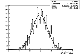
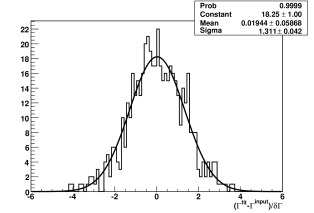
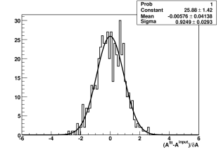
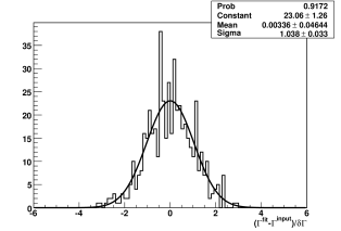
Figure 5 and Figure 6 show the distributions of $(A^{fit}-A^{input})/\delta A$ and $(\Gamma^{fit}-\Gamma^{input})/\delta\Gamma$ for the sFit method and reference method respectively, where $\delta A$ and $\delta\Gamma$ are the parameter errors estimated by the Minuit program according to $\ln L=\ln L_{max}-{1\over 2}$. Apparently the errors obtained this way using the weighted likelihood function $L_{W}$ are underestimated, because the effect of background fluctuation is not properly accounted for. Reliable error estimates can be obtained from Monte Carlo simulation.

Figure 3: Distributions of the estimated values of $A$ (left) and $\Gamma$ (right) obtained with the sFit method, with superimposed gaussian fits, for the scenario $S_{m}/\sigma_{m}=6$, $N_{s}=5000$ and $N_{b}/N_{s}=1.5$. The input values are $A=0.5$ and $\Gamma=0.65\,{\rm ps^{-1}}$.

Figure 4: Distributions of the estimated values of $A$ (left) and $\Gamma$ (right) obtained with the reference method, with superimposed gaussian fits, for the scenario $S_{m}/\sigma_{m}=6$, $N_{s}=5000$ and $N_{b}/N_{s}=1.5$. The input values are $A=0.5$ and $\Gamma=0.65\,{\rm ps^{-1}}$.

$S_{m}/\sigma_{m}$, $N_{s}$, $N_{b}/N_{s}$	$\sigma(A)$	mean of $A$	$\sigma(\Gamma)$ (${\rm ps}^{-1}$)	mean of $\Gamma$ (${\rm ps}^{-1}$)
4, 5000, 1	0.0304	0.502	0.0134	0.6504
6, 5000, 1.5	0.0254	0.498	0.0126	0.6504
4, 5000, 0.5	0.0243	0.501	0.0115	0.6511
6, 5000, 0.75	0.0223	0.501	0.0107	0.6496

Table 1: Statistical errors and mean values of $A$ and $\Gamma$ from 500 fits using the sFit method for different scenarios. Errors of the numbers are on the last digits. The input values are $A=0.5$ and $\Gamma=0.65\,{\rm ps^{-1}}$.

$S_{m}/\sigma_{m}$, $N_{s}$, $N_{b}/N_{s}$	$\sigma(A)$	mean of $A$	$\sigma(\Gamma)$ (${\rm ps}^{-1}$)	mean of $\Gamma$ (${\rm ps}^{-1}$)
4, 5000, 1	0.0251	0.502	0.0129	0.6506
6, 5000, 1.5	0.0223	0.500	0.0124	0.6502
4, 5000, 0.5	0.0215	0.500	0.0113	0.6511
6, 5000, 0.75	0.0211	0.501	0.0105	0.6496

Table 2: Statistical errors and mean values of $A$ and $\Gamma$ from 500 fits using the conventional maximum likelihood method for different scenarios. Errors of the numbers are on the last digits. The input values are $A=0.5$ and $\Gamma=0.65\,{\rm ps^{-1}}$.

Figure 5: Distributions of $(A^{fit}-A^{input})/\delta A$ (left) and $(\Gamma^{fit}-\Gamma^{input})/\delta\Gamma$ (right) obtained with the sFit method, with superimposed gaussian fits, for the scenario $S_{m}/\sigma_{m}=6$, $N_{s}=5000$ and $N_{b}/N_{s}=1.5$.

Figure 6: Distributions of $(A^{fit}-A^{input})/\delta A$ (left) and $(\Gamma^{fit}-\Gamma^{input})/\delta\Gamma$ (right) obtained with the sFit method, with superimposed gaussian fits, for the scenario $S_{m}/\sigma_{m}=6$, $N_{s}=5000$ and $N_{b}/N_{s}=1.5$.

4 Conclusions

The sFit method presented in this paper fully exploits the idea of background cancellation for maximum likelihood fit. If the variables $x$ are uncorrelated with the discriminating variables $y$ for both signal and background components, one can define an event weight function of $y$ which can be used not only to reconstruct the signal distribution of $x$, but also for parameter estimation from the distributions of $x$ in maximum likelihood fit without explicitly modeling the background. The likelihood function constructed using the event weights and the signal pdf of $x$ is free from background contribution on a statistical basis. Maximizing the likelihood function leads to unbiased parameter estimates. This method can largely reduce systematic uncertainties due to unreliable background model obtained from either sidebands or simulation at a cost of modest increases in the statistical errors.

References

- [1] M. Pivk and F. R. Le Diberder, Nucl. Instrum. Meth. A555, 356 (2005), physics/0402083.