Quantum dynamics of cavity assisted photoassociation of Bose-Einstein condensed atoms

Abstract

We explore the quantum dynamics of photoassociation of Bose-Einstein condensed atoms into molecules using an optical cavity field. Inside of an optical resonator, photoassociation of quantum degenerate atoms involves the interaction of three coupled quantum fields for the atoms, molecules, and the photons. The feedback created by a high-Q optical cavity causes the cavity field to become a dynamical quantity whose behavior is linked in a nonlinear manner to the atoms inside and where vacuum fluctuations have a more important role than in free space. We develop and compare several methods for calculating the dynamics of the atom-molecule conversion process with a coherently driven cavity field. We first introduce an alternate operator representation for the Hamiltonian from which we derive an improved form of mean field theory and an approximate solution of the Heisenberg-Langevin (HL) equations that properly accounts for quantum noise in the cavity field. It is shown that our improved mean field theory corrects several deficiencies in traditional mean field theory based on expectation values of annihilation/creation operators. Also, we show by direct comparison to numerical solutions of the density matrix equations that our approximate quantum solution of HL equations gives an accurate description of weakly or undriven cavities where mean field theories break down.

I Introduction

In the last decade, there has been considerable interest in creating ultra-cold quantum degenerate molecular systems because of the potential for improved understanding of molecular physics and interactions, exploring new types of many-body systems such as condensates of dipolar molecules and the BCS-BEC crossover, and the generation of entangled atoms by controlled dissociation of molecules search-progress-optics . Two techniques, magnetically tunable Feshbach resonances and photoassociation, have been developed to create ultra-cold molecules that start first from laser cooled atoms and then induce controlled chemical bonding between the atoms. Feshbach resonances are the most widely used and have been successfully applied by numerous research groups to create molecular dimers starting from either a Bose-Einstein condensate (BEC) mol-1 ; durr ; xu-2003 ; herbig or a Fermi gas regal-2003 ; strecker-2003 ; jochim-2003 ; cubizolles-2003 . This work culminated in the formation of a molecular Bose-Einstein condensate (MBEC) mol-BEC-K ; mol-BEC-Li .

Besides Feshbach resonances, experiments have demonstrated that two-photon Raman photoassociation can also be used to create ultra-cold molecules wynar ; julienne1 ; rom ; winkler . Two-photon photoassociation has the added benefit that the frequency difference between the two optical fields can be used to select a particular rotational-vibrational state including the rotational-vibrational ground statetsai ; jones . This gives photoassociation an advantage over Feshbach resonances since Feshbach molecules are often very weakly bound in high energy vibrational states that quickly decay to lower lying vibrational states via inelastic collisions xu-2003 ; yurovsky ; mukaiyama . Recent work has has used two-photon Raman transitions to create rovibrational ground state molecules from weakly bound Feshbach molecules ni-2008 ; lang-2008 .

Here we address the problem of two-photon Raman photoassociation of an atomic BEC inside of an optical cavity that is coherently driven. Due to the cavity, photons circulate and interact with the atoms and molecules many times before finally exiting in a manner analogous to a feedback loop. This feedback amplifies the back action of the atoms and molecules onto the cavity field causing the light to now become a dynamical part of the process. In our particular case, we assume that one of the optical fields used to induce the atom-molecule conversion is a quantized mode of a driven Fabrey-Perot resonator while the other field does not correspond to a cavity mode but is rather a laser directed transverse to the cavity with sufficient intensity to be treated as a ’classical’ undepleted pump. Our model therefore involves the interaction of four particles: two atoms are ’destroyed’ and a molecule and cavity photon are ’created’ and vice versa. Consequently, the atom-molecule-cavity photon interaction is analogous to $\chi^{(3)}$ susceptibility in nonlinear optics. This is different from molecule formation via a Feshbach resonance or free space photoassociation with undepleted classical lasers where the conversion only involves two quantum fields: atoms and molecules and is the matter-wave analog of second harmonic generation of photons with a $\chi^{(2)}$ susceptibility. Coherent photoassociation inside of a cavity therefore offers the prospect of novel nonlinear dynamics between the atomic, molecular, and cavity fields and the possibility of enhanced control over the atom-molecule conversion process.

In an earlier work we analyzed the mean field dynamics and steady state behavior of cavity assisted photoassociation markku while here we extend that work to study the role of quantum fluctuations on the dynamics. We analyze the quantum dynamics for the atomic, molecular, and cavity fields by several methods. First, an alternate operator representation for the Hamiltonian is introduced that has an algebra analogous to angular momentum. These new operators allow us to derive from the Heisenberg-Langevin equations both an improved form of mean field theory and an approximate solution for the quantum dynamics that treats the atom-molecule populations classically but the cavity field and atom-molecule-photon coherences fully quantum mechanically. The improved mean field theory incorporates quantum correlations between the atom and molecules. It also includes a contribution due to vacuum fluctuations of the atomic and molecular fields that corrects a deficiency in traditional mean field theory, which fails to predict atom-molecule Rabi oscillations for resonant transitions because the solution approaches and becomes stuck at an unstable equilibrium point. We also compare the improved mean field theory with our approximate quantum solution and direct integration of the density matrix equations in the case of small photon and atom numbers. It is shown that our approximate quantum solution provides a more accurate description in the case that the cavity driving is weak or absent in comparison to mean field theories since in this case the dynamics are initiated by the vacuum fluctuations of the cavity field.

Before proceeding we note that only a few papers have previously considered photoassociation inside of a cavity olsen1 ; olsen2 . However, unlike our model, theirs was based on single photon photoassociation, which is impractical for observing coherent atom-molecule dynamics because the molecules created are in electronic excited states and can rapidly decay due to spontaneous emission. The authors of Ref. olsen1 ; olsen2 employed the positive-P distributionQuantumNoise to analyze the quantum dynamics of the three coupled fields. The positive-P distribution has a tendency to become numerically unstable for long times in highly nonlinear quantum optical systems as the stochastic trajectories begin to sample unphysical regions of phase space and must be stabilized by proper choice of a stochastic gauge, which is often difficult to properly determine drummond . In fact, it has been shown that the equations presented in the earlier work olsen1 ; olsen2 are numerically stable only for a limited range of parameters and that the photon blockade effect predicted in that work does not in general occurjaeyoon-thesis .

The paper is organized as follows: In section II, we present our model for cavity assisted photoassociation and the density matrix equations of motion. Additional details for the physical model can be found in Ref. markku . In section III, we derive our improved mean field theory and an approximate solution of the Heisenberg-Langevin equations for the dynamics based on a pseudo-angular momentum operator representation. In section IV, we compare numerical results for the density matrix, approximate Heisenberg-Langevin equations, and mean field theories.

II Model

Our starting point is a BEC of atoms inside of an optical cavity, as depicted in Fig. 1. The atoms as well as the molecules formed from them can be trapped inside of the cavity using a far-off resonant optical trap similar to what has been recently demonstrated with single atoms in a cavity boca . At temperatures $T\approx 0$, we can assume that all of the atoms are in the ground state of the trapping potential with wave function $\psi_{a}(r)$. Additionally, the atoms are assumed to have all been prepared in the same hyperfine state denoted by $|a\rangle$. Pairs of atoms in $|a\rangle$ are coupled to electronically excited molecular states $|I_{\nu}\rangle$, where $\nu$ denotes the vibrational state of the molecule, via a pump laser with Rabi frequency $\Omega_{l}$ and frequency $\omega_{l}$. The pump is treated as a large amplitude undepleted source and therefore changes in $\Omega_{l}$ due to absorption or stimulated emission are neglected.

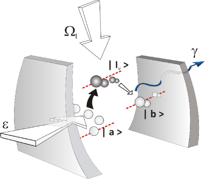
Figure 1: (Color online) Schematic diagram showing the system under consideration. The kets $|a\rangle$, $|b\rangle$, and $|I_{\nu}\rangle$ denote pairs of atoms, electronic ground state molecules, and electronically excited molecules, respectively. $\varepsilon$ is the rate at which the cavity is coherently driven by an external laser while $\gamma$ is the decay rate for photons in the cavity. $\Omega_{l}$ is the pump laser that drives the $|a\rangle\rightarrow|I_{\nu}\rangle$ transition.

The excited molecular states are coupled to molecules in their electronic and vibrational ground state, $|b\rangle$, via a single cavity mode. The ground state wave function for the center of mass of the molecules is denoted by $\psi_{b}(x)$. Emission of a photon into the cavity mode takes a molecule from an excited state to its electronic ground state. Coupling to a single mode can be achieved by insuring that only a single cavity mode is close to two-photon resonance for the atom-molecule Raman transition and by positioning the atoms and molecules around an antinode of the cavity field. The discrete mode structure of the cavity allows one to select a particular vibrational state in the electronic ground-state manifold of the molecules provided the cavity line width, $\gamma$, is less than the vibrational level spacing, which can be as high as $1$GHz tsai . This would imply a cavity Q-factor of $Q\gg 10^{6}$, which has already been achieved with individual atoms trapped inside of a Fabrey-Perot resonatorboca . The cavity field frequency is $\omega_{c}$ and the vacuum Rabi frequency for the $|I_{\nu}\rangle\rightarrow|b\rangle$ transition is $g_{cav}$.

The internal energies of states $|I_{\nu}\rangle$ and $|b\rangle$ relative to pairs of atoms in $|a\rangle$ are $\omega_{\nu}$ and $\Delta\omega<0$, respectively. We assume that the detuning between the excited states and the pump and cavity fields satisfy, $\Delta_{\nu}=\omega_{\nu}-\omega_{l}\approx(\omega_{\nu}-\Delta\omega)-\omega_{c}\gg|g_{cav}|,|\Omega_{l}|,\gamma_{\nu}$ where $\gamma_{\nu}^{-1}$ is the lifetime of $|I_{\nu}\rangle$ due to spontaneous emission. Under these conditions the excited states can be adiabatically eliminated, leading to two-photon Raman transitions between $|a\rangle$ and $|b\rangle$ with the resulting Hamiltonian for the atom-cavity-molecule system,

$$\hat{H}_{am}=\hbar\delta\hat{b}^{\dagger}\hat{b}+i\frac{\hbar g}{2}(\hat{a}^{\dagger 2}\hat{b}\hat{e}-\hat{a}^{2}\hat{b}^{\dagger}\hat{e}^{\dagger})+\hbar\chi_{a}\hat{a}^{\dagger 2}\hat{a}^{2}+\hbar\chi_{b}\hat{b}^{\dagger 2}\hat{b}^{2}.$$ (1)

Here $\hat{a}$, $\hat{b}$, and $\hat{e}$ are bosonic annihilation operators for atoms, ground state molecules, and cavity photons, respectively. Moreover, the molecular and photon operators have been written in a rotating frame, $\hat{b}\rightarrow\hat{b}\exp[+i(\omega_{c}-\omega_{l})t]$ and $\hat{e}\rightarrow\hat{e}\exp[-i\omega_{c}t]$, to remove all time dependence from the interaction term. The two-photon detuning is defined as $\delta=(\Delta\omega-(\omega_{l}-\omega_{c}))$.

The terms proportional to $\chi_{a}$ and $\chi_{b}$ represent the two body interactions between pairs of atoms and pairs of molecules, respectively. Interactions involving an atom interacting with a molecule can be written as $\chi_{ab}\hat{N}_{a}\hat{N}_{b}=\frac{1}{4}\chi_{ab}\left(\hat{N}^{2}-\hat{N}_{a}^{2}-4\hat{N}_{b}^{2}\right)$ where $\hat{N}=\hat{N}_{a}+2\hat{N}_{b}$ is the total number operator and $\hat{N}_{a}=\hat{a}^{\dagger}\hat{a}$ and $\hat{N}_{b}=\hat{b}^{\dagger}\hat{b}$. Since the total number of particles is conserved, $[\hat{H}_{am},\hat{N}]=0$, $\chi_{ab}$ can be absorbed into a redefinition of $\chi_{a}$ and $\chi_{b}$.

The dynamics of the cavity are described by two competing processes. The first process is cavity decay, which can be treated using the standard Born-Markov master equation for the density operator QuantumNoise ,

$$\frac{d\rho}{dt}|_{damping}=\frac{\gamma}{2}\left(2\hat{e}\rho\hat{e}^{\dagger}-\hat{e}^{\dagger}\hat{e}\rho-\rho\hat{e}^{\dagger}\hat{e}\right)$$ (2)

In addition to this, the cavity is coherently driven by an external laser described by the following Hamiltonian,

$$H_{pump}=i\hbar(\varepsilon\hat{e}^{\dagger}-\varepsilon^{*}\hat{e}).$$ (3)

where we have assumed that the driving laser is resonant with the cavity mode. The complete equation of motion for the density operator is then given by,

$$\frac{d\rho}{dt}=\frac{1}{i\hbar}[H_{pump}+H_{am},\rho]+\frac{\gamma}{2}\left(2\hat{e}\rho\hat{e}^{\dagger}-\hat{e}^{\dagger}\hat{e}\rho-\rho\hat{e}^{\dagger}\hat{e}\right).$$ (4)

The two-photon Rabi frequency is $g=-i\int d^{3}x\psi_{b}^{*}(x)[g_{cav}u(x)\Omega_{l}^{*}(x)\sum_{\nu}I^{*}_{a,\nu}I_{b,\nu}/\Delta_{\nu}]\psi_{a}(x)$. $I_{\ell,\nu}$ are the Frank-Condon factors for the $|\ell=a,b\rangle\rightarrow|I_{\nu}\rangle$ transitions drummond-STIRAP and since typically $|\Omega_{l}|/|\Delta_{\nu}|$ and $I_{a,\nu}\ll 1$, $g/\gamma\ll 1$ even if the cavity is in the strong coupling regime $|g_{cav}|>\gamma$

We represent the density operator in the basis of eigenstates of $\hat{N}_{a}$, and $\hat{N}_{e}=\hat{e}^{\dagger}\hat{e}$, $|n_{a},n_{e}\rangle$. Because $n_{a}+2n_{b}=N$ is a constant of motion, the molecule number, $n_{b}$, is completely determined by $n_{a}$. The density matrix in this basis, $\langle n^{\prime}_{a},n^{\prime}_{e}|\rho|n_{a},n_{e}\rangle$, is then unwrapped into a column vector, $\vec{\rho}$, so that Eq. 4 can be written as a matrix equation, $d\vec{\rho}/dt=\bf{M}\vec{\rho}$, which can now be integrated using a first order Euler method savage-1990 ,

$$\vec{\rho}(t)=\lim_{k\rightarrow\infty}\left(I+(t/k)\bf{M}\right)^{k}\vec{\rho}(0)$$ (5)

This method has the advantage of using less memory than higher order ODE solvers but is still limited to small numbers of atoms and photons. In the next section we develop approximate equations of motion that incorporate quantum effects but can deal with much larger experimentally realistic numbers of atoms ($\sim 10^{3}-10^{6}$) and photons.

III Pseudo-Angular Momentum Description

Here we develop a representation of the model developed in the previous section using pseudo-angular momentum operators that simplify the form of the Hamiltonian and use this representation to derive Heisenberg-Langevin equations for the system. We then obtain mean field equations and approximate equations for the quantum dynamics from the Heisenberg-Langevin equations.

For an initial state that is an eigenstate of $\hat{N}=\hat{N}_{a}+2\hat{N}_{b}$, the solution of Eq. 4 will at all later times continue to be an eigenstate of $\hat{N}$ with the same eigenvalue $N$. In this case, we can introduce new operators vardi-anglin

$$\hat{L}_{x} = \hat{L}_{+}+\hat{L}_{-}=\frac{\sqrt{2}\left(\hat{a}^{\dagger}\hat{a}^{\dagger}\hat{b}+\hat{b}^{\dagger}\hat{a}\hat{a}\right)}{N^{3/2}}$$ (6)

$$\hat{L}_{y} = -i(\hat{L}_{+}-\hat{L}_{-})=\frac{\sqrt{2}\left(\hat{a}^{\dagger}\hat{a}^{\dagger}\hat{b}-\hat{b}^{\dagger}\hat{a}\hat{a}\right)}{iN^{3/2}}$$ (7)

$$\hat{L}_{z} = \frac{2\hat{b}^{\dagger}\hat{b}-\hat{a}^{\dagger}\hat{a}}{N}$$ (8)

and $\hat{L}_{+}^{\dagger}=\hat{L}_{-}$. These operators have the following commutation relations,

$$\left[\hat{L}_{\pm},\hat{L}_{z}\right] = \pm\frac{4}{N}\hat{L}_{\pm}$$ (9)

$$\left[\hat{L}_{+},\hat{L}_{-}\right] = \frac{3}{2N}\left(\hat{L}_{z}-1\right)\left(\hat{L}_{z}+1/3\right)-\frac{2}{N^{2}}$$ (10)

The commutation relations $\left[\hat{L}_{\pm},\hat{L}_{z}\right]$ are of the same form as for angular momentum but the equivalence to angular momentum is ruined by the commutator $\left[\hat{L}_{+},\hat{L}_{-}\right]$. We therefore refer to them as pseudo-angular momentum operators.

Equation 1 can be rewritten in terms of these new operators as

$$\hat{H}_{am}=\frac{\hbar}{4}N\bar{\delta}\hat{L}_{z}+\frac{\hbar}{4}N^{2}\bar{\chi}\hat{L}_{z}^{2}+i\hbar g\left(\frac{N}{2}\right)^{3/2}\left(\hat{L}_{+}\hat{e}-\hat{L}_{-}\hat{e}^{\dagger}\right)$$ (11)

where $\bar{\chi}=\chi_{a}+\chi_{b}/4$ and $\bar{\delta}=\delta+N(-2\chi_{a}(1-1/N)+(\chi_{b}/2)(1-2/N))$.

It is well known that Born-Markov density matrix equations such as Eq. 4 are fully equivalent to Heisenberg-Langevin equations with Markov noise operators in the Heisenberg picture QuantumNoise , which in this case have the form

$$\frac{d}{dt}\hat{L}_{-} = i\bar{\delta}\hat{L}_{-}+iN\bar{\chi}\left(\hat{L}_{z}\hat{L}_{-}+\hat{L}_{-}\hat{L}_{z}\right)+g(2N)^{-1/2}\hat{e}$$ (12)

$$- g\left(\frac{3}{4}\right)\left(\frac{N}{2}\right)^{1/2}\left(\hat{L}_{z}-1\right)\left(\hat{L}_{z}+1/3\right)\hat{e}$$

$$\frac{d}{dt}\hat{L}_{z} = -g(2N)^{1/2}\left(\hat{L}_{+}\hat{e}+\hat{L}_{-}\hat{e}^{\dagger}\right)$$ (13)

$$\frac{d}{dt}\hat{e} = \varepsilon-\frac{\gamma}{2}\hat{e}-g\left(\frac{N}{2}\right)^{3/2}\hat{L}_{-}+\hat{F}(t)$$ (14)

Here $\hat{F}(t)$ is a Markov noise operator for the fluctuations of the electromagnetic reservoir coupled to the cavity mode via the mirrors with zero mean $\langle\hat{F}(t)\rangle=0$ and the two-time correlations $\langle\hat{F}(t)\hat{F}(t^{\prime})\rangle=\langle\hat{F}^{\dagger}(t)\hat{F}(t^{\prime})\rangle=0$ and $\langle\hat{F}(t)\hat{F}^{\dagger}(t^{\prime})\rangle=\gamma\delta(t-t^{\prime})$.

Because the Heisenberg-Langevin are nonlinear operator equations, they cannot be solved exactly. The simplest approximation is that of mean field theory, which replaces all operators with their c-number expectation values and factorizes products of operators, $\hat{L}_{+}\hat{e}\rightarrow\langle\hat{L}_{+}\rangle\langle\hat{e}\rangle$ thereby ignoring higher order correlations and non-commutativity of operators. This yields three nonlinear c-number differential equations,

$$\frac{d}{dt}L_{-} = i\bar{\delta}L_{-}+i2N\bar{\chi}L_{z}L_{-}+g(2N)^{-1/2}e$$ (15)

$$- g\left(\frac{3}{4}\right)\left(\frac{N}{2}\right)^{1/2}\left(L_{z}-1\right)\left(L_{z}+1/3\right)e$$

$$\frac{d}{dt}L_{z} = -g(2N)^{1/2}\left(L_{+}e+L_{-}e^{*}\right)$$ (16)

$$\frac{d}{dt}e = \varepsilon-\frac{\gamma}{2}e-g\left(\frac{N}{2}\right)^{3/2}L_{-}$$ (17)

where the lack of a hat denotes a c-number expectation value, $A=\langle\hat{A}\rangle$. These equations are unaffected by quantum noise since $\langle\hat{F}(t)\rangle=0$ and according to mean field theory, $\langle\hat{e}\hat{e}^{\dagger}\rangle=\langle\hat{e}^{\dagger}\hat{e}\rangle=e^{*}e$.

We note that this form of the mean field approximation is different from the traditional manifestation with Bose-Einstein condensates or light where annihilation/creation operators for the fields are replaced with c-number expectation values. This form was used in our previous work markku and yielded the equations

$$\dot{a}=-2i\chi_{a}a^{*}a^{2}+ga^{*}be$$ (18)

$$\dot{b}=-i\delta b-2i\chi_{b}b^{2}b^{*}-\frac{g}{2}a^{2}e^{*}$$ (19)

$$\dot{e}=\varepsilon-\frac{\gamma}{2}e-\frac{g}{2}a^{2}b^{*}$$ (20)

where $a=\langle\hat{a}\rangle$, $b=\langle\hat{b}\rangle$, and again $e=\langle\hat{e}\rangle$. In the case that $e(t)$ is treated as a time independent constant, Eqs. 18 and 19 are equivalent to earlier mean field studies of atom-molecule dynamics with Feshbach resonances or photoassociation drummond-STIRAP ; goral ; olsen1 ; search-progress-optics ; gr-jin . By contrast Eqs. 15-17, which we refer to as pseudo-angular momentum mean field theory (PAMMF), represent a higher order approximation for the atomic and molecular fields than Eqs. 18-20, which we refer to as amplitude mean field (AMF) theory. The PAMMF equations automatically incorporate lowest order quantum correlations between the atomic and molecular field operators as a consequence of the pseudo-angular momentum representation, $L_{z}=\langle 2\hat{b}^{\dagger}\hat{b}-\hat{a}^{\dagger}\hat{a}\rangle/N$ and $L_{-}=\sqrt{2}\langle\hat{b}^{\dagger}\hat{a}\hat{a}\rangle/N^{3/2}$. Additionally, Eq. 15 includes the vacuum fluctuations of the matter fields resulting from the last term in the commutator $[\hat{L}_{+},\hat{L}_{-}]$. In the next section we consider the different predictions for the dynamics made by PAMMF and AMF.

Mean field theory typically works well for large amplitude quantum fields. However, initially the cavity field is in the vacuum state and therefore it cannot be used to describe the initial short time behavior $\sim\gamma^{-1}$. Additionally, when the cavity is not driven $\varepsilon=0$, mean field theory completely fails to describe the dynamics, which are initiated by vacuum fluctuations of the cavity field. Therefore we develop a solution to Eqs. 12-14 that properly includes photon noise.

We note that equations 12 and 14 can be linearized and solved exactly if one replaces $\hat{L}_{z}$ with a c-number, $L_{z}$. In the case that the c-number is time independent, this approach would be equivalent to the undepleted pump approximation in nonlinear quantum optics and the Bogoliubov method for weakly interacting BEC’s. We adopt an approach where the c-number $L_{z}$ is instead treated as a dynamical variable whose value is given by the expectation value of Eq. 13. First we express the equations for $\hat{L}_{-}$ and $\hat{e}$ as

$$\frac{d}{dt}\vec{X}=\mathbf{M}\vec{X}+\vec{S}$$ (21)

where $\vec{X}^{T}=\left(\hat{L}_{-},\hat{e}\right)$ and $\vec{S}^{T}=\left(0,\varepsilon+\hat{F}(t)\right)$ while

$$\mathbf{M}(t)=\left(\begin{array}[]{cc}i\Delta\Omega(t)&-g\beta(t)\\ -g(N/2)^{3/2}&-\gamma/2\\ \end{array}\right)$$ (22)

and $\Delta\Omega=\bar{\delta}+2N\bar{\chi}L_{z}(t)$ and $\beta(t)=(3/4)(N/2)^{1/2}(L_{z}(t)^{2}-2L_{z}(t)/3-1/3)-1/\sqrt{2N}$. The correlation matrix,

$$\mathbf{C}(t)=\langle\vec{X}(t)\vec{X}(t)^{\dagger}\rangle=\left(\begin{array}[]{cc}\langle\hat{L}_{-}\hat{L}_{+}\rangle&\langle\hat{L}_{-}\hat{e}^{\dagger}\rangle\\ \langle\hat{e}\hat{L}_{+}\rangle&\langle\hat{e}\hat{e}^{\dagger}\rangle\\ \end{array}\right)$$ (23)

gives us information about the number of cavity photons and the coherence between the cavity field and the atom-molecule fields, which can be used to calculate $L_{z}(t)$. $\mathbf{C}(t)$ has the equation of motion obtained directly from Eq. 21,

$$\frac{d}{dt}\mathbf{C}=\mathbf{M}\mathbf{C}+\mathbf{C}\mathbf{M}^{\dagger}+\left(\begin{array}[]{cc}0&\varepsilon^{*}\langle\hat{L}_{-}\rangle\\ \varepsilon\langle\hat{L}_{-}\rangle^{*}&\gamma+\varepsilon\langle\hat{e}\rangle^{*}+\varepsilon^{*}\langle\hat{e}\rangle\\ \end{array}\right)$$ (24)

Equation 24 forms a closed set along with the equations for the expectation value of Eq. 21 and the expectation value of $\hat{L}_{z}(t)$,

$$\frac{d}{dt}L_{z}=-g(2N)^{1/2}\left(\langle\hat{e}\hat{L}_{+}\rangle+\langle\hat{L}_{-}\hat{e}^{\dagger}\rangle\right)$$ (25)

We refer to this approach that incorporates the quantum noise of the cavity field and atom-molecule-photon coherences while treating the atom-molecule populations classically as the quantum self-consistent population (QSCP) method. In general this QSCP method is valid for large $N\gg 1$ in the same manner as the Bogoliubov theory of weakly interacting condensates search-progress-optics . From the c-number substitution $\hat{L}_{z}\rightarrow L_{z}(t)$, one can see then that the commutation relations Eqs. 9 and 10 are only preserved in the limit $N\rightarrow\infty$. In comparison to AMF and PAMMF equations, Eqs. 24 and 25 properly account for quantum noise of the cavity field. The quantum noise of the photons arise from two sources in the equations for $\mathbf{C}(t)$: $\langle\hat{e}\hat{e}^{\dagger}\rangle=\langle\hat{e}^{\dagger}\hat{e}\rangle+1$ representing the vacuum fluctuations of the cavity mode and the reservoir noise $\langle\hat{F}(t)\hat{F}^{\dagger}(t^{\prime})\rangle=\gamma\delta(t-t^{\prime})$, which appears as $\gamma$ in the equation for $\langle\hat{e}\hat{e}^{\dagger}\rangle$.

IV Numerical Results

In this section we analyze numerical solutions of the AMF, PAMMF, QSCP, and exact density matrix equations. In all simulations we use the initial conditions $N_{a}(0)=N$ atoms, $N_{b}(0)=0$ molecules, and no photons, $N_{e}(0)=0$.

IV.1 Semiclassical Limit, $N\gg 1$ and $\varepsilon\gg\gamma$

When the cavity mode is strongly driven, $\varepsilon\gg\gamma$, the photon noise is negligible and atom-molecule transitions are dominated by stimulated absorption and emission instead spontaneous emission into the cavity mode implying that one should be able to treat the cavity mode classically. Here we compare traditional mean field theory given by AMF with the improved PAMMF mean field theory along with the the QSCP method that incorporates cavity noise.

Figure 2 shows that the PAMMF mean field dynamics (Eqs. 15-17) reproduce qualitatively the behavior of the the QSCP method (Eqs. 24 and 25), which consist of damped Rabi oscillations that approach the final steady state $N_{b}=N/2$ molecules and $N_{e}\approx 0$ photons. For resonant atom-molecule conversion ($\delta=\chi_{a}=\chi_{b}=0$), PAMMF and QSCP agree very closely for the first few Rabi oscillations while for longer times the QSCP solutions oscillate at a slightly higher frequency. For off-resonant transitions ($\delta\neq 0$ or $\chi_{a},\chi_{b}\neq 0$), the agreement becomes increasingly better and they are indistinguishable for $|\delta|\gg g\sqrt{N}$. This indicates that quantum correlations between the cavity field and atom-molecule medium given by $\langle\hat{e}\hat{L}_{+}\rangle$ play a non-negligible role in modifying the dynamics when full molecule conversion can occur.

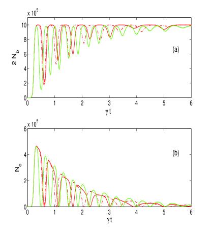
Figure 2: (Color Online) (a) Molecule number and (b) intracavity photon number calculated using the PAMMF mean field equations (solid lines) and QSCP equations (dash dot lines) as a function of time $t$ (in units of $\gamma^{-1}$). In all cases $N=10^{6}$, $g/\gamma=5\times 10^{-5}$, and $\varepsilon/\gamma=100$. Here red lines are for $\delta=\chi_{a}=\chi_{b}=0$ while green lines are for $\delta/\gamma=1$, and $\chi_{a}=\chi_{b}=0$. Note that in the later case (green lines), the two solutions are indistinguishable.

By contrast, the AMF solutions (Eqs. 18-20) exhibit qualitatively very different dynamics from PAMMF and QSCP method in the resonant case as seen in Fig. 3. In the case $\delta=\chi_{a}=\chi_{b}=0$, AMF equations display no Rabi oscillations and instead the molecule number grows monotonically until it reaches the steady state $N_{b}=N/2$. Atom-molecule oscillations are absent because as soon as the atomic condensate is fully depleted, $a(t)=0$, the nonlinear Rabi frequency in Eqs. 18 and 19 vanishes leading to $\dot{b}=0$ and $\dot{a}=0$. This behavior is the same as earlier mean field studies of atom-molecule conversion via Feshbach resonances or photo-association with undepleted lasers goral ; vardi-anglin ; gr-jin . In that case the analytic solution for the molecule number was shown to be $N_{b}(t)=(N/2)\tanh^{2}(\sqrt{2N}|\Omega|t)$ goral where $\Omega$ is atom-molecule coupling, which can be taken to be equivalent to a time independent $g\langle\hat{e}\rangle/2$ in our model.

The AMF solution $N_{b}=N/2$ is an unstable equilibrium vardi-anglin and fluctuations of the atom or molecular fields would excite the system out of this state leading to atom-molecule oscillations. The PAMMF equations incorporate the vacuum fluctuations of the atomic-molecular fields in the term $g(2N)^{-1/2}e$ in Eq. 15. Because of this term, even for $\delta=\chi_{a}=\chi_{b}=0$ when there is full conversion into molecules ($L_{z}(t)=+1$), one still has $\dot{L}_{-}=g(2N)^{-1/2}e$. Figure 4 shows that when $g(2N)^{-1/2}e$ is eliminated from Eq. 15, PAMMF and AMF equations produce virtually identical results comment .

Besides the molecule number, the AMF makes different predictions for the photon number than PAMMF and QSCP. For $\delta=\chi_{a}=\chi_{b}=0$, the PAMMF and QSCP results indicate that the photon number approaches the steady state $N_{e}=0$ while the AMF solution predicts that the photon number grows like $N_{e}=(2\varepsilon/\gamma)^{2}$ as shown in Fig. 5. This behavior is again attributable to the atom-molecule quantum fluctuations. When the AMF solution reaches the unstable equilibrium, $N_{b}=N/2$, the equation for the cavity field reduces to that of an empty cavity, $\dot{e}=\varepsilon-\gamma e/2$. By contrast, the PAMMF mean field equations have the steady state solution $L_{z}=+1$, $e=0$, and $L_{-}=(\varepsilon/g)(2/N)^{-3/2}$ for the resonant case.

For nonzero values of $\delta$, $\chi_{a}$, or $\chi_{b}$, the AMF equations do exhibit oscillations between atoms and molecules since the atom-molecule transition is detuned from perfect resonance, which prevents full conversion into molecules from occurring. For example, for small $|\delta|$, PAMMF show higher frequency larger amplitude oscillations but as $|\delta|$ is increased, the agreement between AMF and PAMMF becomes increasingly better until the solutions are again indistinguishable for $|\delta|\gg g\sqrt{N}$ as seen in Fig. 3.

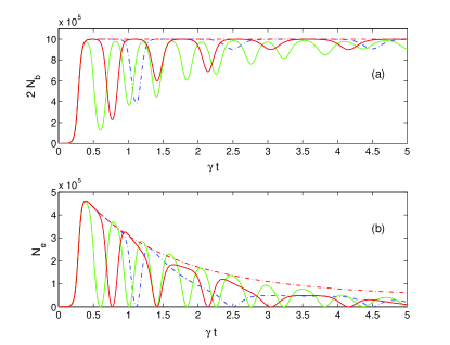
Figure 3: (Color Online) (a) Molecule number and (b) intracavity photon numbers calculated using the PAMMF equations (solid lines) and AMF equations (dash dot lines) as a function of time $t$ (in units of $\gamma^{-1}$). In all cases $N=10^{6}$, $g/\gamma=4\times 10^{-5}$, and $\varepsilon/\gamma=100$. Here red lines are $\delta=\chi_{a}=\chi_{b}=0$; blue lines are $\delta/\gamma=0.0001$ and $\chi_{a}=\chi_{b}=0$; green lines are $\delta/\gamma=1$ and $\chi_{a}=\chi_{b}=0$. Note that in the final case (green lines), PAMMF and AMF are indistinguishable. Also, PAMMF for $\delta/\gamma=0.0001$ (blue solid line) and PAMMF for $\delta=0$ (red solid line) are indistinguishable.

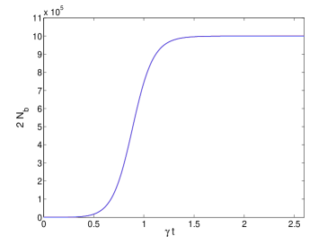
Figure 4: (Color Online) Molecule number calculated using the PAMMF equations without the term $g(2N)^{-1/2}e$ in Eq. 15 (red solid line) and AMF equations (blue solid line). Here $N=10^{6}$, $g/\gamma=10^{-5}$, $\varepsilon/\gamma=100$, $\delta=\chi_{a}=\chi_{b}=0$. The two solutions are indistinguishable.

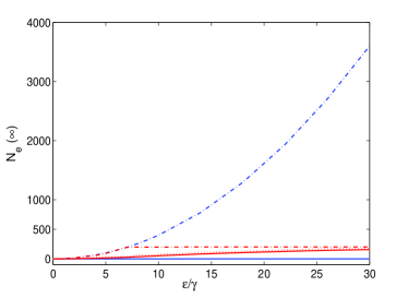
Figure 5: (Color Online) Steady state photon number as a function of $\varepsilon/\gamma$ calculated using the QSCP equations (solid lines), PAMMF equations (dotted lines), and AMF equations (dashed dot lines). Here $N=10^{6}$ and $g/\gamma=5\times 10^{-5}$. Blue lines are for $\delta=\chi_{a}=\chi_{b}=0$ and red lines are $\delta/\gamma=1$ and $\chi_{a}=\chi_{b}=0$.

These results indicate that for off-resonant atom-molecule conversion, all three methods agree. For resonant transitions, the PAMMF and QSCP show atom-molecule Rabi oscillations due to the inclusion of the matter field vacuum fluctuations while the QSCP additionally includes atom-molecule-photon correlations that modify the effective Rabi frequency.

IV.2 Weakly Driven Cavity, $\varepsilon\ll\gamma$

For weak driving, $\varepsilon\ll\gamma$, reservoir noise and cavity vacuum fluctuations are both much stronger than the coherent driving. In this case, AMF and PAMMF equations are expected to give an inaccurate description. In fact, for the limiting case $\varepsilon=0$, both mean field theories predict no dynamics at all since in the absence of photon fluctuations there is nothing to initiate the atom-molecule conversion.

First we show a comparison of the PAMMF and QSCP equations for $N\gg 1$ and $\varepsilon\ll\gamma$ in Fig. 6. As one can see for the QSCP, the conversion of atoms into molecules starts much earlier. This is easily understood if one solves the QSCP equations for $L_{z}(t)$ using perturbation theory. Solving for $L_{z}(t)$ for short times from the initial condition $L_{z}(0)=-1$, one finds that

$$L_{z}(t)\approx-1+(tg\sqrt{N})^{2}(1-1/N)(1-\gamma t/6),$$ (26)

which is correct to order $t^{3}$ even for arbitrary $\varepsilon$. The cavity driving $\varepsilon$ only contributes to $L_{z}(t)$ at order $t^{4}$ in perturbation theory with the term

$$L_{z}(t)|_{\varepsilon}=(g\sqrt{N})^{2}(1-1/N)|\varepsilon|^{2}t^{4}/4.$$ (27)

From which we see that the cavity fluctuations dominate the short time behavior and it is only for later times that the atoms feel the affect of the cavity driving.

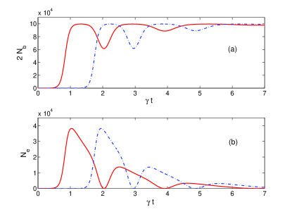
Figure 6: (Color Online) (a) Molecule number and (b) intracavity photon numbers calculated using the PAMMF equations (blue dash dot lines) and QSCP equations (red solid lines) as a function of time $t\gamma$ for the parameters $N=10^{5}$, $g/\gamma=1.5\times 10^{-4}$, $\delta=\chi_{a}=\chi_{b}=0$ and $\varepsilon/\gamma=0.01$.

In Figs. 7 and 8 we show solutions of the density matrix (Eq. 5), QSCP, and PAMMF solutions for initial atom numbers $N_{a}=64$ and $\varepsilon=0$ and $0.1\gamma$. One can see that for times long enough for nearly full conversion to occur, the QSCP and density matrix solutions show very good agreement while the PAMMF either predicts no dynamics ($\varepsilon=0$) or dynamics that start significantly later ($\varepsilon=0.1\gamma$). The molecule number, $N_{b}$, for both the PAMMF and QSCP solution approach a steady value that is below that of the density matrix, $N_{b}=N/2$. This is a consequence of the c-number approximation for $\hat{L}_{z}$, which is only valid for $N\gg 1$. Our simulations indicate that this error vanishes as $N\rightarrow\infty$ and both PAMMF and QSCP indicate full molecule conversion on resonance. Unfortunately, our solutions of Eq. 5 are limited to a maximum of 64 atoms and photons.

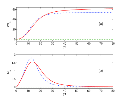
Figure 7: (Color Online) (a) Molecule number and (b) intracavity photon numbers calculated using the density matrix (Eq. 5) (red solid lines), PAMMF equations (green dashed lines), and QSCP equations (blue dashed dot lines) as a function of time $t\gamma$ for the parameters $N=64$, $g/\gamma=0.01$, $\delta=\chi_{a}=\chi_{b}=0$ and $\varepsilon/\gamma=0$.

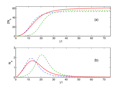
Figure 8: (Color Online) (a) Molecule number and (b) intracavity photon numbers calculated using the density matrix (Eq. 5) (red solid lines), PAMMF equations (green dashed lines), and QSCP equations (blue dashed dot lines) as a function of time $t\gamma$ for the parameters $N=64$, $g/\gamma=0.01$, $\delta=\chi_{a}=\chi_{b}=0$ and $\varepsilon/\gamma=0.1$.

V Conclusions

Here we have compared several different approaches for analyzing the dynamics of intracavity photoassociation. It has been shown that traditional mean field theory, which replaces annihilation/creation operators with c-numbers, fails to provide an accurate description of the dynamics since it ignores the quantum fluctuations of both the matter fields and the cavity field. We developed two new approaches that go beyond traditional mean field theory by introducing a different operator representation for the Hamiltonian similar to angular momentum. When mean field theory is applied to the new operator representation, the resulting equations properly incorporate vacuum fluctuations of the matter fields, which are necessary for atom-molecule Rabi oscillations to occur. The second approach, QSCP, which goes one step further by also incorporating quantum fluctuations and reservoir noise of the cavity field, provides an accurate description of the short time behavior that agrees with exact numerical solutions of the density matrix equations. This final method that incorporates photon noise works even when the cavity in not driven, which is when both mean field theories completely fail. Even more important, the QSCP equations can be easily solved numerically for arbitrary numbers of atoms and photons while the density matrix can only be solved for relatively small numbers of atoms and photons, typically less than a 100 each.

In a future work we plan to improve upon the QSCP method in a manner that will allow us calculate both squeezing and number fluctuations of the fields.

The work was supported by the National Science Foundation award no. 0757933.

References

- (1) C. P. Search and P. Meystre, Nonlinear and quantum optics of atomic and molecular fields, in Progress in Optics, Vol. 47, p. 139-214, edited by E. Wolf (Elsevier, Amsterdam, 2005).
- (2) E. A. Donley, N. R. Claussen, S. T. Thompson, and C. E. Wieman, Nature (London) 417, 529 (2002).
- (3) S. Durr, T. Volz, A. Marte, and G. Rempe, Phys. Rev. Lett. 92, 020406 (2004).
- (4) K. Xu, T. Mukaiyama, J. R. Abo-Shaeer, J. K. Chin, D. E. Miller, and W. Ketterle, Phys. Rev. Lett. 91, 210402 (2003).
- (5) Jens Herbig, Tobias Kraemer, Michael Mark, Tino Weber, Cheng Chin, Hanns-Christoph Nägerl, Rudolf Grimm, Science 301, 1510 (2003).
- (6) C. A. Regal, C. Ticknor, J. L. Bohn, and D. S. Jin, Nature (London) 424, 47 (2003)
- (7) K. E. Strecker, G. B. Partridge, and R. G. Hulet, Phys. Rev. Lett. 91, 080406 (2003).
- (8) S. Jochim et al., Phys. Rev. Lett. 91, 240402 (2003).
- (9) J. Cubizolles et al., Phys. Rev. Lett. 91, 240401 (2003).
- (10) M. Greiner, C. A. Regal, and D. S. Jin, Nature (London) 426, 537 (2003).
- (11) M. W. Zwierlein, C. A. Stan, C. H. Schunck, S. M. F. Raupach, S. Gupta, Z. Hadzibabic, W. Ketterle, Phys. Rev. Lett. 91, 250401 (2003); S. Jochim, M. Bartenstein, A. Altmeyer, G. Hendl, S. Riedl, C. Chin, J. Hecker Denschlag, Science 302, 2101 (2003).
- (12) R. Wynar R.S. Freeland, D.J. Han, C. Ryu, D.J. Heinzen, Science 287, 1016 (2000);
- (13) P. S. Julienne, K. Burnett, Y. B. Band, and W. C. Stwalley, Phys. Rev. A 58, R797 (1998); D. Heinzen, R. Wynar, P. Drummond, and K. Kheruntsyan, Phys. Rev. Lett. 84, 5029 (2000).
- (14) Tim Rom, Thorsten Best, Mandel, Artur Widera, Markus Greiner, Theodor W. Hänsch, and Immanuel Bloch, Phys. Rev. Lett. 93, 073002 (2004).
- (15) K. Winkler, G. Thalhammer, M. Theis, H. Ritsch, R. Grimm, and J. Hecker Denschlag, Phys. Rev. Lett. 95, 063202 (2005).
- (16) C. C. Tsai R. S. Freeland, J. M. Vogels, H. M. J. M. Boesten, B. J. Verhaar, and D. J. Heinzen, Phys. Rev. Lett. 79, 1245 (1997).
- (17) Kevin M. Jones, Eite Tiesinga, Paul D. Lett, and Paul S. Julienne, Rev. Mod. Phys. 78, 483 (2006).
- (18) V. A. Yurovsky, A. Ben-Reuven, P. S. Julienne, and C. J. Williams, Phys. Rev. A 60, R765 (1999); V. A. Yurovsky and A. Ben-Reuven, Phys. Rev. A 72, 053618 (2005).
- (19) T. Mukaiyama, J. R. Abo-Shaeer, K. Xu, J. K. Chin, and W. Ketterle, Phys. Rev. Lett. 92, 180402 (2004).
- (20) K. K. Ni, S. Ospelkaus, M. H. G. de Miranda, A. Pe’er, B. Neyenhuis, J. J. Zirbel, S. Kotochigova, P. S. Julienne, D. S. Jin, and J. Ye, Science 322, 231 (2008).
- (21) F. Lang, K. Winkler, C. Strauss, R. Grimm, and J. Hecker Denschlag, Phys. Rev. Lett. 101, 133005 (2008).
- (22) Markku Jaaskelainen, Jaeyoon Jeong, and Christopher P. Search, Phys. Rev. A 76, 063615 (2007).
- (23) M. K. Olsen, J. J. Hope, and L. I. Plimak, Phys. Rev. A 64, 013601 (2001).
- (24) M. K. Olsen, L. I. Plimak, and M. J. Collett, Phys. Rev. A 64, 063601 (2001).
- (25) C. W. Gardiner and P. Zoller, ”Quantum Noise: A Handbook of Markovian and Non-Markovian Quantum Stochastic Methods with Applications to Quantum Optics” (Springer-Verlag, Berlin, 2004).
- (26) M. R. Dowling, M. J. Davis, P. D. Drummond, and J. F. Corney, J. Comp. Phys. 220, 549 (2007); P. Deuar and P. D. Drummond, J. Phys. A 39, 2723 (2006).
- (27) Jaeyoon Jeong, Ph.D. thesis, Stevens Institute of Technology, 2007.
- (28) A. Boca, R. Miller, K. M. Birnbaum, A. D. Boozer, J. McKeever, and H. J. Kimble, Phys. Rev. Lett. 93, 233603 (2004).
- (29) P. D. Drummond and K. V. Kheruntsyan, D. J. Heinzen and R. H. Wynar, Phys. Rev. A 65, 063619 (2002).
- (30) C. M. Savage, Journal of Modern Optics 37, 1711 (1990).
- (31) A. Vardi, V. A. Yurovsky, and J. R. Anglin, Phys. Rev. A 64, 063611 (2001).
- (32) Krzysztof Goral, Mariusz Gajda, and Kazimierz Rzazewski, Phys. Rev. Lett. 86, 1397 (2001).
- (33) Guang-Ri Jin, Chul Koo Kim, and Kyun Nahm, Phys. Rev. A 72, 045602 (2005).
- (34) The authors of Ref. 31 also used the same pseudo-angular momentum representation for their model of atom-molecule conversion via a feshbach resonance/photoassociation but they eliminated the vacuum fluctuation term from their equations arguing that since it scaled like , it was unimportant for . As a result, their solutions didn’t display atom-molecule Rabi oscillations.