Unconventional metallic conduction in two-dimensional Hubbard-Wigner lattices

Abstract

The interplay between long-range and local Coulomb repulsion in strongly interacting electron systems is explored through a two-dimensional Hubbard-Wigner model. An unconventional metallic state is found in which collective low-energy excitations characteristic of the Wigner crystal induce a flow of electrical current despite the absence of one-electron spectral weight at the Fermi surface. Photoemission experiments on certain quarter-filled layered molecular crystals should observe a gap in the excitation spectrum whereas optical spectroscopy should find a finite Drude weight indicating metallic behavior.

I Introduction

Coulomb interactions in two dimensions (2D) can lead to different forms of electron localization ranging from Mott insulatorsImada1 to Wigner crystals Wigner . Half-filled narrow-band systems such as cuprate Bonn ; Lee and organic superconductors Ishiguro ; McKenzie1 display insulating states in their phase diagrams which are not described by band theory approaches. This is due to the strong local Coulomb repulsion driving the system to a Mott metal-insulator transition (MIT) which localizes electrons at each site of the lattice. On the other hand, a gas of electrons in a positive uniform background can localize through Wigner crystallization when the long-range Coulomb repulsion overcomes the kinetic energy, which is relevant to the MIT observed in two-dimensional electron gases (2DEG) at sufficiently low densities Kravchenko ; Abrahams . Besides, there are many 2D crystals with non-integer filled narrow bands which are neither Mott nor Wigner insulators but rather display ”Wigner crystallization on an underlying lattice” (WL) Hubbard78 , with both aspects of electron localization. The family of quarter-filled layered organic materials, $\theta$-(BEDT-TTF)₂MM’(SCN)₄ (M=Rb, Cs, Tl,M’=Zn, Co) represent clean realizations of WL displaying a subtle competition between charge ordering, superconductivity and unconventional metallic phases in their phase diagram Seo . These systems pose the challenging question of whether the interplay between short (Mott) and long-range Coulomb interactions (Wigner) Camjayi08 ; Pankov on a lattice can lead to new ground states and excitations and whether such novel states of matter can be experimentally tested.

Extensions of the Hubbard model including the long-range Coulomb interaction have mostly been limited to one-dimensional Wigner lattices Hubbard78 ; Valenzuela03 ; Fratini04 ; Horsch06 ; Daghofer07 . In these systems the degeneracy of the classical ground state at non-integer fillings leads, in the strongly interacting regime, to low-energy excitations consisting of domain walls with fractional charge. This type of collective excitations, which play a major role in the melting of the Wigner lattice on the one-dimensional chain Fratini04 ; Horsch06 , have been much less explored in two dimensions. Tsiper ; Pollmann Here we find that collective excitations in 2D can give rise to metallic conduction in a charge ordered metallic state (COM) even though there is a finite charge gap in the one-electron spectrum. By combining conductivity and photoemission/tunneling experiments, such an anomalous metallic phase could be clearly identified and discerned from a more conventional charge density wave (CDW) metal, in which the conducting behaviour is ensured by portions of the Fermi surface that remain gapless.

The paper is organized as follows. The model and the numerical method that we use are presented in Sec. II. The main results are contained in Sec. III, and their possible relevance to experimental systems is discussed in Sec. IV. In the appendices we introduce an analytical model valid in the limit of strong long-range Coulomb interactions, that provides a clear interpretation of the numerical results in terms of defects of the checkerboard ordering.

II Model and method

The minimal model to describe the effect of the long-range part of the Coulomb interaction in 2D is the Hubbard-Wigner model (HWM) at one-quarter filling on a square lattice:

$$H=-t\sum_{<ij>\sigma}(c^{\dagger}_{i\sigma}c_{j\sigma}+c^{\dagger}_{j\sigma}c_{i\sigma})+U\sum_{i}n_{i\uparrow}n_{i\downarrow}+\sum_{ij}V_{ij}n_{i}n_{j},$$ (1)

where $c^{\dagger}_{i\sigma}$ creates an electron with spin $\sigma$ on site $i$, the kinetic energy is parametrized by the hopping amplitude $t$ between neighboring sites and the onsite Coulomb interaction by $U$. The long-range contribution is: $V_{ij}=V/|i-j|$, with $|i-j|$ the distance between two different sites on the lattice and $V$ a parameter controlling the strength of the non-local Coulomb repulsion. The model is solved using Lanczos diagonalization on finite clusters of up to $L=18$ sites with periodic boundary conditions. The Coulomb potential between two different sites inside the cluster is calculated from Ewald summations which account for an infinite periodic array of simulation cells. In order to single out the effects introduced by the long-range part of the interaction we compare results of the full model with the extended Hubbard model (EHM) containing $U$ and a nearest-neighbor $V$ only. We deliberately choose a large $U=100t$ in order to disentangle the relevant low-energy excitations of the system, focusing primarily on the charge sector. Nevertheless, the main conclusions obtained here remain valid as long as $U$ is larger than the bandwidth, $8t$, which includes the realistic case $U\approx 20t$ relevant to the organic cystals: $\theta$-(BEDT-TTF)₂X.

III Results

III.1 Phase diagram

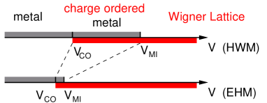
Figure 1: Sketched phase diagram of the quarter-filled Hubbard-Wigner model. The uniform metallic phase is stabilized by the inclusion of long-range Coulomb interactions (HWM) compared to the model with short range interactions (EHM) and an intermediate charge ordered metallic phase emerges in between the uniform metal and the Wigner lattice.

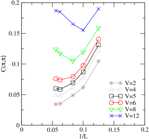
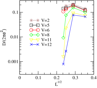
Figure 2: Finite-size scaling of the static charge correlation function evaluated at $(\pi,\pi)$ (a) and Drude weight (b) for different values of $V$. The charge ordering transition is estimated to occur at $V_{CO}\approx 4t$ from the linear extrapolation to the thermodynamic limit of $C(\pi,\pi)$ vs. $1/L$. The Drude weight is plotted as a function of $1/\sqrt{L}$, displaying insulating behavior for $V>V_{MI}\approx 8t$.

The phase diagram of the HWM obtained from exact diagonalization (ED) of finite-size clusters is illustrated in Fig. 1, where two distinct phase transitions can be identified. The first one corresponds to the charge ordering instability of the homogeneous metal, indicated by the presence of non-zero charge correlations at the critical wavevector ${\bf Q}=(\pi,\pi)$. In Fig. 2 (a) we show the finite size scaling of the charge correlation function on $L=8,10,16,18$ clusters as a function of $1/L$. The extrapolation to the thermodynamic limit suggests a charge ordering transition at about $V_{CO}\approx(4-5)t$ in good agreement with previous results using the Path Integral Renormalization Group (PIRG) on $4\times 4$, $8\times 8$ and $12\times 12$ clusters (see Fig. 2 and Ref. Imada2, ). This value is much larger than the $1.5t$ obtained for the EHM (see also Ref. Calandra02, ). This indicates that the uniform metallic phase is notably stabilized by the inclusion of long-range interactions Tsiper ; Imada2 . To trace back the physical origin of this phenomenon, we observe that the CO instability can be understood through the divergence of the charge susceptibility in the Random Phase Approximation (RPA): $\chi_{c}({\bf Q})=\chi_{0}({\bf Q})/\left[1+V({\bf Q})\chi_{0}({\bf Q})\right]$ with $\chi_{0}({\bf Q})$ the bare susceptibility independent of the Coulomb repulsion and $V({\bf Q})$ the interaction potential in reciprocal space at wavevector ${\bf Q}$. Since the absolute value of $V({\bf Q})$ in the model with long-range interactions is much reduced (by a factor of $2.5$) as compared to the case with nearest-neighbor interactions alone, the above argument predicts $V_{CO}\simeq 4t$ in the HWM, in agreement with the ED result. Remarkably, the three different estimates based on ED, PIRG and the RPA scaling argument lead to the same value of $V_{CO}$. This result obtained by considering the full long-range Coulomb potential already settles a long-standing puzzle in quarter-filled layered organic conductors, many of which are found to be metallic even for values of $V$ comparable or larger than the bandwidth of the material.

The second critical point corresponds to the metal-insulator transition, signaled by the vanishing of the Drude weight. The finite-size scaling of this quantity is shown in Fig. 2 (b). The Drude weight displays a large drop at about $V_{MI}\approx(7-8)t$ after extrapolating to the thermodynamic limit. The broad region $V_{CO}<V<V_{MI}$ therefore corresponds to a charge ordered, metallic phase. This phase, which can be easily discerned from a metallic CDW (see below), might be intimately related to the hybrid phase predicted at the quantum melting of the Wigner crystal in the continuum. Spivak ; Waintal The robustness of the COM phase can indeed be contrasted to the model with short range interactions, where a rather narrow intermediate region (if any) arises: between $V_{CO}\simeq 1.5t$, and $V_{MI}\simeq 1.8t$ also consistent with the COM found with cluster dynamical mean-field theory CDMFT . Spin correlations are also enhanced in the same parameter range, suggesting that charge and spin do order together in the metallic phase before the metal-insulator transition occurs. Such spin order corresponds to antiferromagnetism between charge rich sites due to “ring” exchange processes McKenzie2 . It can be noted that using a more realistic value of $U=20t$ significantly increases the value of $V_{MI}$, while leaving $V_{CO}$ essentially unchanged, which effectively broadens the region of stability of the COM phase.

III.2 Excitation spectra

As we proceed to show, the charge ordered metallic phase found here shares common aspects of both Mott and Wigner physics. Its anomalous properties are a direct manifestation of the collective nature of its low-lying excitations, originating from the long-range Coulomb repulsion as well as the strong correlation effects associated with the on-site Coulomb interaction in a narrow-band system. To characterize the excitation spectrum we now introduce two representative quantities: the single-particle charge gap $\Delta_{ch}$ measured in photoemission experiments, that represents the energy required to add/remove an electron to/from the system; the optical gap $\Delta_{opt}$ defined as the the lowest charge excitation allowed by the dipolar matrix element, corresponding to the onset of finite-frequency absorption in an optical experiment. The former carries information on the one-particle excitations, the latter gives access to the local charge fluctuations, pertaining to the collective sector of the spectrum. While such quantities coincide for non-interacting electrons, their comparison in an interacting system provides valuable information on the excitation spectrum. These quantities are plotted in Fig. 3(a) and (b) respectively for the EHM and HWM in an $L=16$ cluster, and allow us to analyze the relative role played by the single particle against the collective excitations.

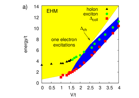
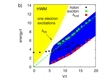
Figure 3: (Color online) Excitation spectra for the models with (a) nearest neighbor (EHM) and (b) long-range interactions (HWM) on $L=16$ sites. The symbols represent respectively the holon (triangles) and exciton (dots) peaks in the optical conductivity, and the lowest excitation of finite energy as given by the ED (squares). The light shaded (yellow) region is delimited by the single-particle charge gap $\Delta_{ch}$, while the dark (blue) region corresponds to the collective excitations of the Wigner lattice, bounded from below by $\Delta_{coll}$. The dashed line is the predicted exciton energy in the thermodynamic limit, $0.62V$ (see the appendix).

Let us consider the EHM first. At large $V\gg t$ the charges order in the checkerboard pattern shown in Fig. 4. The process of adding an electron or a hole (Fig. 4a) defines the one-particle charge gap $\Delta_{ch}=4V$. Reducing the interaction strength leads to a progressive closing of $\Delta_{ch}$ (the boundary of the yellow region in Fig. 3a), that eventually triggers the metallization transition and the consequent melting of the charge ordered state. In addition to the usual one-particle excitations, the motion of a particle in the EHM from the perfect checkerboard pattern to one of its neighboring unoccupied sites gives rise to a local (neutral) charge fluctuation depicted in Fig. 4b. The latter costs an energy $\Delta_{opt}=3V$, which at large $V$ lies below the single-particle gap. As $V/t$ decreases, however, the quasiparticle excitations rapidly take over owing to their large kinetic energy gain $\sim 8t$. As can be seen in Fig. 3a, in the region around $V_{MI}$ there is no longer a clear-cut distinction between the one-electron and the collective sectors, and the neutral charge fluctuations do not play a major role in the transition mechanism. In fact, the critical point in the case of short range interactions can be estimated by comparing $\Delta_{ch}$ with the bandwidth $\approx 8t$: this qualitative argument yields $V_{MI}\lesssim 2t$ (the $\lesssim$ sign accounts for the bandwidth reduction due to the local $U$), in agreement with the numerical result $V_{MI}\simeq 1.8t$.

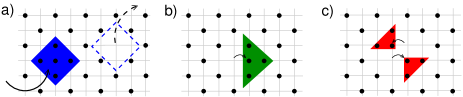
Figure 4: (Color online) Lowest-energy excitations of the checkerboard Wigner lattice: (a) Charged (monopoles), (b) neutral (dipolar) and (c) (quadrupolar) defects. (a) corresponds to the process of adding/removing a particle to form an interstitial/vacancy, which determines the charge gap $\Delta_{ch}=1.62V$; (b) is a local (dipolar) charge fluctuation of energy $\Delta_{opt}=0.62V$, that can be viewed as a tightly bound interstitial-vacancy pair, or an exciton; (c) is the next (quadrupolar) excitation of energy $\Delta_{quad}=0.65V$.

This picture changes drastically when the full long-range Coulomb repulsion is included, as in the Hubbard-Wigner model Eq. (1). The key point is that in this case the defects of the checkerboard pattern are no longer confined. Andreev Since the electrostatic energy is essentially insensitive to local details, being mostly determined by the long-range tails of the Coulomb potential, several electronic configurations can be found which are almost degenerate with the local defect of Fig. 4b. For example, the energy of the quadrupolar excitation shown in Fig. 4c is only $0.03V$ larger than that of Fig. 4b, making these two states practically degenerate for any realistic value of $V$. As a result, the electron can resonate between these states, forming a “charge droplet” that can propagate coherently at long distances with a net kinetic energy gain $\propto t$. This phenomenon is directly reflected in the excitation spectrum shown in Fig. 3b: a collective, itinerant defect state emerges well below both the optical gap $\Delta_{opt}$ and the charge gap $\Delta_{ch}$, whose energy $\Delta_{coll}\simeq\Delta_{opt}-4.2t$ qualitatively agrees with the prediction of the defect model, $\Delta_{coll}\simeq\Delta_{opt}-2\sqrt{2}t$ derived in the appendix.

We see that due to the delocalization of defects in the presence of long-range interactions, these collective excitations can gain a kinetic energy comparable to the one-particle excitations. As a result, the separation of energy scales between the collective sector and the single-particle sector, characteristic of the strongly interacting limit, survives down to $V_{MI}$ and below. Accordingly, the metallization transition as well as the resulting charge ordered metallic phase in the region $V_{CO}<V<V_{MI}$ appear to be entirely driven by the low-energy collective sector Tsiper . The finite-size scaling shown in Fig. 5 strongly suggests that the one-particle charge gap $\Delta_{ch}$ remains finite within the metallic phase: the charge gap is found to open concomitantly with the charge ordering transition occurring at $V_{CO}\approx 4t<V_{MI}$, i. e. in the range of parameters where the system has a non-zero Drude weight. The region $V_{CO}<V<V_{MI}$ therefore corresponds to a charge ordered, metallic phase, with a vanishing single-particle weight at low energy.

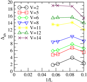
Figure 5: Finite-size scaling of the single-particle charge gap, $\Delta_{ch}$, for different cluster sizes. Linear extrapolation to the thermodynamic limit indicates that the charge gap opens at $V\approx 4t\approx V_{CO}<V_{MI}$ suggesting a phase with a finite charge gap, charge order and non-zero Drude weight (see also Fig. 2).

III.3 Spectral probes

The excitation spectrum described in the preceding paragraphs provides a way to univocally characterize the anomalous COM phase predicted here. First of all, in conjunction with the charge ordering observed by X-ray diffraction or NMR, photoemission or tunneling experiments should find a finite single-particle gap (see Figs. 3b and 5), despite a markedly metallic behavior. In fact both the large value of the charge gap as well as the energy dispersion of the lowest-lying single-particle excitations are well captured by the defect model presented in the appendix. There it is shown that the dispersion of the charged interstitials of Fig. 4a is accurately described by the following formula:

$$E_{k} = E_{0}-2t_{1}[\cos(2k_{x})+\cos(2k_{y})]$$

$$-2t_{2}[\cos(k_{x}+k_{y})+\cos(k_{x}-k_{y})].$$

representing the motion of interstitials respectively along the principal axes and along the diagonals of the square lattice. The physical picture that emerges from the dispersion relation Eq.(III.3) is that of interstitial defects moving as a separate fluid on top of the charge ordered pattern, which bears a strong resemblance with the hybrid phase of the Wigner crystal in the continuum.Waintal An important implication of the defect model is that the hopping parameters $t_{1},t_{2}$ governing the motion of interstitials are essentially constant throughout the charge ordered phase: the one-electron band dispersion depends on the interaction strength $V$ only via the rigid energy shift $E_{0}$, related to the charge gap $\Delta_{ch}$. This can once again be contrasted with the standard CDW picture where the band dispersion shrinks as $\propto t^{2}/V$ upon increasing $V$.

Fig.6 shows the spectral function $A(k,\omega)$ obtained from the exact diagonalisation of a $L=16$ cluster for $V=10t$, which lies well within the charge ordered metallic phase for this system size. The main peak clearly follows the dispersion of the defect band [Eq. (III.3), with $t_{1}=0$, $t_{2}=-0.3t$] representing the motion of interstitials along the diagonals of the square lattice. A similar agreement applies throughout the charge ordered metallic phase $V_{CO}<V<V_{MI}$, improving at larger values of $V$.

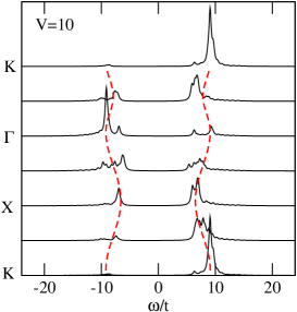
Figure 6: The spectral function $A(k,\omega)$ as obtained from Lanczos diagonalisation of the Hubbard-Wigner model on a $L=16$ cluster at $V/t=10$. The different points in the Brilloun zone are $\Gamma=(0,0)$, $X=(\pi,0)$, $K=(\pi,\pi)$. The red dashed line is the band dispersion Eq. (III.3) of defects moving along the diagonals of the square lattice. The offset energy $E_{0}$ has been adjusted to fit the overall position of the bands. Note that the critical values $V_{CO}$ and $V_{MI}$ at this system size are larger than those extrapolated to the thermodynamic limit, so that the value $V/t=10$ is representative of the charge ordered metallic region $V_{CO}<V<V_{MI}$.

The calculated optical conductivity also reveals clear signatures of the predicted COM phase. As shown in Fig. 7(a), in addition to a Drude peak (presumably anomalous, being possibly carried by collective excitations), the optical spectra exhibit two distinct finite-frequency absorption bands, confirming the ’mixed’ nature of such intermediate phase: a low-frequency ’holon’ peak at about $(3-4)t$ originating from the short-range correlations, and enhanced by the non-local Coulomb repulsion Greco ; Dressel , plus a broader excitonic band at $\Delta_{opt}=0.62V$, corresponding to the dipolar defects of the Wigner lattice. Fig. 7(b) shows the integrated optical spectra, $I(\omega)$, across the CO transition. For $V=0$, most of the spectral weight is in the Drude weight and $I(\omega)$ saturates rapidly with $\omega$. As $V$ increases a strong redistribution of spectral weight occurs with the low energy optical weight being transfered to higher energies (of the order of $\Delta_{opt}$). The total integrated spectrum is a measure of the kinetic energy of the system as derived from the $f$-sum ruleMaldague . Fig. 7(b) shows how the electron kinetic energy is suppressed by $V$ due to electron correlation effects close to the CO transition.

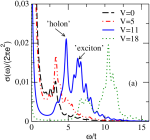
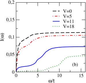
Figure 7: (Color online) Optical properties across the CO transition in the Hubbard-Wigner model. (a) The ’holon’ absorption band of the strongly correlated metal is strongly enhanced by $V$, dominating the optical conductivity spectra for $V<V_{CO}$. Within the charge ordered metallic phase, $V_{CO}<V<V_{MI}$ a broader band at about $0.62V$ arises due to bound excitons (Fig. 4b). (b) Integrated spectral weight of the optical conductivity for the same parameters as in (a). A strong transfer of spectral weight from low energies to high energies across the CO transition is evident. Results are shown for a $L=16$ cluster.

IV Concluding remarks

The quarter-filled layered organic crystals of the $\theta$-type are ideal realizations of a Wigner lattice in which some of the existing experiments could be interpreted in light of the present scenario. The horizontal charge ordered pattern observed through X-rays Mori07 below the CO temperature $T_{CO}=190$K in $\theta$-(ET)₂RbZn(SCN)₄, is consistent with CO driven by the off-site Coulomb repulsion but inconsistent with any Fermi surface nesting vector. In the metallic salt $\theta$-(ET)₂CsZn(SCN)₄, both stripe-type and three-fold CO patterns are observed, both related to strong off-site Coulomb repulsion Mori07 . Metallic phases above $T_{CO}$ display ’bad’ metallic behavior with very weak $T$-dependence and absolute values much larger than the Mott-Ioffe-Regel limit Mori98 indicating mean free paths much smaller than the lattice parameter. On application of an electric field to $\theta$-(ET)₂CsCo(SCN)₄, charge order is melted and the conductivity is increased by several orders of magnitude Sawano .

All the above observations suggest that an unconventional metallic phase might be realized in such materials at the melting of the Wigner lattice driven by quantum fluctuations, which should be further experimentally probed. Such a metal should display a charge gap in one-electron probes such as photoemission or STM, or a large pseudogap on the scale of the non-local Coulomb energy V Vlad , together with metallic conduction due to the itinerancy of defects in the charge ordered background. The enhancement of charge fluctuations in the intermediate metallic phase could mediate superconductivity MM close to the charge ordering instability occurring, for example, in $\theta$-type layered organic conductors and NbSe₃ Kiss . Elucidating the precise nature of the current-carrying excitations emerging at zero energy in such anomalous COM phase remains an open challenge, as is the understanding of the interplay between the Mott and Wigner mechanisms for the metal-insulator transition. Camjayi08

Appendix A Defect deconfinement in the Wigner lattice

A system of electrons is expected to crystallize when the mutual Coulomb interactions dominate over the kinetic energy. Minimizing the electrostatic interaction energy in a two-dimensional electron gas results in a triangular arrangement of the charges. The preferred triangular ordering is altered by the presence of an underlying periodic potential in a solid: Uimin ; Cocho ; Fate for a density of $n=1/2$ electrons per site on a square host lattice the configuration of minimal electrostatic energy is the checkerboard order shown in Fig.4. We designate such “Wigner crystal on an underlying host lattice” simply as a Wigner lattice (WL).

As we show below, the physics of the Wigner lattice in the strongly interacting regime $V\gg t$ can be effectively understood by considering only a small number of defects of the classical checkerboard, which play a dominant role in the low-energy excitation spectrum. These defects can be separated in two different classes. The first class corresponds to fluctuations of the charge density induced by quantum fluctuations in the presence of a non-vanishing transfer integral $t\neq 0$, that will be denoted as neutral collective excitations. Excitations of the second class, termed charged one-particle excitations arise when an extra charge is added/removed to/from the system, which is the typical situation in a photoemission experiment. In the following paragraphs we analyze the two categories separately.

A.1 Neutral, collective excitations

In the limit of strong Coulomb interactions $V\gg t$, the excitations of the Wigner lattice can be classified in terms of the potential (Madelung) energy of the electronic configurations. The lowest-energy excitations of the checkerboard pattern are the dipolar and quadrupolar defects illustrated in Fig.4b and c. These are obtained by moving respectively one or two electrons away from their preferred equilibrium position, as shown by the arrows. The corresponding electrostatic energies can be evaluated to arbitrary accuracy through standard Ewald summations, being $\Delta_{opt}=0.6155V$ and $\Delta_{quad}=0.6453V$. The next electronic configurations (not shown) have energies $\geq 0.898V$ and will be discarded in the following discussion.

Using the procedure of Ref. Rast , we calculate the energy gain induced by a finite transfer integral $t$ between molecular sites. This is achieved by restoring the translational invariance and solving the tight-binding problem in Fourier space within the reduced subspace consisting of the two defects described above. Accounting for the two possible orientations of the quadrupolar defect and the four orientations of the dipolar defect, we are led to diagonalise the following $6\times 6$ matrix (the intermolecular spacing $a$ is taken as the unit length):

$$\left(\begin{array}[]{cccccc}\Delta_{quad}&0&-te^{ik_{x}}&-te^{-ik_{x}}&-te^{ik_{y}}&-te^{-ik_{y}}\\ 0&\Delta_{quad}&-te^{-ik_{x}}&-te^{ik_{x}}&-te^{-ik_{y}}&-te^{ik_{y}}\\ -te^{-ik_{x}}&-te^{ik_{x}}&\Delta_{opt}&0&0&0\\ -te^{ik_{x}}&-te^{-ik_{x}}&0&\Delta_{opt}&0&0\\ -te^{-ik_{y}}&-te^{ik_{y}}&0&0&\Delta_{opt}&0\\ -te^{ik_{y}}&-te^{-ik_{y}}&0&0&0&\Delta_{opt}\end{array}\right)$$ (3)

The key point here is that due to the long-range nature of the electron-electron interactions, the dipolar and quadrupolar defects are almost degenerate in energy: $\Delta_{quad}-\Delta_{opt}\simeq 0.03V$. As a result a resonant tunneling is established between the two non-equivalent states for any physically reasonable value of the $V/t$ ratio. The electron density is then shared between these states, forming an “electron droplet”. Such delocalisation of the charge yields a kinetic energy gain $\propto t$ and allows the droplet to propagate coherently at long distances with a band-like dispersion. The present scenario can be contrasted to the model with nearest-neighbour interactions, where the defects remain strongly localized in space unless the transfer integral overcomes the large energy barrier separating the states depicted in Figs. 4b and c, i.e. $t\gtrsim(\Delta_{quad}-\Delta_{opt})=V$.

By setting $\Delta_{quad}=\Delta_{opt}$ in the matrix (3) we obtain an analytical expression for the energy gain of the droplet state at $k=0$:

$$\Delta_{k=0}=\Delta_{opt}-2\sqrt{2}t.$$ (4)

This form is in satisfactory agreement with the exact diagonalization (ED) result: $\Delta_{k=0}\simeq\Delta_{opt}-4.2t$, indicating that the physical mechanism of defect delocalization is correctly captured already in the small droplet approximation, where only dipolar and quadrupolar states are included.

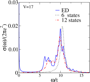
Figure 8: (Color online) Comparison of the optical conductivity calculated at $V=17t$ from ED of a $L=16$ cluster with the one obtained from the defect model, including respectively the 6 and 12 lowest-lying states.

We note that while the quadrupolar states are the ones responsible for the band dispersion, it can be shown following the lines of Ref. Rast that the optical spectral weight is mostly carried by the dispersionless dipolar excitations. As a result, the peak in the optical conductivity remains centered at an energy $\omega=\Delta_{opt}$ while the peak at $\omega=\Delta_{k=0}$ is not optically active. The optical conductivity calculated from the defect model at $V=17t$ is shown in Fig. 8, and compared with the spectrum obtained from the full ED in a $L=16$ cluster. The minimal model of Eq. (3) including 6 defect states is able to reproduce the correct position of the exciton peak. Extending the defect subspace to a total of 12 states also accounts for the emergence of a sideband below the main peak, as seen in the numerical data.

A.2 Charged, single particle excitations: interstitials and vacancies

An analogous procedure can be carried out to determine the dispersion of the one-electron states that are probed in photoemission experiments. It is convenient to include a static compensating charge density of $+e/2$ per site in the calculation (equivalent to the usual compensating jellium in continuum models), which restores the overall charge neutrality and the particle-hole symmetry. We can therefore focus on the addition spectrum alone, since the removal spectrum is obtained by symmetry.

As usual we start from the $V\gg t$ limit. Adding an electron to an empty site of the Wigner lattice creates an interstitial, of energy $E_{I}=0.8078V$. The next low-lying states with $N+1$ electrons have energies respectively $E_{D}=0.9233$ and $E_{M}=1.1304$. All these states are illustrated in Fig.9. The charge gap is defined as $\Delta_{ch}=E(N+1)+E(N-1)-2E(N)$ which gives $\Delta_{ch}=2|E_{I}|=1.6155V$.

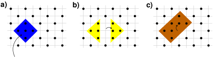
Figure 9: The lowest-lying states with one electron added to the perfect checkerboard pattern. From left to right the corresponding Madelung energies in an infinite system are (a) $E_{I}=0.8078V$, (b) $E_{D}=0.9233$ and (c) $E_{M}=1.1304$.

In order to study the effect of quantum fluctuations induced by a finite transfer integral $t$ we evaluate the action of the kinetic energy operator within the subspace of the defect states defined above. Considering the multiplicities arising from the possible orientations of these states (respectively $2,4,8$) one obtains the $14\times 14$ matrix shown in Table 2. The charge gap at finite $t$ is obtained from the energy of the lowest state at $k=0$. In the region $10<V/t<20$ it follows the linear form $\Delta_{ch}\simeq 1.8V-9.6t$, in good agreement with the ED value: $\Delta_{ch}\simeq 1.8V-7.0t$.

To get more insight on the one-particle excitations of the Wigner lattice, we observe that the bands arising from the diagonalization of the matrix in Table 2 are accurately described by the following formula:

$$E_{k} = E_{0}-2t_{1}[\cos(2k_{x})+\cos(2k_{y})]$$

$$-2t_{2}[\cos(k_{x}+k_{y})+\cos(k_{x}-k_{y})].$$

An important implication of the defect model is that the hopping parameters $t_{1},t_{2}$ governing the motion of defects are essentially constant throughout the charge ordered phase: the one-electron band dispersion depends on the interaction strength $V$ only via the rigid energy shift $E_{0}$. For a direct validation of the defect model, Fig.6 shows how the spectral function $A(k,\omega)$ obtained from the exact diagonalisation of a $L=16$ cluster within the charge ordered metallic phase closely follows the dispersion of the main defect band [Eq. (A.2), with $t_{1}=0$, $t_{2}=-0.3t$], which represents the motion of interstitials along the diagonals of the square lattice.

Appendix B Finite-size effects

As was pointed out in Ref.Tsiper , in addition to the usual size effects encountered in numerical studies of model systems on finite clusters (hereafter denoted as quantum finite-size effects), specific issues arise when dealing with the long-range Coulomb potential. These originate from the inaccuracy of calculating the electrostatic energy of the electronic configurations in a finite system. Such effects are termed classical finite size effects and become relevant within the charge ordered phase at large $V/t$.

B.1 Quantum finite-size effects

Ordinary finite size effects in the EHM have been explored previously by comparing results of different quantities with different number of cluster sites $L=8,10,16$ and $20$Calandra02 . Other possible ways of evaluating finite size effects are based on averaging over the boundary condition Koretsune . In the case of the extended Hubbard model both procedures are found to lead to similar critical valuesSeo .

We have performed finite-size scaling for the HWM by evaluating the charge correlation function, $C(\pi,\pi)$, Drude weight, $D$, and charge gap, $\Delta_{ch}$ on $L=8,10,16,18$ clusters, and analyzing the extrapolation to the thermodynamic limit. In Fig. 2 we show $C(\pi,\pi)$ plotted as a function of $1/L$ and the Drude weight, $D$, dependence with $1/\sqrt{L}$. The finite size scaling of the single particle charge gap, $\Delta_{ch}$, is shown in Fig. 5. Our finite-size scaling analysis strongly suggests the presence of a broad metallic phase with both charge order and a finite single-particle charge gap for $V_{CO}<V<V_{MI}$.

B.2 Classical finite-size effects

Classical finite-size effects are minimized by evaluating electrostatic energies with Ewald summations, which amounts to performing an infinite periodic repetition of the finite simulation cell. Although a system of infinite size is effectively recovered through this procedure, this gives rise to spurious contributions to the energy arising from the interaction of a given electronic configuration with its images on the repeated cells. Since the simulation cell is overall neutral, the interaction between equivalent cells has a dipolar nature and the corresponding error in the energy scales at most as $\Delta E\sim V/L^{3/2}$ ($L$ being the total number of sites).

Having identified in Appendix A those electronic configurations that are mainly responsible for the low-energy behaviour of the Wigner lattice, we can precisely address the effect of such uncertainties on the physics of interest here. To this aim we report in Table 1 the electrostatic energies of the configurations used in the defect model of Appendix A, and compare them with the corresponding values in a $4\times 4$ cluster (energies are expressed in units of $V$). As we can see, finite-size errors on these states are typically of the order of $5-10\%$ or less, which gives us good confidence on the final numerical results.

$$\begin{array}[]{|c|ccccc|}\hline\cr&E_{opt}&E_{quad}&E_{I}&E_{D}&E_{M}\\ \hline\cr extended&0.6155&0.6453&0.8078&0.9233&1.1304\\ 4\times 4&0.5776&0.6258&0.8078&1.0370&1.1207\\ \hline\cr\end{array}$$

Table 1: Electrostatic energies of the relevant defect states.

Table 2: The $14\times 14$ matrix used to calculate the one-particle excitation spectrum in the defect subspace.

$$\left(\begin{array}[]{cccccccccccccc}E_{I}&0&-2t\cos k_{x}&-2t\cos k_{y}&0&0&-te^{i\frac{k_{x}+k_{y}}{2}}&-te^{i\frac{k_{x}+k_{y}}{2}}&-te^{-i\frac{k_{x}+k_{y}}{2}}&-te^{-i\frac{k_{x}+k_{y}}{2}}&-te^{-i\frac{k_{x}-k_{y}}{2}}&-te^{-i\frac{k_{x}-k_{y}}{2}}&-te^{i\frac{k_{x}-k_{y}}{2}}&-te^{i\frac{k_{x}-k_{y}}{2}}\\ 0&E_{I}&-2t\cos k_{x}&-2t\cos k_{y}&0&0&-te^{-i\frac{k_{x}+k_{y}}{2}}&-te^{-i\frac{k_{x}+k_{y}}{2}}&-te^{i\frac{k_{x}+k_{y}}{2}}&-te^{i\frac{k_{x}+k_{y}}{2}}&-te^{i\frac{k_{x}-k_{y}}{2}}&-te^{i\frac{k_{x}-k_{y}}{2}}&-te^{-i\frac{k_{x}-k_{y}}{2}}&-te^{-i\frac{k_{x}-k_{y}}{2}}\\ -2t\cos k_{x}&0&E_{D}&0&0&0&0&0&0&0&0&0&0&0\\ -2t\cos k_{y}&0&0&E_{D}&0&0&0&0&0&0&0&0&0&0\\ 0&-2t\cos k_{x}&0&0&E_{D}&0&0&0&0&0&0&0&0&0\\ 0&-2t\cos k_{y}&0&0&0&E_{D}&0&0&0&0&0&0&0&0\\ -te^{-i\frac{k_{x}+k_{y}}{2}}&-te^{i\frac{k_{x}+k_{y}}{2}}&0&0&0&0&E_{M}&0&0&0&0&0&0&0\\ -te^{-i\frac{k_{x}+k_{y}}{2}}&-te^{i\frac{k_{x}+k_{y}}{2}}&0&0&0&0&0&E_{M}&0&0&0&0&0&0\\ -te^{i\frac{k_{x}+k_{y}}{2}}&-te^{-i\frac{k_{x}+k_{y}}{2}}&0&0&0&0&0&0&E_{M}&0&0&0&0&0\\ -te^{i\frac{k_{x}+k_{y}}{2}}&-te^{-i\frac{k_{x}+k_{y}}{2}}&0&0&0&0&0&0&0&E_{M}&0&0&0&0\\ -te^{i\frac{k_{x}-k_{y}}{2}}&-te^{-i\frac{k_{x}-k_{y}}{2}}&0&0&0&0&0&0&0&0&E_{M}&0&0&0\\ -te^{i\frac{k_{x}-k_{y}}{2}}&-te^{-i\frac{k_{x}-k_{y}}{2}}&0&0&0&0&0&0&0&0&0&E_{M}&0&0\\ -te^{-i\frac{k_{x}-k_{y}}{2}}&-te^{i\frac{k_{x}-k_{y}}{2}}&0&0&0&0&0&0&0&0&0&0&E_{M}&0\\ -te^{-i\frac{k_{x}-k_{y}}{2}}&-te^{i\frac{k_{x}-k_{y}}{2}}&0&0&0&0&0&0&0&0&0&0&0&E_{M}\end{array}\right)$$

References

- (1) M. Imada, A. Fujimori, and Y. Tokura, Rev. Mod. Phys. 70 1039 (1998).
- (2) E. Wigner, Phys. Rev. 46, 1002 (1934).
- (3) D. A. Bonn, Nature Phys. 2, 159 (2006).
- (4) P. A. Lee, Rep. Prog. Phys. 71 012501 (2008).
- (5) T. Ishiguro, K. Yamaji, and G. Saito, Organic superconductors. (Springer, 2nd Edition, 2001).
- (6) R. H. McKenzie, Science 278, 820 (1997).
- (7) S. V. Kravchenko, and M. P. Sarachik, Rep. Prog. Phys. 67, 1 (2004).
- (8) E. Abrahams, S. V. Kravchenko, and M. P. Sarachik, Rev. Mod. Phys. 73, 251-266 (2001).
- (9) J. Hubbard, Phys. Rev. B 17, 494 (1978).
- (10) H. Seo, J. Merino, H. Yoshioka, and M. Ogata, Jour. Phys. Soc. Jap. 75 051009 (2006).
- (11) S. Pankov and V. Dobrosavljević, Phys. Rev. B 77, 085104 (2008).
- (12) A. Camjayi, K. Haule, V. Dobrosavljević, and G. Kotliar, Nature Phys. 4, 932 (2008)
- (13) B. Valenzuela, S. Fratini, and D. Baeriswyl, Phys. Rev. B 68, 045112 (2003)
- (14) S. Fratini, B. Valenzuela, and D. Baeriswyl, Synth. Met. 141, 193 (2004)
- (15) M. Mayr and P. Horsch, Phys. Rev. B 73, 195103 (2006)
- (16) M. Daghofer and P. Horsch, Phys. Rev. B 75, 125116 (2007).
- (17) E. V. Tsiper and A. L. Efros, Phys. Rev. B 57, 6949 (1998)
- (18) F. Pollmann, J. J. Betouras, K. Shtengel, and P. Fulde, Phys. Rev. Lett. 97, 170407 (2006)
- (19) M. Calandra, J. Merino and R. H. McKenzie, Phys. Rev. B 66, 195102 (2002).
- (20) Y. Noda and M. Imada, Phys. Rev. Lett. 89 176803 (2002).
- (21) B. Spivak and S. Kivelson, Phys. Rev. B 70 155114 (2004)
- (22) H. Falakshashi and X. Waintal, Phys. Rev. Lett. 94, 046801 (2005).
- (23) J. Merino, Phys Rev. Lett. 99 036404 (2007).
- (24) R. H. McKenzie, J. Merino, J. B. Marston, and O. P. Sushkov, Phys. Rev. B 64 085109 (2001).
- (25) Y. Bang and G. Kotliar, Phys. Rev. B 48 9898 (1993).
- (26) A. F. Andreev and L. M. Lifshitz, Sov. Phys. JETP 29, 1107 (1969)
- (27) J. Merino, A. Greco, R. H. McKenzie, and M. Calandra, Phys. Rev. B 68, 245121 (2003).
- (28) M. Dressel, N. Drichko, J. Schlueter, and J. Merino, Phys. Rev. Lett. 90, 167002 (2003).
- (29) P. F. Maldague, Phys. Rev. B 16 2437 (1977).
- (30) T. Mori, I. Terasaki, and H. Mori, Jour. Mat. Chem.17 1 (2007), and references therein.
- (31) H. Mori, S. Tanaka, and T. Mori, Phys. Rev. B 57 12023 (1998).
- (32) F. Sawano, I. Terasaki, H. Mori, T. Mori, M. Watanabe, N. Ikeda, Y. Nogami, Y. Noda, Nature 437, 522 (2005)
- (33) S. Pankov and V. Dobrosavljevic, Phys. Rev. Lett. 94, 046402 (2005)
- (34) J. Merino and R. H. McKenzie, Phys. Rev. Lett. 87 237002 (2001).
- (35) T. Kiss, T. Yokoya, A. Chainani, S. Shin, T. Hanaguri, M. Nohara and H. Takagi, Nature Phys. 3 720 (2007).
- (36) V. L. Pokrovsky and G. V. Uimin, J. Phys. C 11, 3535 (1978)
- (37) G. Cocho, R. Pérez Pascual and J. L. Rius, Europhys. Lett. 2, 493 (1986)
- (38) D. Baeriswyl and S. Fratini, J. Phys. IV France 131, 247 (2005)
- (39) S. Fratini and G. Rastelli, Phys. Rev. B 75, 195103 (2007)
- (40) T. Koretsune, Y. Motome, and A. Furusaki, Jour. Phys. Soc. Jap. 76 074719 (2007).