Suzaku Wide Band Analysis of the X-ray Variability of TeV Blazar Mrk 421 in 2006

Abstract

We present the results of X-ray observations of the well-studied TeV blazar Mrk 421 with the Suzaku satellite in 2006 April 28. During the observation, Mrk 421 was undergoing a large flare and the X-ray flux was variable, decreasing by $\sim 50$ %, from $7.8\times 10^{-10}$ to $3.7\times 10^{-10}$ erg s^-1cm^-2 in about 6 hours, followed by an increase by $\sim 35$ %. Thanks to the broad bandpass coupled with high-sensitivity of Suzaku, we measured the evolution of the spectrum over the 0.4–60 keV band in data segments as short as $\sim 1$ ksec. The data show deviations from a simple power law model, but also a clear spectral variability. The time-resolved spectra are fitted by a synchrotron model, where the observed spectrum is due to a exponentially cutoff power law distribution of electrons radiating in uniform magnetic field; this model is preferred over a broken power law. As another scenario, we separate the spectrum into “steady” and “variable” components by subtracting the spectrum in the lowest-flux period from those of other data segments. In this context, the difference (“variable”) spectra are all well described by a broken power law model with photon index $\Gamma\sim 1.6$, breaking at energy $\epsilon_{\rm brk}\simeq 3$ keV to another photon index $\Gamma\sim 2.1$ above the break energy, differing from each other only by normalization, while the spectrum of the “steady” component is best described by the synchrotron model. We suggest the rapidly variable component is due to relatively localized shock (Fermi I) acceleration, while the slowly variable (“steady”) component is due to the superposition of shocks located at larger distance along the jet, or due to other acceleration process, such as the stochastic acceleration on magnetic turbulence (Fermi II) in the more extended region.

1. Introduction

Blazars, a sub-category of Active Galactic Nuclei (AGN), are characterized by broadband non-thermal emission and violent variability on time scales from a fraction of an hour to a few days with strong spectral evolution. This behavior is best described as their emission arising from Doppler-boosted relativistic jets which in turn dominates over the thermal signatures seen in other AGN (e.g., Urry & Padovani, 1995; Ulrich et al., 1997). The broadband spectra of blazars consist of two peaks, one in the radio to optical–UV range (and in some cases, reaching to the X-ray band), and the other in the hard X-ray to $\gamma$-ray region. The high polarization of the radio to optical emission suggests that the lower energy peak is produced via the synchrotron process by relativistic electrons in the jet (see, e.g., Angel & Stockman, 1980). The higher energy peak is believed to be due to Compton up-scattering of seed photons by the relativistic electrons. A number of blazars with the synchrotron peak located in the X-ray range have also been detected in the TeV band, and the recent advances of TeV Cherenkov telescopes have revealed the existence of significant number of such TeV emitting blazars (see Wagner et al., 2008, for recent synoptic study). These objects provide the most direct evidence of efficient particle acceleration up to TeV energies, potentially providing the key information about the jet’s composition and power, and thus the connection of it the central engine.

Mrk 421 is one of the nearest (z=0.031) and brightest TeV $\gamma$-ray emitting blazars: it was found as the first extragalactic TeV $\gamma$-ray emitting object (Punch et al., 1992), and has been repeatedly confirmed as a TeV source by various ground-based telescopes (e.g., Aharonian et al., 2005; Albert et al., 2007). It has also been one of the most extensively studied blazars, and has been a target of several multi-wavelength campaigns (e.g., Takahashi et al., 1996, 2000; Tosti et al., 1998; Rebillot et al., 2006; Fossati et al., 2008; Lichti et al., 2008). Detailed studies during large amplitude flares are particularly important as they give us vital information allowing studies of the underlying physics of the source. In particular, the simultaneous observations in X-ray and TeV $\gamma$-ray band revealed a strong correlation between them and depict the picture in which the non-thermal distribution of relativistic electrons accelerated up to TeV energies are responsible for the variability of both bands. Such a scenario - where lower energy component is synchrotron radiation from the relativistically accelerated electrons and the higher energy one is due to Compton up-scattering of the synchrotron photons by the same electron populations themselves - is widely adopted as the most plausible emission mechanism for TeV blazars, and is called one-zone Synchrotron Self-Compton (SSC) model (Inoue & Takahara, 1996; Kataoka et al., 1999).

Although the simplest model successfully explains the variability and the broadband spectra from radio to TeV $\gamma$ ray band to some extent, recent improvements of atmospheric Cherenkov TeV $\gamma$-ray telescopes such as H.E.S.S, MAGIC and VERITAS make it possible to provide high quality spectra in relatively short exposures (see, e.g., Baixeras, 2004; Hinton, 2004; Weekes et al., 2002). Indeed, the recent observations with those telescopes imply the conventional model may no longer be applicable. In particular, the “orphan“ flares detected from 1ES 1959+650 (Krawczynski et al., 2004) and Mrk 421 (Błażejowski et al., 2005), during which the flux of TeV $\gamma$-ray flared up without counterparts in X-ray band, are difficult to explain within the context of simple one-zone SSC models. Also, the detection of short variability time scale of TeV $\gamma$-ray emission from Mrk 421 ($\sim$ 10 minutes; Gaidos et al., 1996) and PKS 2155-304 ($\sim$ a few minutes; Aharonian et al., 2007) may require unprecedentedly large Doppler factor $\delta\gtrsim 50$ (e.g., Ghisellini & Tavecchio, 2008), which are much larger than ones consistently estimated from multi-wavelength analysis (e.g., Tavecchio et al., 1998; Kubo et al., 1998).

In order to understand the particle acceleration and the non-thermal emission from TeV blazars, more sensitive observations are needed. In particular, hard X-ray observations above 10 keV are important because the emission in this energy band reflects the behavior of the most energetic electrons and is a sensitive probe of their acceleration, cooling and escape rates. In this paper, we present the results of the observations of Mrk 421 with Suzaku, which is one of the most suitable observatories for exploring such complex behaviors with its high sensitivity and wide-band coverage from the soft X-ray to hard X-ray band. The observation was performed in 2006 April 28–29, at a time when the object was undergoing an outburst and showed a high level of activity. In § 2 and § 3, we describe our Suzaku observations and the data reduction procedures. Analysis and results are shown in § 4, and are discussed in the following § 5, with summary in § 6. In the present work, we use the data products from the Suzaku pipeline processing version 2.0. The data reduction and analysis are done using HEADAS 6.3.1 and the spectral fitting is performed with XSPEC 11.3.2. Regarding the notation for both photon and electron energy, $\epsilon$ and $\nu$ are for photon energy and frequency, and $E$ and $\gamma$ are particle energy and its Lorentz factor, respectively.

2. Observations

The X-ray Observatory Suzaku (Mitsuda et al., 2007), developed jointly by Japan and the US, has a scientific payload consisting of two kinds of co-aligned instruments; the XIS (Koyama et al., 2007) and the HXD (Takahashi et al., 2007; Kokubun et al., 2007). The XIS consists of four X-ray sensitive CCD cameras which are located in the foci of X-ray telescopes (XRT; Serlemitsos et al., 2007). The HXD is a non-imaging detector system which covers the hard X-ray bandpass of 10–600 keV with PIN silicon diodes (10–60 keV) and GSO scintillators (40–600 keV).

Figure 1.— A long-term light curve of RXTE ASM (2–10 keV) around the Suzaku observation.

We performed the Suzaku observation of Mrk 421 starting from 2006 April 28 (MJD 53853) 06:46 UT through April 29 (MJD 53854) 06:30 UT. Figure 1 shows a long term light curve of Mrk 421 obtained with RXTE ASM (2–10 keV, Bradt et al., 1993), which includes the time interval of our Suzaku observation. As shown in the figure, Mrk 421 exhibited high X-ray flux with a peak value reaching $\sim 2.5$ counts/sec around MJD = 53853, which is corresponding to $\sim$ 30 mCrab. All the XIS sensors were operated with 1/4 window option in order to reduce possible pile-up effects. In this mode, the restricted detector regions corresponding to $17^{\prime}{.}8\times 4^{\prime}{.}5$ in the sky are read out every 2 sec.

3. Data Reduction

For the XIS analysis, we retrieve “cleaned event files”, which are screened with standard event selections. We further screen the events with the following criteria: (1) cutoff rigidity larger than 6 GV/$c$ and (2) elevation angle larger than $5^{\circ}$ and $20^{\circ}$ from the Earth rim during night and day, respectively. We do not use XIS1 data in the following analysis since it suffered from telemetry saturation for almost the entire observation period.

The XIS events are extracted from a circular region with a radius of 176 pixels ($\sim 3^{\prime}$) centered on the image peak. This extraction circle is larger than the window size and therefore the effective extraction region is the intersection of the window and this circle. Since the background is entirely negligible throughout the observations (less than 1 % of the signal even at 9 keV), we do not subtract background from the data. The source was so bright during these observations that the XIS suffered from photon pileup at the image center even with the 1/4 window option. In the present study, we exclude a circular region of the radius of 20 pixels at the image center from the event extraction region to minimize these effects. After excluding the central region, the systematic error due to the pile-up effects included in the flux is estimated to be less than 2 %.

In order to take into account the complex shape of the event extraction region (an annulus truncated with the window size), we calculate the response matrices (RMF) and the effective area (ARF) for each XIS sensor by using xisrmfgen and xissimarfgen (Ishisaki et al., 2007), respectively. The xissimarfgen is based on Monte Carlo simulation and is designed to properly handle the geometrical shape of the extracted region. Since the three FI CCDs have almost identical performance, we sum their data to increase statistics in the spectra. Accordingly, we calculate the corresponding RMF and ARF response/area files by adding those for XIS.

For the HXD data, “uncleaned event files” are screened with standard event screening criteria. We exclude events during (1) SAA passages and (2) Earth occultation, and also (3) those with cutoff rigidity less than 6 GV/$c$. To estimate accurately the Non-X-ray Background (NXB) is the key to realize the high sensitivity observation for HXD. In this analysis, we use bgd_d (for rev 1.2) for the NXB of HXD/PIN because the current public background model (bgd_a) is found to overestimate the PIN background in the period during 2006 Mar 27 to May 13 (Fukazawa et al., 2009). Note that we have to correct the effect of dead time by hxddtcor for this bgd_d as well as the source event files. The current NXB model is shown to be accurate within $\sim$3 % (Fukazawa et al., 2009). Since the HXD/GSO detected no significant signals above 2 $\sigma$ assuming 5 % systematics for the NXB estimation, below we report results obtained from the XIS and the HXD/PIN.

The accuracy of the background model is evaluated by comparing the count rate during the Earth occultation between the observation data and the NXB model, since the NXB model is constructed based on the Earth occultation, which is defined by the elevation angle from the Earth rim less than $-5^{\rm o}$ (${\rm ELV}<-5$). In Figure 2, we compare the light curves of HXD/PIN data in 15–60 keV band actually taken during the Earth occultation and of the NXB model. Each data point is about 1 ksec accumulation. Figure 2 shows that the NXB model is well reproduced with an accuracy of less than 5 % of the NXB even for 1 ksec observation. Therefore, the uncertainty due to the misestimation of the NXB does not affect our results, because the flux is more than 30 % of the NXB above 25 keV even in the lowest flux period throughout the observation, as we will see below.

Figure 2.— Light curve of HXD/PIN during Earth occultation. In the upper panel, the obtained data and the background model in the energy band of 15–60 keV are compared. The bottom panel shows the differences between them.

Since the NXB model does not include contributions from the CXB (Cosmic X-ray Background), a simulated spectrum of the CXB is added to the NXB model. Following Gruber et al. (1999), who reanalyzed HEAO-1 observations in the 1970s, our spectral model for the extragalactic background radiation is chosen as

$$\frac{dN}{d\epsilon}=7.9\;\epsilon_{{\rm keV}}^{-1.29}{\rm exp}\left(-\frac{\epsilon_{{\rm keV}}}{\epsilon_{\rm p}}\right){\rm ph\;s^{-1}keV^{-1}cm^{-2}sr^{-1}}$$ (1)

where $\epsilon_{\rm keV}=\epsilon/1\;{\rm keV}$ and $\epsilon_{\rm p}=41.13$. We estimate the expected CXB signal in the HXD/PIN spectrum using the latest response matrix for spatially uniform emission, ae_hxd_pinflate1_20070914.rsp. The contribution from the CXB flux is estimated to be 5 % of the NXB, which is comparable to the current systematic uncertainties of the NXB model itself.

4. Analysis

4.1. Light Curves

The time history of Suzaku observation obtained with XIS and HXD is shown in Figure 3 for five energy bands. The flux in each energy band decreases by factor 2–4 during the first half of the observation and then turns into an increase starting at around the middle of the observation. Thanks to low background characteristics of HXD, the variability with time scale of as short as 20 ksec is clearly detected even at the highest band, 30–60 keV. The dot-dash line drawn in the bottom of the figure represents the 10 % of the estimated NXB for the highest energy band, whereas the contribution from CXB in the same energy band is about 0.002 counts/sec. This also supports the significant detection of the signal from Mrk 421 up to 60 keV in such short time intervals.

Figure 3.— The sum of data from three XIS sensors and HXD/PIN light curves in the energy ranges of 0.5–2.0 keV, 2.0–10.0 keV, 12–20 keV, 20–30 keV and 30–60 keV. The dot-dash line corresponds the 10% of NXB for 30–60 keV band.

The change in flux becomes larger in higher energy bands, which is consistent with previous studies of Mrk 421 (e.g., Takahashi et al., 1996, 2000). The count rate decreases from 100 count s^-1 down to 70 count s^-1 in the lowest energy band (0.5–2.0 keV in the XIS data), while it drops from 0.07 counts/sec down to 0.02 counts/sec in the highest energy band (30–60 keV in the HXD data), that is, the higher energy band is more than twice as variable as the lower energy band, even considering the systematic and statistical errors.

4.2. Suzaku Spectral Analysis

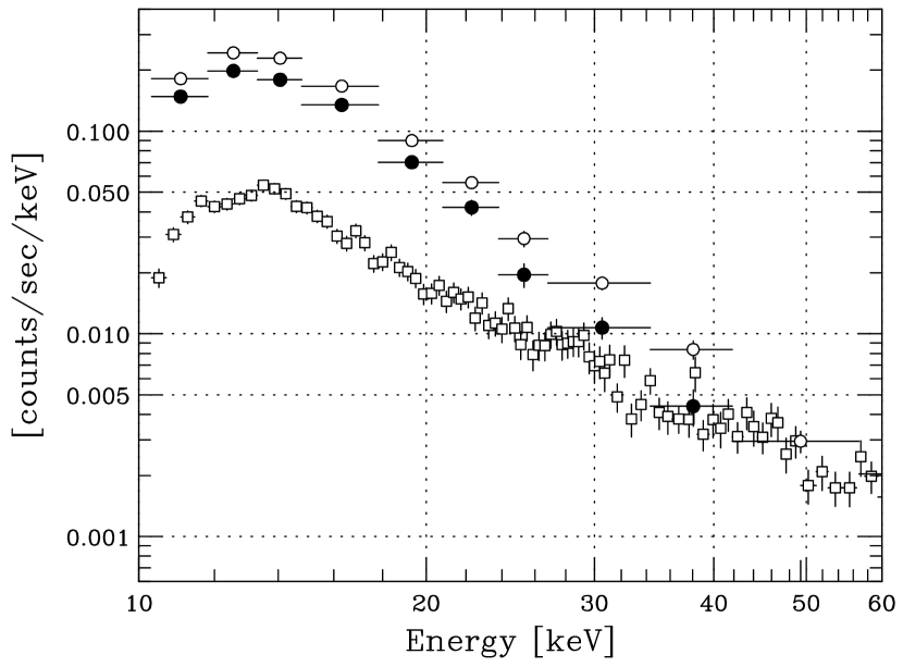
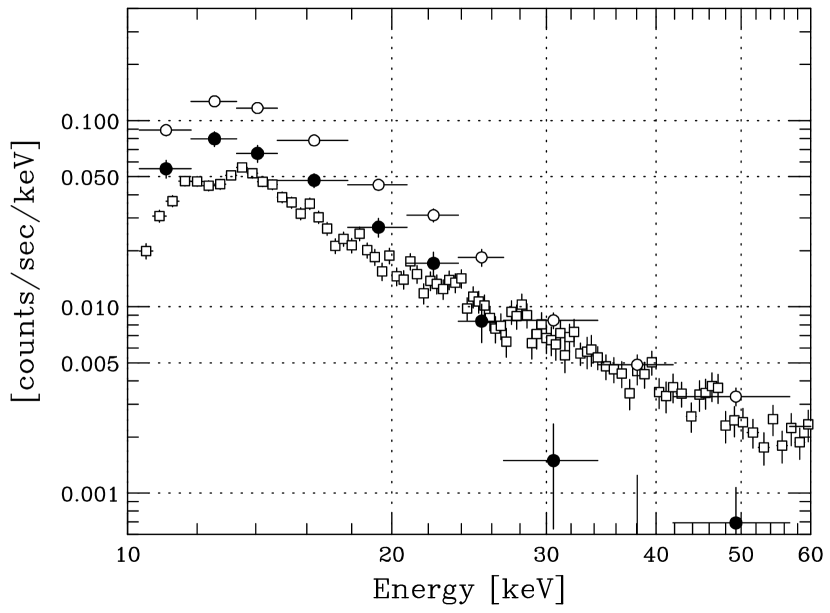
Figure 4.— The raw spectra of HXD/PIN at the brightest period (upper panel) and at the lowest period (lower panel). Only 750 sec accumulation time is used for the brightest period and 1.7 ksec for the lowest period. The open circles, open squares and filled circles show the raw data, background (NXB + CXB), and background-subtracted data, respectively.

In order to study the time evolution exhibited in the light curves more quantitatively, we divide the XIS and HXD data into 14 time intervals and perform spectral fitting to XIS+HXD spectra derived from each time interval. Raw HXD/PIN spectra during the highest and the lowest flux periods are shown in Figure 4. During the observation, the flux below 20 keV is always higher than that of the NXB. At the lowest flux period (lower panel of Figure 4), flux level is comparable to the NXB around 25 keV and about 30 % of the NXB level above 25 keV. Since the systematic error of the NXB is about 5 % (Fukazawa et al., 2009), which is six times less than the flux level measured at the lowest flux period, the results of present analysis are not affected by the systematic uncertainties of the NXB. In the following spectral analysis, the column density is fixed to the Galactic value: $N_{H}=0.0161\times 10^{22}~{}{\rm cm}^{-2}$ (Lockman & Savage, 1995) and the cross normalization between XIS and HXD/PIN is also fixed to 1.13 (Kokubun et al., 2007).

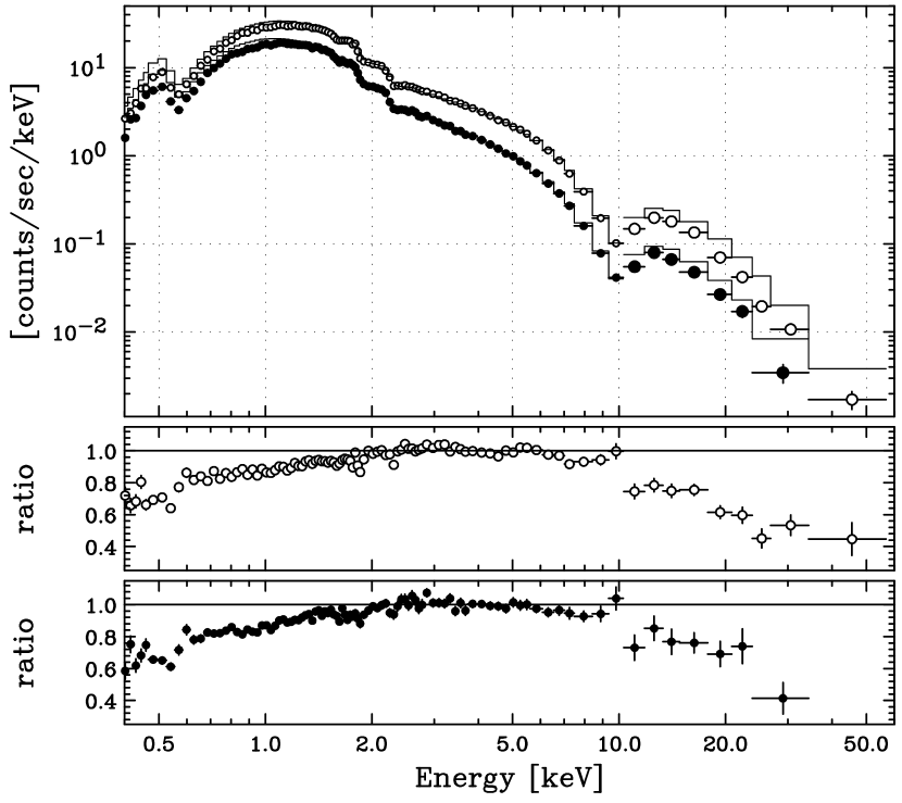
Figure 5.— XIS$+$PIN spectra in the energy range 0.4–60 keV are shown with the best-fit models obtained by fitting the XIS spectrum (2–5 keV) alone with power law model. The data points below/above 10 keV correspond to XIS and PIN data respectively. The lower panels show the ratio between the data points and the model values for the highest and the lowest periods.

Wide band spectrum obtained by Suzaku enables us to measure time-resolved behavior of the continuum spectrum, including even small deviations from a simple power law model. Firstly, in order to see how the spectra deviate from power law function, we restrict the fitting range to 2–5 keV. The results of fitting are shown in Figure 5, and as is clearly seen in the ratio, the spectra gradually curve downwards for both cases, meaning the power law index increases with increasing energy. Such a departure from a simple power law model appears to be a general feature of X-ray spectra of BL-Lac type blazars with the peak of the synchrotron component in the UV to soft X-ray band (see, e.g., Perlman et al., 2005). It is apparent that the spectrum changes with time, even in this restricted energy range: the spectral indices of power law model (2–5 keV) significantly change from 2.05$\pm$0.02 to 2.27$\pm$0.03, with the flux-index correlation in the sense where the soft X-ray spectra soften as the flux decrease. This is consistent with the results published so far (e.g., Takahashi et al., 1996). Clearly, sensitive Suzaku observations indicate spectral variability on short time scales (a few hour), and provide an opportunity to derive important constraints in the context of more physical “synchrotron model,” where the data are directly fitted to a particle spectrum radiating via the synchrotron process. This treatment is covered in the following sections.

4.3. Interpreting the X-ray Spectrum in the Context of Physical Synchrotron Model

We can obtain constraints on the physical parameters of the synchrotron emission, such as $B$ and $\gamma_{\rm max}$, via fitting the spectra with the recent numerical model (Tanaka et al., 2008). Hereafter we simply call this model “synchrotron model.” In the model, we assume an electron spectrum has a form of power law with exponential-type cutoff at the maximum energy $E_{\rm max}$ (= $\gamma_{\rm max}m_{e}c^{2}$), namely,

$$\frac{dN_{e}}{dE}=N_{e0}E^{-s}{\rm exp}\left[-\left(\frac{E}{E_{\rm max}}\right)^{\beta}\right].$$ (2)

Here, $s$ is the energy index of electron distribution, while $\beta$ and $N_{e0}$ (electrons cm^-3 eV^-1) determine the shape of high energy end of the population and the normalization, respectively. As described in Kataoka et al. (1999), we assume the spherical and uniform emitting region. The total power per unit frequency $P(\epsilon)$ can be written as

$$P_{\rm tot}(\epsilon)\propto\int F\left(\frac{\epsilon}{\epsilon_{c}}\right)\frac{dN_{e}}{dE}dE.$$ (3)

Here $\epsilon$ and $E$ parameters indicate the photon and electron energy, respectively, and the function $F(x)$ is defined as

$$F(x)\equiv x\int_{x}^{\infty}K_{5/3}(\xi)d\xi,$$ (4)

where $K_{5/3}(\xi)$ is the modified Bessel function of 5/3 order. When pitch angles are isotropic, the characteristic photon energy, $\epsilon_{c}$, is given as

$$\epsilon_{c}=5.43~{}\left(\frac{B}{0.10~{}{\rm G}}\right)\left(\frac{E}{1~{}{\rm TeV}}\right)^{2}~{}{\rm keV}.$$ (5)

This model has three free parameters; $s$, $\Pi\equiv E_{\rm max}{B}^{1/2}$  [GeV G^1/2] and the normalization of a spectrum. We note here that this synchrotron model is in fact based on the distribution of energies of radiating particles that is essentially a power law with an exponential (or hyper-exponential) cutoff. Such a distribution is similar to that which has been calculated to stochastic acceleration via the Fermi II process - such as, for instance, via scattering in magnetic turbulent regions in plasma (see, e.g., Stawarz & Petrosian, 2008).

In the case of emission from a jet, we need to consider the effect of relativistic beaming, since the fitted value of $\Pi$ ($\Pi_{\rm obs}$) is not given in the jet’s frame ($\Pi_{\rm jet}$), but instead $\Pi_{\rm obs}=\Pi_{\rm jet}\times\delta^{1/2}$. We adopt the Doppler (beaming) factor $\delta=10$: this value was directly measured by VLBI observations (e.g., Vermeulen & Cohen, 1994) which is consistent with the result obtained by simultaneous multi-band analysis from radio to $\gamma$-ray (Kubo et al., 1998). We note that more recent work by Lichti et al. (2008) which analyzes the big outburst followed by some weeks with respect to our Suzaku observation and suggests $\delta=15$ by modeling the SED. However, these differences are not the scope of our paper and will not affect our discussion.

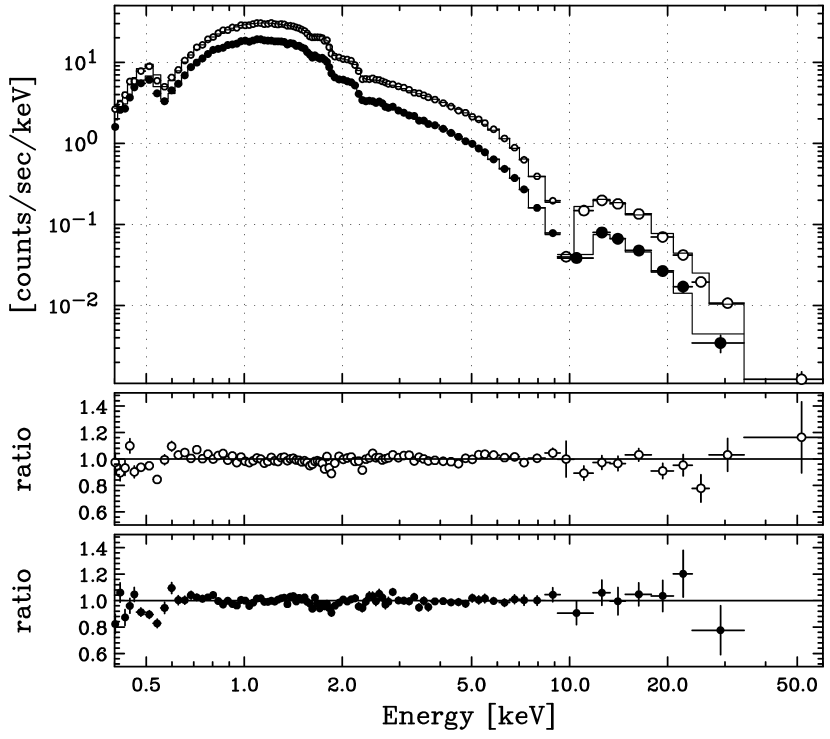
Figure 6.— The same as Figure 5 but fitting with simple synchrotron model in entire energy band 0.4–60 keV.

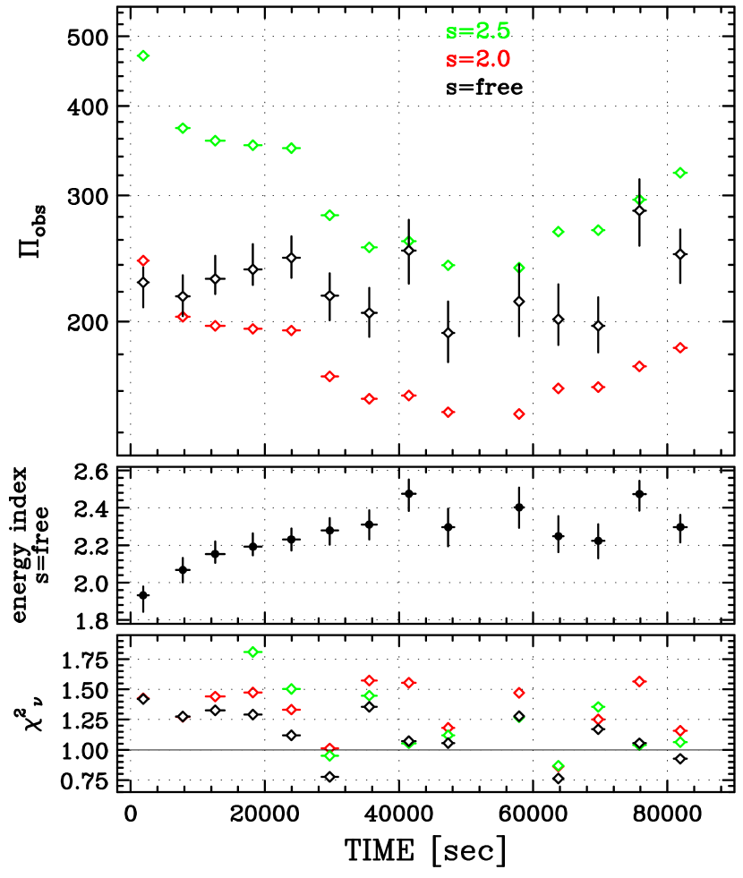
Figure 7.— The results of fitting time-resolved spectra with simple synchrotron model. The top panel represents the evolution of $\Pi_{\rm obs}$ values in units of GeV G^1/2 obtained by fitting each spectrum in the case of the energy index of electron spectrum fixed to $s=2.0$ (red), $s=2.5$ (green) and $s={\rm free}$ (black). The error bars include only statistical $1\sigma$ errors and those for green and red diamonds are too small to be seen. The middle panel shows the history of the energy index of electron spectrum in the case of $s={\rm free}$. In the bottom panel, we show the $\chi_{\nu}^{2}$ values corresponding to 59 and 60 d.o.f.

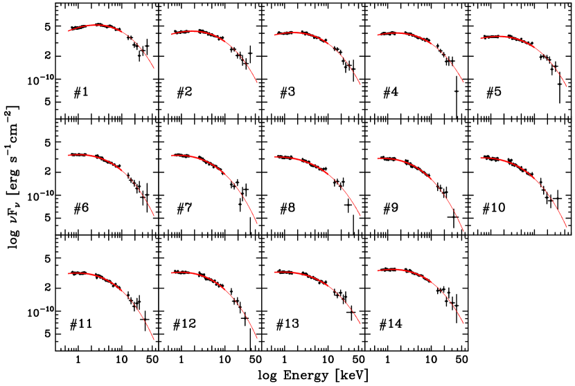
Figure 8.— SED for each good time interval fitted by “synchrotron“ model.

When we perform the spectral fitting for each data set with this model with $\beta$ fixed to unity, almost all the individual spectra are well fitted by this synchrotron model. In the fitting, we exclude the bandpass 1.5–2.5 keV and 8.0–10.0 keV because there remains some calibration uncertainties of the XIS detectors. Moreover, we fix the energy index of electron distribution ($s$) to be 2.0: then, the reduced chi-square ($\chi_{\nu}^{2}$) is ranging from 0.86 to 1.57 with 57 degrees of freedom (dof). In some time intervals, the $\chi_{\nu}^{2}$ values are substantially larger than in others and the model will be rejected. However, relatively large values of $\chi_{\nu}^{2}$ are partially caused by the insufficient calibration of the XIS/XRT rather than the inappropriate modeling of the spectra. Figure 6 shows the typical examples of the results for the highest- and the lowest-flux periods. For those, we obtain $\Pi_{\rm obs}$ = $243\pm 2$ ($\chi_{\nu}^{2}=1.42$ for 57 dof) and $149\pm 1$ ($\chi_{\nu}^{2}=1.18$ for 57 dof) [GeV G^1/2] for the highest and the lowest period, respectively.

We summarize the fitting results of each spectrum by the “synchrotron” model in Figure 7. The top panel of Figure 7 shows the evolution of $\Pi_{\rm obs}$ as a function of time, where the data points in red color correspond to the case of $s=2.0$. With $s=2.0$, the $\Pi_{\rm obs}=E_{\rm max}B^{1/2}\delta^{1/2}$ varies largely as the flux changes. In order to study how the energy index of electrons affects the results, we also fit those spectra with $s=2.5$, which is shown by the green markers in the Figure 7. The $\Pi_{\rm obs}$ values in the case of $s=2.5$ are significantly different (higher) from those in the case of $s=2.0$. In both cases, $\Pi_{\rm obs}$ parameters change by a factor of 2. On the other hand, when we treat $s$ as a free parameter, $\Pi_{\rm obs}$ does not change significantly, while $s$ increases from 1.95 to 2.55 in the decreasing phase. Statistically, $\chi_{\nu}^{2}$ for the case of $s$ as free is the lowest in any time intervals compared with in the case of fixed $s$ by only an additional degree of freedom, except for the first and the second time intervals. The interpretation of those results is discussed in § 5.1.

The spectra are fitted fairly well with the model based on synchrotron emission. In Figure 8, we plot the spectra in $\nu$–$\nu F_{\nu}$ space for all the data sets. All the spectra have convex shape. The shape of these spectra change significantly, and that is quite pronounced in the first interval (#1). In the first half of the observation, the flux decreases as the synchrotron peak frequency gradually shifts to lower band, that is, to $\sim 5$ keV at the highest period (# 1) and below 0.4 keV at the lowest period (# 9). On the other hand, in the second half, the synchrotron peak frequency does not seem to change apparently, as the flux increases.

Since X-ray spectra of blazars are often fitted to a spectral model involving a broken power law, for comparison, we attempted such a model. In all cases, the broken power law (involving three free parameters plus normalization, namely index before the break, after the break, and the break energy) returns a worse fit than the synchrotron model (where we used $s$ fixed at 2): for instance, for period # 1, $\chi_{\nu}^{2}$ is 1.42 for 57 dof for the “synchrotron” model while it is 2.28 for the broken power law; for period #2, the values are respectively 1.27 vs. 1.40: the broken power law model appears to have a break that is too sharp to fit the data. As it will become important in the discussion below, most relevant is the comparison of the two models for the period # 9: here, the values are respectively 1.18 vs. 1.90.

4.4. Spectral Analysis of the Steady and the Variable Components

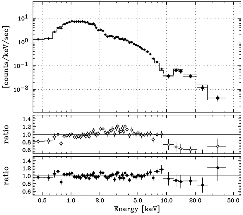
Figure 9.— Power law and broken power law fit for a subtracted spectrum. This is a case of second time interval (# 2) out of 14. The middle and bottom panels represent the ratio between data and model for simple power law and for broken power law model.

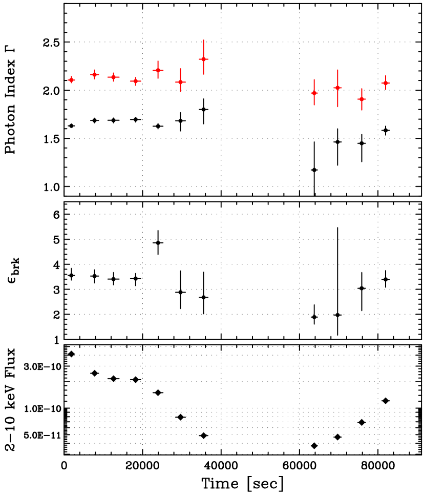
Figure 10.— Evolution of “variable” spectra. Top and middle panels show the history of the photon indices for lower (black; $\Gamma_{\rm lo}$) and higher (red; $\Gamma_{\rm hi}$) energy band and the break energy ($\epsilon_{\rm brk}$) in units of keV. We consider the “steady” component to correspond to the lowest-flux state (# 9). The vicinity of # 9, that is, # 8 and # 10 are excluded because of relatively poor statistics. Bottom panel shows that of the 2–10 keV flux in units of erg s^-1cm^-2.

Table 1 Fit results of the “variable” components with a broken power law function

#	$\Gamma_{\rm lo}$	$\epsilon_{\rm brk}$	$\Gamma_{\rm hi}$	2–10 keV flux	$\chi_{\nu}^{2}$ (dof)
1	$1.63^{+0.02}_{-0.02}$	$3.6^{+0.3}_{-0.2}$	$2.11^{+0.04}_{-0.03}$	$4.12\times 10^{-10}$	$1.25$ (54)
2	$1.69^{+0.02}_{-0.02}$	$3.5^{+0.2}_{-0.3}$	$2.16^{+0.05}_{-0.04}$	$2.49\times 10^{-10}$	$1.08$ (54)
3	$1.69^{+0.02}_{-0.03}$	$3.4^{+0.3}_{-0.2}$	$2.13^{+0.04}_{-0.04}$	$2.16\times 10^{-10}$	$0.87$ (54)
4	$1.70^{+0.02}_{-0.03}$	$3.4^{+0.2}_{-0.3}$	$2.09^{+0.04}_{-0.04}$	$2.10\times 10^{-10}$	$1.23$ (54)
5	$1.63^{+0.03}_{-0.03}$	$4.9^{+0.5}_{-0.5}$	$2.21^{+0.10}_{-0.08}$	$1.50\times 10^{-10}$	$0.97$ (27)
6	$1.68^{+0.09}_{-0.10}$	$2.9^{+0.8}_{-0.7}$	$2.08^{+0.14}_{-0.10}$	$7.90\times 10^{-11}$	$0.81$ (27)
7	$1.80^{+0.11}_{-0.15}$	$2.7^{+1.0}_{-0.7}$	$2.32^{+0.20}_{-0.16}$	$4.88\times 10^{-11}$	$1.17$ (27)
11	$1.17^{+0.29}_{-0.35}$	$1.9^{+0.5}_{-0.3}$	$1.97^{+0.14}_{-0.12}$	$3.75\times 10^{-11}$	$0.72$ (27)
12	$1.46^{+0.14}_{-0.24}$	$2.0^{+3.5}_{-0.8}$	$2.02^{+0.18}_{-0.20}$	$4.70\times 10^{-11}$	$1.14$ (27)
13	$1.45^{+0.09}_{-0.19}$	$3.0^{+0.6}_{-0.9}$	$1.91^{+0.11}_{-0.11}$	$6.91\times 10^{-11}$	$0.75$ (54)
14	$1.58^{+0.04}_{-0.05}$	$3.4^{+0.3}_{-0.3}$	$2.07^{+0.08}_{-0.07}$	$1.21\times 10^{-10}$	$0.80$ (54)

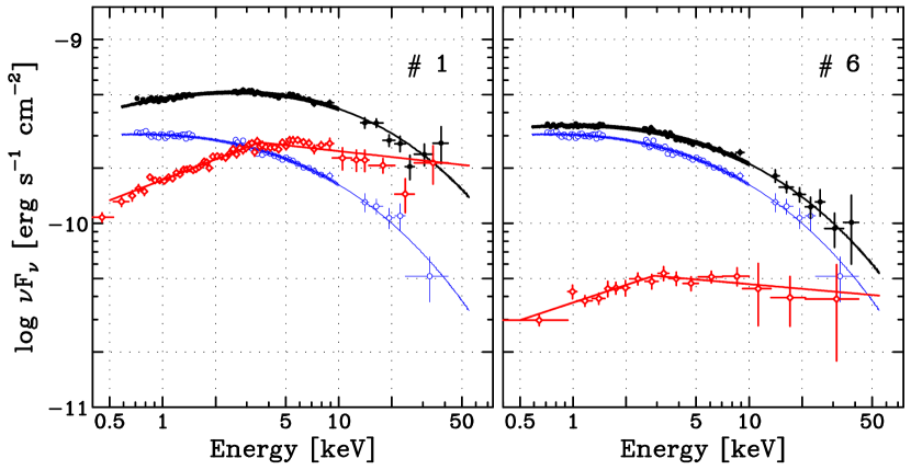
Figure 11.— Simultaneous plots of “variable” and “steady” components for the highest flux period (epoch # 1, left panel) and the end of decay period (epoch # 6, right panel). The red and black data set are for the “variable” components and the total (=“steady”+“variable”) spectra. The blue data set corresponds to the lowest-flux period and is common to two plots.

One possible approach towards the exploration of the spectral evolution during the observation is to separate the X-ray data into a “steady” and a “variable” components. In reality, “steady” means slowly-variable, variable on time scales much longer than typical X-ray observations lasting for one or several days, since historically the source flux does drop well below the level of our “steady” level. We associate the “variable” component with a newly injected electron distribution which drives the flare activity. We consider the “steady” component to correspond to the lowest state spectrum (# 9), which is illustrated in Figure 4 and well described by the synchrotron model in Figure 6, and the “variable” component to be the difference of individual spectra obtained at other epochs minus that of the lowest state spectrum.

In order to unveil the characteristics of “variable” component, we fit each of the subtracted spectra with simple power law model. The photon index of the subtracted spectrum is found to be harder, $\Gamma\sim 1.8$, but it also shows a large discrepancy between data and model and therefore is not well fitted by this model. Next we attempt a broken power law model and find that this model is acceptable for all the time intervals. An example of the fitting is shown in Figure 9 comparing with that of simple power law model, corresponding to the epoch # 2, and $\chi_{\nu}^{2}$ is significantly improved from 3.13 (56 dof) to 1.08 (54 dof). Subsequently, we fit all of the intervals with such a broken power law spectrum : Figure 10 shows the time history of parameters, that is, the photon index of low energy band ($\Gamma_{\rm lo}$) and of high energy band ($\Gamma_{\rm hi}$), and the break energy ($\epsilon_{\rm brk}$), which are summarized in Table 1. The vicinity of the epoch # 9 are excluded because the relatively large statistical errors of energy bins make it difficult to extract meaningful values. The 2–10 keV flux of the “variable” component decreases from $4.1\times 10^{-10}$ to $4.9\times 10^{-11}$ erg s^-1cm^-2 (and of course to zero for interval # 9, by construction) with the e-folding decaying time of $1.7\times 10^{4}$ sec, that is, less than 5 hours.

These plots lead to two important results : (1) the spectral shape of “variable” component does not vary across entire observation and only the normalization changes and (2) the photon indices $\Gamma_{\rm lo}$ and $\Gamma_{\rm hi}$ are about 1.6 and 2.1 respectively, that is, the differences between them are equal to about 0.5, with the break energy in photon space remaining relatively constant, at $\epsilon_{\rm brk}\simeq 3$ keV. All this has important implications which we discuss in § 5.2.

It is interesting to compare the lowest spectrum - that corresponding to the # 9 epoch - to the remaining spectra. This is essentially a comparison of the “variable” and “steady” components. In Figure 11, we plot both spectra at the same graph in the $\nu$–$\nu F_{\nu}$ space; there, we illustrate the highest flux period (# 1 minus # 9) and the end of decaying period (# 6 minus # 9) for the “variable” components. The spectral shapes of the “steady” and “variable” components are quite different, specifically the spectral indices of “variable” components, both lower and higher energy band, are harder than these of “steady” component. Perhaps the most striking is the fact that the spectral shapes of “variable” components do not vary significantly, and only the normalization changes.

5. Discussion

In the previous section, we performed detailed spectral analysis of TeV blazar Mrk 421 obtained by Suzaku in the period of the large flare in 2006 April 28–29 and found that there are two different interpretations for their variability. Below, we consider the physical scenarios that might correspond to the two phenomenological models above.

5.1. Spectral Variability due to the Change of $\Pi_{\rm obs}$

In § 4.3, we successfully fitted the evolution of the X-ray spectrum by the synchrotron model. In the case where the energy index of electron population is allowed to be free, $\Pi_{\rm obs}$ parameter does not change significantly throughout the observation and the change of electron energy index $s$ appears to be the factor responsible for the spectral change. The electron energy index itself is unlikely to vary significantly, so if the spectral evolution is due to the change of single electron population, the observed variability must be due to the change of $\Pi_{\rm obs}$.

Using equation (2.31) in Inoue & Takahara (1996), $\Pi_{\rm obs}$ can be written as

$$\Pi_{\rm obs}=B^{1/2}\delta^{1/2}\gamma_{\rm max}m_{e}c^{2}=v_{s}Bm_{e}c\left[\frac{9e\delta}{80(u_{B}+u_{\rm sync})\sigma_{\rm T}\xi}\right]^{1/2}$$ (6)

where $v_{s}$, $u_{B}$, $u_{\rm sync}$, $\sigma_{\rm T}$ and $\xi$ are the shock velocity in the observer’s frame, the energy density of magnetic field and synchrotron seed photons, Thomson cross section, and the so-called gyro-factor (the ratio of the mean free path for scattering with magnetic disturbances compared to the Larmor radius), respectively. This equation assumes that the maximum energy of electron distribution is determined by equating the radiative cooling time to the accelerating time. From this equation, the variability of $\Pi_{\rm obs}$ can be explained by changes of one or more parameters such as $v_{s}$, $B$ (thus also $u_{B}$), $u_{\rm sync}$, $\xi$, or $\delta$. The degeneracy between the parameters can be broken by comparing the temporal and spectral behavior of the X-ray time series against the TeV flux history. For instance, if the magnetic field $B$ is mainly responsible for the changes of $\Pi_{\rm obs}$, it would require for the ratio of the synchrotron luminosity to the inverse Compton luminosity, $L_{\rm sync}/L_{\rm IC}$, significantly change as a function of time. However, such multi-wavelength studies require simultaneous X-ray and TeV data, which are not currently available for this Suzaku observation.

5.2. Spectral Variability due to Superposition of Steady and Variable Components

As an alternative and preferred scenario to explain the variable behavior of Mrk 421, we introduce two separate electron populations, one is “steady” and the other is “variable” corresponding to the steady and variable componsnts of the X-ray spectra. There, a fresh electron distribution, distinct than the pre-existing one, is newly injected into the same (or a different) region of the jet and is responsible for the observed variable portion of source flux.

One of the important results in § 4.4 is that the photon indices $\Gamma_{\rm lo}$ and $\Gamma_{\rm hi}$ are measured to be $\sim 1.6$ and $\sim 2.1$ for “variable” components. Surprisingly, the result suggests that electrons form the power law distribution of energy index $\sim 2$, which is predicted from the standard shock acceleration theory for both non-relativistic and relativistic case (Blandford & Ostriker, 1978; Kirk et al., 2000) and then suffer from synchrotron cooling. As for the variability, we have shown that the spectral shape of “variable” components does not vary throughout the observation and the break energy appears to stay constant around $\epsilon_{\rm brk}\sim 3$ keV. While it is possible to adjust other parameters simultaneously to keep $\epsilon_{\rm brk}$ constant, this would require simultaneous changes of several parameters, amounting to “fine-tuning“ of parameters. The simplest interpretation of this observational result is that the variability of the X-ray flux is only due to the change of the injection rate of electrons, $N_{e0}$ in Eq. (2). Since the break energy in the synchrotron spectrum ($\epsilon_{\rm brk}$) is constant, $B$, $\delta$ and $\gamma_{\rm brk}$ are also expected to stay constant. With this, the synchrotron luminosity is proportional only to the energy density of the particles:

$$L_{\rm sync}\propto u_{e}u_{B}\delta^{4}\propto u_{e}\delta^{2}\gamma_{\rm brk}^{-4}\propto N_{e0}.$$ (7)

We thus decompose the X-ray spectrum of Mrk 421 into a “steady” component described as due to an exponentially cutoff power law distribution of electrons, and the “variable” component, well-described as a broken power law photon spectrum. Here we can make a suggestion of physical picture for these two components: the “variable” component is due to electrons efficiently accelerated in relatively small regions, such as localized shocks, via Fermi I process. In addition to that, a relatively “steady” component contributes as well: one possibility would be that the observed spectrum of this component is produced by shocks located at larger distance along the jet from the black hole. Such picture, invoking an internal shock scenario, was suggested by Tanihata et al. (2003). There, the resolved, rapid flares are due to collisions of pairs of shells at a characteristic distance $D_{\rm ch}$ from central engine, while those colliding at larger distance than $D_{\rm ch}$ make up the underlying, slowly variable component. Alternatively, the “steady” component might be associated with another process: the electrons escaping from the shock region into more extended volume are re-accelerated via Fermi II process on turbulence sites, as would be in the scenario described by several authors (Virtanen & Vainio, 2005; Katarzyński et al., 2006; Stawarz & Petrosian, 2008). This process operates in a larger volume, and thus the longer variability time scale. This scenario is particularly attractive as it is strongly supported by the spectral shapes and relative variability time scales of the two putative components. Specifically, the photon spectrum calculated for the diffuse acceleration process by Stawarz & Petrosian (2008) is similar to that derived via the synchrotron model, described and applied by us above.

With regard to the “variable” component, we infer an important implication of the fact that the observed break energy seems not to change throughout the observation. There, the break seen in the photon spectrum might be due to a competition between acceleration and cooling of relativistic electrons and expressed as

$$\gamma_{\rm brk}=\frac{3m_{e}c^{2}}{4(u_{\rm B}+u_{\rm sync})\sigma_{\rm T}R}$$ (8)

where $R$ is the size of emitting region (Inoue & Takahara, 1996). To be exact, $u_{\rm sync}$ in Eq.(8) is actually an increasing function of $N_{e0}$ via Eq. (7) and this implies $\epsilon_{\rm brk}$ should increase as the flux of “variable” component decreases. However, the fact that $\epsilon_{\rm brk}$ does not seem to change throughout the decaying phase of “variable” component suggests that the energy density of magnetic field is larger than that of soft seed photons ($u_{B}\gg u_{\rm sync}$) for “variable” components. This in turn suggests the synchrotron loss is dominant over the inverse Compton loss ($u_{B}/u_{\rm sync}=L_{\rm sync,var}/L_{\rm IC,var}\gg 1$).

6. Summary

We performed a detailed analysis of bright TeV blazar Mrk 421 data collected with Suzaku during the large flare in 2006 April 28–29. During the observation, the flux varied from $3.7\times 10^{-10}$ to $7.8\times 10^{-10}$ erg s^-1cm^-2. Thanks to the high sensitivity of Suzaku, we obtain the time-resolved spectrum of wide energy band 0.4–60 keV in intervals as short as $\sim$ 1 ksec.

Our detailed, time-resolved spectral analysis leads to two different scenarios describing the variability of Mrk 421. One is the conventional, one-component picture: in order to interpret the spectrum, we introduce the synchrotron model for the fitting function and find that the variability is due to the change of $\Pi_{\rm obs}$, the products of $B^{1/2}$, $\delta^{1/2}$ and $\gamma_{\rm max}m_{e}c^{2}$. The variability of $\Pi_{\rm obs}$ can be explained by changes of one or more of them. However, since we cannot break the degeneracy only this observation, simultaneous X-ray and TeV $\gamma$-ray observation are required. The other scenario invokes also a second, separate electron distribution that is responsible for the variability and which has energy index $s\sim 2$; this distribution is distinct than the one responsible for the steady component. Here, the rapidly variable component might be due to localized shock (Fermi I) acceleration, while the more steady component might be due to the superposition of shocks located at larger distance along the jet or due to a larger-scale, stochastic (Fermi II) acceleration on turbulence sites in the shocked plasma.

It is not possible to distinguish which scenario correctly describes the emission mechanism solely via this observation. However, the multi-component scenario provides a meaningful hint to disentangle the puzzle of the emission mechanism, such as the “orphan” flares and the very short time scale ($\sim$ minutes) of variability observed in TeV $\gamma$-ray band. In order to investigate the emission mechanism of TeV blazars further, simultaneous broad-band, high-sensitivity observations are needed, especially in X-ray and GeV/TeV $\gamma$-ray band facilitating a comparison of the “variable” components over the entire broad-band blazar spectra. Those show a promise towards a progress for understanding the acceleration mechanism in the relativistic jet. Such observations will be possible using Suzaku, Fermi GeV $\gamma$-ray telescope and advanced Cherenkov $\gamma$-ray telescopes.

References

- Angel & Stockman (1980) Angel, J. R. P., & Stockman, H. S. 1980, ARA&A, 18, 321
- Albert et al. (2007) Albert, J., et al. 2007, ApJ, 663, 125
- Aharonian et al. (2005) Aharonian, F., et al. 2005, A&A, 437, 95
- Aharonian et al. (2007) Aharonian, F., et al. 2007, ApJ, 664, L71
- Baixeras (2004) Baixeras, C. 2004, arXiv:astro-ph/0403180
- Blandford & Ostriker (1978) Blandford, R. D., & Ostriker, J. P. 1978, ApJ, 221, L29
- Błażejowski et al. (2005) Błażejowski, M., et al. 2005, ApJ, 630, 130
- Bradt et al. (1993) Bradt, H. V., Rothschild, R. E., & Swank, J. H. 1993, A&AS, 97, 355
- Fossati et al. (2008) Fossati, G., et al. 2008, ApJ, 677, 906
- Fukazawa et al. (2009) Fukazawa, Y., et al. 2009, PASJ, 61, 17
- Gaidos et al. (1996) Gaidos, J. A., et al. 1996, Nature, 383, 319
- Ghisellini & Tavecchio (2008) Ghisellini, G., & Tavecchio, F. 2008, MNRAS, 386, L28
- Gruber et al. (1999) Gruber, D. E., et al. 1999, ApJ, 520, 124
- Hinton (2004) Hinton, J. A. 2004, New Astronomy Review, 48, 331
- Inoue & Takahara (1996) Inoue, S., & Takahara, F. 1996, ApJ, 463, 555
- Ishisaki et al. (2007) Ishisaki, Y., et al. 2007, PASJ, 59, S113
- Kataoka et al. (1999) Kataoka, J., et al. 1999, ApJ, 514, 138
- Kataoka et al. (2000) Kataoka, J., et al. 2000, ApJ, 528, 243
- Katarzyński et al. (2006) Katarzyński, K., et al. 2006, A&A, 453, 47
- Kirk et al. (1998) Kirk, J. G., Rieger, F. M., & Mastichiadis, A. 1998, A&A, 333, 452
- Kirk et al. (2000) Kirk, J. G., et al. 2000, ApJ, 542, 235
- Kokubun et al. (2007) Kokubun, M., et al. 2007, PASJ, 59, S53
- Koyama et al. (2007) Koyama, K., et al. 2007, PASJ, 59, 23
- Krawczynski et al. (2004) Krawczynski, H., et al. 2004, ApJ, 601, 151
- Kubo et al. (1998) Kubo, H., et al. 1998, ApJ, 504, 693
- Lichti et al. (2008) Lichti, G. G., et al. 2008, A&A, 486, 721
- Lockman & Savage (1995) Lockman, F. J., & Savage, B. D. 1995, ApJS, 97, 1
- Mitsuda et al. (2007) Mitsuda, K., et al. 2007, PASJ, 59, S1
- Perlman et al. (2005) Perlman, E. S., et al. 2005, ApJ, 625, 727
- Punch et al. (1992) Punch, M., et al. 1992, Nature, 358, 477
- Rebillot et al. (2006) Rebillot, P. F., et al. 2006, ApJ, 641, 740
- Serlemitsos et al. (2007) Serlemitsos, P.J., et al. 2007, PASJ, 59, S9
- Stawarz & Petrosian (2008) Stawarz, Ł., & Petrosian, V. 2008, ApJ, 681, 1725
- Takahashi et al. (1996) Takahashi, T., et al. 1996, ApJ, 470, L89
- Takahashi et al. (2000) Takahashi, T., et al. 2000, ApJ, 542, L105
- Takahashi et al. (2007) Takahashi, T., et al. 2007, PASJ, 59, S35
- Tanaka et al. (2008) Tanaka, T., et al. 2008, ApJ, 685, 988
- Tanihata et al. (2003) Tanihata, C., et al. 2003, ApJ, 584, 153
- Tanihata et al. (2004) Tanihata, C., et al. 2004, ApJ, 601, 759
- Tavecchio et al. (1998) Tavecchio, F., Maraschi, L., & Ghisellini, G. 1998, ApJ, 509, 608
- Tosti et al. (1998) Tosti, G., et al. 1998, A&A, 339, 41
- Ulrich et al. (1997) Ulrich, M.-H., Maraschi, L., & Urry, C. M. 1997, ARA&A, 35, 445
- Urry & Padovani (1995) Urry, C. M. & Padovani, P. 1995, PASP, 107, 803
- Vermeulen & Cohen (1994) Vermeulen, R. C., & Cohen, M. H. 1994, ApJ, 430, 467
- Virtanen & Vainio (2005) Virtanen, J. J. P., & Vainio, R. 2005, ApJ, 621, 313
- Wagner et al. (2008) Wagner, R. M. et al. 2008, MNRAS, 385, 119
- Weekes et al. (2002) Weekes, T. C., et al. 2002, Astroparticle Physics, 17, 221