Abstract

We present in this work a generalization of the solution of Gorenstein and Yang to the inconsistency problem of thermodynamics for systems of quasi-particles whose masses depend on both the temperature and the chemical potential. We work out several solutions for an interacting system of quarks and gluons and show that there is only one type of solution that reproduce both perturbative and lattice QCD.

PACS: 12.38.Mh, 25.75.Nq
Keywords: Quark-Gluon Plasma, Quasi-Particle.

1 Introduction

In the past two decades, strongly coupled matter under extreme conditions has been object of intensive study, as it must describe from the core of some neutron stars to important features of the early universe and heavy ion collisions experiments (see e.g. [1, 2]). It is the understanding that hadrons are composed by asymptotically free particles that led to the idea that at sufficiently high temperature $T$, and/or quark chemical potential $\mu$, the hadronic matter should be described by quarks and gluons degrees of freedom [3], the quark-gluon plasma (QGP). Current lattice calculations strongly suggests that this phase transition actually happens, in the case of a vanishing chemical potential, at a temperature around $T_{c}\simeq 190$MeV [4]. The search for a phase transition in the case of a non-vanishing quark chemical potential has recently advanced, as a result of new techniques for lattice calculations [5, 6, 7].

Results from ultra-relativistic heavy ion collisions at RHIC [8, 9, 10, 11], on the other hand, indicate that the QGP has already been produced, and that hydrodynamics is capable to describe the experimental data [12]. The basic input for hydrodynamics is the equation of state EoS, which must cover both the hadronic and the QGP sectors. The matter created in the heavy ion collisions has high $T$ and small $\mu$, therefore the study of the EoS at these conditions is of extreme importance for the hydrodynamics approach. The EoS of the hadronic phase is currently described by the hadronic resonance gas model [13], with a good agreement to lattice data [5, 14]. For the deconfined phase, one needs an EoS in terms of quark-gluon degrees of freedom. QCD at finite $T$ and $\mu$ is, in principle, the theoretical tool to compute the thermodynamics functions in this new phase. However, strict perturbation theory, which have been pushed to $g^{6}\ln(1/g)$ [15], is reasonable only for extremely high temperatures; at temperatures near $T_{c}$ it seems not to be applicable, and alternative treatments appear to be necessary. Moreover, the perturbative series seems to be weakly convergent [15, 16, 17]. Specifically, it is expected that when $T\gg T_{c}$, the plasma behaves like an ideal gas of quarks and gluons, but the perturbative series converges at a slow pace towards this expectation. A way to circumvent this problem is through the reorganization of the perturbative series. For instance, there are attempts to reorganize the series using the Hard-Thermal-Loop (HTL) effective action [18], in the form of so-called HTL perturbation theory [19, 20], and also attempts based on the 2-loop $\Phi$-derivable approximation [21, 22]. The latter approach assumes a massive quasi-particle formalism [23, 24].

Concomitantly, phenomenological models based on quasi-particles have had success in describing the lattice data [23, 24, 25, 26, 27, 28, 29, 30], over a wide range of temperatures (and at $\mu=0$), in addition to being compatible with the fluid-like behavior found at RHIC [31]. More recently, a quasi-particle model for the quark-gluon plasma (qQGP) for a non-vanishing $\mu$ has also been worked out [32, 33, 34], with a satisfactory description of the lattice data. Besides the quasi-particle approach, there are other treatments to describe lattice data near the transition region as, for instance, the Polyakov loop enhanced Nambu-Jona-Lasinio (PNJL) model [35, 36], which is able to fit lattice data quite well, even when $\mu\neq 0$.

The quasi-particle model of the quark-gluon plasma is a phenomenological model that assumes non-interacting massive quasi-particles which, with the aid of few parameters, like the thermal masses, is able to fit lattice QCD data over a wide range of temperatures [25, 26, 27]: Not only at extremely high temperatures, as in strict perturbation theory, or when $T>20T_{c}$, as in the HTL perturbation theory, but also near $T_{c}$. Indeed, quasi-particle models intend to describe deconfined matter from $T_{c}$ up to $T\rightarrow\infty$, although from the point of view of linking the QGP with hydrodynamics calculations, the reproduction of lattice data near $T_{C}$ is somewhat more important.

The problem with the quasi-particle models is that the thermodynamics relations calculated from them are not consistent [37]. Its origin is in the use of Standard Statistical Mechanics (SSM) [38] with dispersion relations for quasi-particles that resembles the dispersion relations for free particles. Contrary to the case of particles, quasi-particles have masses that are dependent on $T$ and/or $\mu$. The first work to systematically study the consistency problem, and solve it for finite $T$ but zero chemical potential, was the one by Gorenstein and Yang [37]. In their approach, it is built an effective Hamiltonian which is composed of a part representing an ideal gas and a part representing contributions from the vacuum. This extra vacuum term leads to a modification in the pressure and in the internal energy of the system, but keeps the entropy and the number density untouched. In this way, a consistent thermodynamics for quasi-particles is obtained. Most of the works in the literature are based on this approach [39]. More recently, several authors have also turned their attention to the thermodynamics consistency of quasi-particle systems. In [40], the authors build an effective Hamiltonian, $H_{eff}$, as before but require that the average of $\partial H_{eff}/\partial\mu$ and $\partial H_{eff}/\partial T$ are zero. As a result, they get expressions for the thermodynamics functions of the same kind found in [37]. On the other hand, in [41], the particle mass is taken as an independent variable. In this case, it is also found a set of consistent thermodynamics relations. Other possibility is presented in [28], where instead of keeping the entropy unchanged, as Gorenstein and Yang, the internal energy preserves its SSM definition, in a way that the consistency of the thermodynamics relations is also achieved. Finally, a set of solutions for the thermodynamics of quasi-particles at $\mu=0$ was presented in [30]. There it is shown that the solutions of references [28, 37] are particular solutions of a general formulation. The next natural step is to extend this formulation to the case of finite $\mu$.

In this work, a framework for the thermodynamics of a system composed of quasi-particles whose masses are $T$ and $\mu$ dependent is developed, generalizing [30]. At first sight, a system composed of a mixture of fermions and bosons should follow the law of Dalton for gas mixtures. This law states that the pressure exerted by a mixture of gases is equal to the sum of the partial pressures of all the components present in the mixture. This statement holds exactly for ideal gases. For real gases, however, the equality is approximated. As the quasi-particle approach is built on the ideal gas model, one would expect that the pressure for the whole system, i.e. for quarks and gluons, were the sum of the fermionic and bosonic parts, separately. In reality, this should not be true in the qQGP because the underlining theory is that of an interacting system. It makes no sense to fix the number of gluons $n_{g}=\partial P_{g}/\partial\mu=0$, since no energy is expended for their creation ($\mu_{g}=0$). On the other hand if the pressure is computed from Ref. [30], with a suitable Debye mass, $m_{D}\equiv m_{D}(T,\mu)$, and including fermions, it can be seen from the thermodynamics relations that the number of gluons will be different from zero $n_{g}=\partial P_{g}(m_{D})/\partial\mu\neq 0$. Therefore, the law of Dalton fails here, implying that it is necessary to develop the theory for the whole system, and not for each part independently.

This article is organized as follows. In Sec. II, the general formalism for a consistent thermodynamics of quasi-particles in the grand canonical ensemble is presented. In sections III and IV, particular solutions for this thermodynamics are computed, and in section V a comparison with perturbative QCD is made. In section VI, the comparison is with lattice QCD and, finally, the conclusions are presented in section VII.

2 The Formalism

In the quasi-particle approach for the quark-gluon plasma, the system is described by an effective Hamiltonian with mass terms that are dependent on $T$ and/or $\mu$ [23, 24, 30, 33]. As widely known, early attempts to implement this idea run in a serious problem: an inconsistency in the thermodynamics relations. As shown by Gorenstein and Yang [37], it is not enough to use the Hamiltonian of an ideal gas with the mass $m$ replaced by the effective mass $m(T,\mu)$. An extra term, $B$, has to be added to the original Hamiltonian: $H\rightarrow H+\eta B$, where $\eta B$ is regarded as the zero point energy of the system. The extra term modifies the usual thermodynamics functions, healing the thermodynamics inconsistency of the system. Thus, the most general form for the thermodynamics functions can be written as:

$$\Phi(V,T,\mu,m_{f}^{2},m_{b}^{2}) = \Phi_{f}(V,T,\mu,m_{f}^{2})+\Phi_{b}(V,T,\mu,m_{b}^{2})+{\alpha}B(V,m_{f}^{2},m_{b}^{2}),$$ (1)

$$U(V,T,\mu,m_{f}^{2},m_{b}^{2}) = U_{f}(V,T,\mu,m_{f}^{2})+U_{b}(V,T,\mu,m_{b}^{2})+\eta B(V,m_{f}^{2},m_{b}^{2}),$$ (2)

$$S(V,T,\mu,m_{f}^{2},m_{b}^{2}) = S_{f}(V,T,\mu,m_{f}^{2})+S_{b}(V,T,\mu,m_{b}^{2})-\frac{\gamma}{T}B(V,m_{f}^{2},m_{b}^{2}),$$ (3)

$$N(V,T,\mu,m_{f}^{2},m_{b}^{2}) = N_{\{f\}}(V,T,\mu,m_{f}^{2})-\frac{\lambda}{\mu}B(V,m_{f}^{2},m_{b}^{2}),$$ (4)

where $\Phi=-PV$ is the grand potential, $U$ is the internal energy, $S$ is the entropy, and $N$ is the average net quark number. The subscripts $f$ and $b$ denote fermions and bosons, respectively. The functions $m_{f}^{2}=m_{f}^{2}(T,\mu)$ and $m_{b}^{2}=m_{b}^{2}(T,\mu)$ are the dynamical masses acquired by fermions and bosons. The constants $\alpha$, $\eta$, $\gamma$ and $\lambda$ are arbitraries, but constrained by $\alpha=\eta+\gamma+\lambda$, to guarantee the consistency of the fourth thermodynamic relation in Eqs. (5) below. This condition is just the extension of the constraint obtained in Ref. [30]. The $T$ and $\mu$ dependency of $B(V,m_{f}^{2},m_{b}^{2})$ is assumed to be through the masses only. The extra term $B(V,m_{f}^{2},m_{b}^{2})$ must be such that the thermodynamics relations

$$P=-\left(\frac{{\partial}\Phi}{{\partial}V}\right)_{T,\mu},\hskip 11.38092ptS=-\left(\frac{\partial\Phi}{{\partial}T}\right)_{V,\mu},\hskip 11.38092ptN=-\left(\frac{\partial\Phi}{\partial\mu}\right)_{T,V},\hskip 11.38092ptU=\Phi+TS+{\mu}N.$$ (5)

are valid. Substituting the Eqs. (1), (2), (3) and (4) in Eqs. (5), one finds the following pair of differential equations:

$$\gamma{B}=T\alpha\frac{\partial{B}}{\partial{T}}+T\sum_{i=b,f}\Bigg{\langle}\frac{\partial{H_{i}}}{\partial{T}}\Bigg{\rangle},\hskip 28.45274pt\lambda{B}=\mu\alpha\frac{\partial{B}}{\partial\mu}+\mu\sum_{i=b,f}\Bigg{\langle}\frac{{\partial}H_{i}}{\partial\mu}\Bigg{\rangle},$$ (6)

Using the connection between SSM and thermodynamics, $\Phi_{i}=-T\ln Z_{i}$, where $Z_{i}$ is the grand partition function with Hamiltonian $H_{i}$, one can deduce the following equalities: $\langle\frac{\partial{H_{i}}}{\partial{T}}\rangle=\frac{{\partial}m^{2}_{i}}{{\partial}T}(\frac{\partial\Phi_{i}}{\partial{m^{2}_{i}}})_{T,V,\mu}$ and $\langle\frac{\partial{H_{i}}}{\partial{\mu}}\rangle=\frac{{\partial}m^{2}_{i}}{{\partial}\mu}(\frac{\partial\Phi_{i}}{\partial{m^{2}_{i}}})_{T,V,\mu}$. Using these expressions, and assuming $\alpha\neq 0$, one concludes that the two equations in (6) are the same. They are rewritten as:

$$\frac{\partial}{\partial{m^{2}_{i}}}(BT^{-\frac{\gamma}{\alpha}}\mu^{-\frac{\lambda}{\alpha}})=-\frac{T^{-\frac{\gamma}{\alpha}}\mu^{-\frac{\lambda}{\alpha}}}{\alpha}\Bigg{\langle}\frac{\partial{H_{i}}}{\partial{m^{2}_{i}}}\Bigg{\rangle}\hskip 28.45274pt\alpha\neq 0,\hskip 28.45274pti=b,f.$$ (7)

For $\alpha=0$, the limit $\alpha\rightarrow 0$ in Eqs. (6) has to be taken with care. One obvious point is that the two equations for $B$ in (6) give different results if one simply sets $\alpha=0$. When the grand potential has no extra term, the average number of particles and the entropy must have extra terms, i.e. if $\alpha=0$ then $\gamma$ and $\lambda$ must be different from zero. If such condition is not fulfilled than the thermodynamics functions will not be consistent. This conclusion is based on the fact that the entropy and the average number of particles are obtained from the grand potential by Eqs. (5). Therefore the previous redefined thermodynamics functions are not valid when $\alpha=0$, and the modified thermodynamics functions must have the following form:

$$\Phi=\Phi_{b}+\Phi_{f},S=S_{b}+S_{f}-\gamma\frac{B_{S}}{T},N=N_{\{f\}}-\lambda\frac{B_{N}}{\mu},U=U_{b}+U_{f}-\lambda{B_{N}}-\gamma{B_{S}},$$ (8)

where $B_{S}$ and $B_{N}$ are

$$B_{S}=\frac{T}{\gamma}\sum_{i=b,f}\Bigg{\langle}\frac{\partial{H_{i}}}{\partial{T}}\Bigg{\rangle},\hskip 14.22636ptB_{N}=\frac{\mu}{\lambda}\sum_{i=b,f}\Bigg{\langle}\frac{\partial{H_{i}}}{\partial{\mu}}\Bigg{\rangle}\hskip 65.44142pt\alpha=0.$$ (9)

The solutions for $B$ given by Eq. (9) are inversely proportional to $\lambda$ and $\gamma$, respectively. Thus, Eqs. (8) are independent of $\gamma$ and $\lambda$, differently from the $\alpha\neq 0$ case.

As in the canonical case [30], the physical meaning of $B(V,T,\mu)$ can be extracted from quantum statistical mechanics. Using the quantum form for the internal energy, one has

$$U=\langle\sum_{b,f}\hat{H}\rangle+{\eta}B=Tr[\hat{\rho}(\sum_{b,f}\hat{H}+\eta\hat{B})],$$ (10)

where $\hat{\rho}=e^{-\beta\hat{H}+\beta\mu\hat{N}}/Z$ is the ensemble density operator, $\hat{H}$ is the Hamiltonian operator, $\hat{N}$ is the number operator, and $\hat{B}\equiv B\textbf{1}$ is the extra term with the unity operator. Note that when a term independent of $q$ and $p$, but dependent on $T/\mu$, is added to the Hamiltonian, the density operator for this modified Hamiltonian is exactly the same as that obtained using the original Hamiltonian, i.e. the density operator is defined up to a $T/\mu$ function in the Hamiltonian. Thus, one can add $\hat{B}$ to $\hat{H}$ in $\hat{\rho}$ without inducing any change in Eq. (10). Using this property, it is seen that Eq. (10) has the same definition as in the $SSM$ case: $U$ is given by the average value of the system Hamiltonian. Therefore, the complete Hamiltonian, particles plus vacuum, which must be used in the quasi-particle picture, is $\hat{H}_{T}=\sum\hat{H}+\hat{E}_{0}$, with $\hat{E}_{0}=\eta\hat{B}$ the zero point energy. The standard procedure of discarding the zero point energy can not be used here, since it results in uncompleted thermodynamics functions, causing an inconsistency.

For the average number of particles, the same manipulation (as for the internal energy) can be applied to the $N$ quantum expression, where instead of adding a $T/\mu$ function to the Hamiltonian, one adds it to the $\hat{N}$ operator. Thus, ${N}$ follows the same definition as in the $SSM$: ${N}$ is given by the mean value of the total number operator, where the total number operator is $\hat{N}_{T}=\hat{N}+\hat{N}_{0}$, with $\hat{N}_{0}=-\frac{\lambda}{\mu}\hat{B}$. The extra term $-\lambda\hat{B}/\mu$ represents the number of particles associated with the zero point energy, which means that one can regard the zero point energy of the quasi-particle scenario, multiplied by suitable constants, as a mechanism to add or subtract particles from the system.

These redefinitions imply the following thermodynamics functions:

$$S=-\langle\ln\hat{\rho}\rangle-\gamma\frac{B}{T},\hskip 11.38092pt\Phi=-T{\ln}Z_{T}+\gamma{B},\hskip 11.38092ptN=\langle\hat{N}_{T}\rangle,\hskip 11.38092ptU=\langle\hat{H}_{T}\rangle.$$ (11)

where $Z_{T}$ is the partition function with $\hat{H}_{T}$ and $\hat{N}_{T}$. Note that for $\gamma=0$, the statistical mechanics definitions for the entropy, the grand potential, the number of particles and the internal energy are the usual ones.

The interpretation for $B$ in the $\alpha=0$ case follows closely that of the $\alpha\neq 0$ case. Using again the quantum version of Eq. (8), the internal energy can be written as

$$U=U_{b}+U_{f}-\lambda{B_{N}}-\gamma{B_{S}}=\textrm{Tr}[\hat{\rho}(\sum_{i=b,f}\hat{H_{i}}-\lambda\hat{B}_{N}-\gamma\hat{B}_{S})],$$ (12)

where $\hat{B}_{j}\equiv B_{j}\textbf{1}$ is the operator for $j=N,S$. As before, $\hat{H}_{T}=\sum\hat{H}+\hat{E}_{0}$, where $\hat{E}_{0}=-\lambda\hat{B}_{N}-\gamma\hat{B}_{S}$ is the zero point energy, dependent on $T$ and $\mu$ dependent. In the quantum statistical mechanics picture, the self-consistent definition for the number of particles is

$$N=\langle\hat{N}\rangle-\frac{\lambda}{\mu}B_{N}=\textrm{Tr}\left[\hat{\rho}\left(\hat{N}-\frac{\lambda}{\mu}\hat{B}_{N}\right)\right].$$ (13)

Applying the same arguments as before, the total number of particles operator is $\hat{N}_{T}=\hat{N}+\hat{N}_{0}$, with $\hat{N}_{0}=-\frac{\lambda}{\mu}\hat{B}_{N}$ the number of particles associated with the zero point energy. Finally, the quantum statistical mechanics relations are written as a function of the total Hamiltonian

$$\Phi=-T{\ln}Z_{T}+{\gamma}B_{S},\hskip 8.5359ptS=-\langle\ln\hat{\rho}\rangle-\gamma\frac{B_{S}}{T},\hskip 8.5359ptN=\langle\hat{N}_{T}\rangle,\hskip 8.5359ptU=\langle\hat{H}_{T}\rangle.$$ (14)

To conclude this section, the solutions for both $\alpha\neq 0$ and $\alpha=0$ cases are summarized in the following table:

3 Thermodynamics Functions for $\alpha\neq 0$

To investigate the possible solutions for the thermodynamics of the system, one needs an expression for the extra term $B$. From Eq. (7), it is written as:

$${\alpha}B=B_{0}\mu^{\frac{\lambda}{\alpha}}T^{\frac{\gamma}{\alpha}}-\mu^{\frac{\lambda}{\alpha}}T^{\frac{\gamma}{\alpha}}\sum_{i=b,f}{\int}dm^{2}_{i}\Bigg{\langle}\frac{\partial{H_{i}}}{{\partial}m_{i}^{2}}\Bigg{\rangle}\mu^{-\frac{\lambda}{\alpha}}T^{-\frac{\gamma}{\alpha}},$$

or simply

$${\alpha}B=B_{0}\mu^{\frac{\lambda}{\alpha}}T^{\frac{\gamma}{\alpha}}-\mu^{\frac{\lambda}{\alpha}}T^{\frac{\gamma}{\alpha}}\sum_{i=b,f}\left[{\int}d\mu\Bigg{\langle}\frac{\partial{H_{i}}}{{\partial}\mu}\Bigg{\rangle}\mu^{-\frac{\lambda}{\alpha}}T^{-\frac{\gamma}{\alpha}}+{\int}dT\Bigg{\langle}\frac{\partial{H_{i}}}{{\partial}T}\Bigg{\rangle}\mu^{-\frac{\lambda}{\alpha}}T^{-\frac{\gamma}{\alpha}}\right].$$ (15)

As the approach developed here is completely general, particular choices for the constants $\alpha$, $\gamma$, $\lambda$, and $\eta$, should reproduce known results in the literature, as for instance the equations obtained by Gorenstein-Yang [37], and the ones obtained by Bannur [33].

3.1 The Solution of Gorenstein-Yang

In Ref. [37], the thermodynamics of a system whose masses depend on $T/\mu$ was studied through two conditions: (i) the thermodynamics functions are defined as in the standard Statistical Mechanics, and (ii) the pressure is minimized with respect to the phenomenological parameters. In the general solution presented here, the condition $\gamma=0$ guarantees (i), implying that the vacuum does not contribute to the total entropy of the system. The corresponding thermodynamics functions are then given by:

$$S = -\sum_{i=b,f}\langle\ln\hat{\rho_{i}}\rangle$$

$$\Phi = -\sum_{i=b,f}\left(T{\ln}Z_{i}+\mu^{\frac{\lambda}{\alpha}}{\int}d\mu\Bigg{\langle}\frac{\partial{H_{i}}}{\partial\mu}\Bigg{\rangle}\mu^{-\frac{\lambda}{\alpha}}+\int{dT}\Bigg{\langle}\frac{\partial H_{i}}{\partial T}\Bigg{\rangle}\right)+{\alpha}B_{0}\mu^{\frac{\lambda}{\alpha}}$$

$$N = \langle\hat{N}\rangle+\frac{\lambda}{\alpha}\mu^{-1}\sum_{i=b,f}\left(\int{dT}\Bigg{\langle}\frac{\partial{H_{i}}}{\partial{T}}\Bigg{\rangle}+\mu^{\frac{\lambda}{\alpha}}\int{d}\mu\Bigg{\langle}\frac{\partial{H_{i}}}{\partial\mu}\Bigg{\rangle}\mu^{-\frac{\lambda}{\alpha}}\right)-B_{0}\lambda\mu^{\frac{\lambda}{\alpha}-1}$$

$$U = \sum_{i=b,f}\left[\langle\hat{H_{i}}\rangle-\frac{\eta}{\alpha}\left(\mu^{\frac{\lambda}{\alpha}}\int{d}\mu\Bigg{\langle}\frac{\partial{H_{i}}}{\partial\mu}\Bigg{\rangle}\mu^{-\frac{\lambda}{\alpha}}+\int{dT}\Bigg{\langle}\frac{\partial{H_{i}}}{\partial{T}}\Bigg{\rangle}\right)\right]+{\eta}B_{0}\mu^{\frac{\lambda}{\alpha}}.$$ (16)

The solutions with $\gamma=0$ will be classified as of Gorenstein-Yang type of solution. They can be divided into two different branches.

3.1.1 The Original Solution

This is the most used solution, which satisfies both conditions (i) and (ii), and was used in several studies of QGP by quasi-particle model, as for instance in Refs. [23, 24, 25, 26, 27]. In this approach, neither the entropy nor the average number of particles are modified by any additional term coming from the vacuum. This solution is obtained by setting $\gamma=\lambda=0$, and $\alpha=\eta$. The thermodynamics functions are then reduced to:

$$S = -\sum_{i=b,f}\langle\ln\hat{\rho_{i}}\rangle$$

$$N = \langle\hat{N}\rangle$$

$$\Phi = -\sum_{i=b,f}\left(T{\ln}Z_{i}+{\int}d\mu\Bigg{\langle}\frac{\partial{H_{i}}}{\partial\mu}\Bigg{\rangle}+\int{dT}\Bigg{\langle}\frac{\partial H_{i}}{\partial T}\Bigg{\rangle}\right)+B_{0}$$

$$U = \sum_{i=b,f}\left[\langle\hat{H_{i}}\rangle-\mu^{\frac{\lambda}{\alpha}}\int{d}\mu\Bigg{\langle}\frac{\partial{H_{i}}}{\partial\mu}\Bigg{\rangle}\mu^{-\frac{\lambda}{\alpha}}-\int{dT}\Bigg{\langle}\frac{\partial{H_{i}}}{\partial{T}}\Bigg{\rangle}\right]+B_{0}.$$ (17)

As this solution is well know and has been largely studied, we will not provide here further details of its features, which can be found in Ref. [37]. It will be referred from now on as GY1.

3.1.2 The Modified Solution

A second solution of the type Gorenstein-Yang, is the one where $\alpha=\lambda$ and $\gamma=\eta=0$, meaning that both the entropy and the internal energy retain their original forms, while the other 2 thermodynamics functions are modified. Including bosons and fermions, the thermodynamics functions are now written as:

$$S = -\sum_{i=b,f}\langle\ln\hat{\rho_{i}}\rangle$$

$$U = \sum_{i=b,f}\langle\hat{H_{i}}\rangle$$

$$\Phi = -\sum_{i=b,f}\left(T{\ln}Z_{i}+\mu{\int}d\mu\Bigg{\langle}\frac{\partial{H_{i}}}{\partial\mu}\Bigg{\rangle}\mu^{-1}+\int{dT}\Bigg{\langle}\frac{\partial H_{i}}{\partial T}\Bigg{\rangle}\right)+B_{0}\mu$$

$$N = \langle\hat{N}\rangle+\frac{\lambda}{\alpha}\mu^{-1}\sum_{i=b,f}\left(\int{dT}\Bigg{\langle}\frac{\partial{H_{i}}}{\partial{T}}\Bigg{\rangle}+\mu\int{d}\mu\Bigg{\langle}\frac{\partial{H_{i}}}{\partial\mu}\Bigg{\rangle}\mu^{-1}\right)-B_{0}.$$ (18)

This solution will be referred as GY2.

3.2 The Solution for $\eta=\lambda=0$

It is based on the principle that thermodynamics quantities that have microscopic analogue must be computed by the average value of its classic counterpart. For example, the energy and the average number of particles. Bannur studied this case for $\mu=0$ in Ref. [28], and recently extended it to $\mu\neq 0$ [33]. In both cases, it was found good agreement with lattice data, except in the region $T_{c}<T\leq 1.2T_{c}$. Setting $\eta=\lambda=0$ in Eqs. (14) and (15), one obtains:

$$N = \langle\hat{N}\rangle$$

$$U = \sum_{i=b,f}\langle\hat{H_{i}}\rangle$$

$$S = -\sum_{i=b,f}\left(\langle\ln\hat{\rho_{i}}\rangle-\frac{1}{T}\int{d}\mu\Bigg{\langle}\frac{\partial{H}_{i}}{\partial\mu}\Bigg{\rangle}-\int{dT}\Bigg{\langle}\frac{\partial{H_{i}}}{\partial{T}}\Bigg{\rangle}{T}^{-1}\right)-B_{0}$$

$$\Phi = -\sum_{i=b,f}\left(T\ln{Z_{i}}+\int{d}\mu\Bigg{\langle}\frac{\partial{H}_{i}}{\partial\mu}\Bigg{\rangle}+T\int{dT}\Bigg{\langle}\frac{\partial{H_{i}}}{\partial{T}}\Bigg{\rangle}{T}^{-1}\right)+B_{0}T.$$ (19)

3.3 Physical Constraint on $B$

The extra term $B$, sometimes called bag energy or bag pressure, plays the main role in the consistency of the thermodynamics relations. Besides this, $B$ must also be physically acceptable. The theory must guarantee that any physical solution containing $B$ must recover the physics already known, as for instance reach the Stefan-Boltzmann limit at high temperatures, or the perturbative results of QCD at finite temperature and/or chemical potential. In particular, in the limits where the masses are independent of $T$ and $\mu$, $B$ must be, at most, a constant:

$$\lim_{\small{\begin{array}[]{cc}m_{g}\rightarrow 0\\ m_{q}\rightarrow m_{0}\\ \end{array}}}B(m_{g},m_{f},V)=B_{0}.$$ (22)

Using this condition in expression (15), one obtains:

$$\lim_{\small{\begin{array}[]{cc}m_{g}\rightarrow 0\\ m_{q}\rightarrow m_{0}\\ \end{array}}}B(m_{g},m_{f},V)=\alpha^{-1}B_{0}T^{\frac{\gamma}{\alpha}}\mu^{\frac{\lambda}{\alpha}}.$$ (25)

From this result it follows that $B_{0}$ must be zero if $\gamma\neq 0$ and $\lambda\neq 0$.

Usually, $B$ is calculated from a differential equation deduced from the Maxwell relation, $\partial S/\partial\mu=\partial N/\partial T$. This procedure leads to an equation in the running coupling and in the extra term $B$ [27, 32, 39]:

$$a_{T}(T,\mu,g)\frac{\partial g^{2}}{\partial T}+a_{\mu}(T,\mu,g^{2})\frac{\partial g^{2}}{\partial\mu}=b(T,\mu,g).$$

Thus, the knowledge of the coupling and $B$ at $\mu=0$, and at an arbitrary $T$, is enough to determine these functions at any $T$ and $\mu$. However, as done in this work, $B$ is given by the solution of Eqs. (6). Naturally, one should expect both results to give the same answer. In fact, they give. The general solution presented here was built to be consistent. If one uses the full expressions for the thermodynamics functions to verify whether the Maxwell relation is respected or not, one finds that they indeed respect it, without any additional condition on the masses or on the coupling. Hence, one can do as in [33], and borrow the masses of the particles (and the coupling) from any given framework, without spoiling the consistency of the theory. The choice of a given mass for the quasi-particles will induce a particular form for $B$, leaving the whole theory self-consistent. However, as will be shown here, this consistency holds only for the full functions, and not in a perturbative expansion, with one exception only.

3.4 The Asymptotic Behavior of the Solutions

The thermodynamics functions will be computed for a system composed by quarks, anti-quarks and gluons, with a Hamiltonian $H_{i}\equiv\omega_{i}=\sqrt{k^{2}+m^{2}_{i}(T,\mu)}$, where $|k|$ is the magnitude of the quasi-particle momentum vector, and $m_{i}(T,\mu)$ is the quasi-particle mass. To obtain the asymptotic behavior of the solutions, it is necessary to know the quasi-particle mass as a function of $T$ and $\mu$. As statistical mechanics does not provided this dependency, the standard procedure using the HTL approach [39] for the computation of quasi-particles masses will be adopted here. In next-to-leading order (NLO), the mass for gluons and quarks are [21, 22, 27] :

$$m_{g}^{2} = \frac{m_{D}^{2}}{2}-\frac{N_{c}}{\pi\sqrt{2}}g^{2}Tm_{g},$$

$$\widetilde{m}_{q}^{2} = \frac{N_{g}g^{2}}{8N_{c}}\left(T^{2}+\frac{\mu^{2}}{\pi^{2}}\right)-\frac{N_{g}}{N_{c}}\frac{\sqrt{2}g^{2}}{4\pi}Tm_{g},$$ (26)

where $N_{g}=(N_{c}^{2}-1)$, $N_{c}$ is the number of colors, $N_{f}$ is the number of flavors, and $m_{D}^{2}=g^{2}\left(\frac{2N_{c}+N_{f}}{6}T^{2}+\frac{N_{f}}{2}\frac{\mu^{2}}{\pi^{2}}\right)$ is the Debye mass [21, 22, 39]. Including the bare quark mass, $m_{0}$, one writes the quark mass as $m_{q}=\sqrt{m^{2}_{0}+\widetilde{m}_{q}^{2}}$. For the numerical calculations presented in this work, the value $m_{0}/T=0.4$ will be used, according to Ref. [5]. Using the approximations $g\ll 1$ (and $\mu/T\ll 1$), the quark mass is then written as

$$m_{q}^{2}=m^{2}_{0}+\frac{N_{g}g^{2}T^{2}}{8N_{c}}\left[1+\frac{\mu^{2}}{\pi^{2}T^{2}}-\frac{g}{\pi}\left(2\sqrt{\frac{2N_{c}+N_{f}}{6}}+\frac{3N_{f}}{\sqrt{12N_{c}+6N_{f}}}\frac{\mu^{2}}{\pi^{2}T^{2}}\right)+\frac{N_{c}g^{2}}{\pi^{2}}\right].$$ (27)

The coupling constant $g$ will be replaced by an effective coupling constant $g_{s}$ [32], inspired by perturbative QCD, in order to accommodate non-perturbative effects at the vicinity of $T_{c}$ when fitting the lattice data. In that case,

$$g^{2}_{s}(T,\mu)=\frac{16\pi^{2}}{\beta_{0}\ln\xi^{2}}\left[1-\frac{2\beta_{1}}{\beta_{0}^{2}}\frac{\ln(\ln\xi^{2})}{\ln\xi^{2}}\right],$$ (28)

with $\beta_{0}=(11N_{c}-2N_{f})/3$, $\beta_{1}=(34N^{2}_{c}-13N_{f}N_{c}+3N_{f}/N_{c})/6$, and $\xi\equiv\lambda_{s}\frac{T}{T_{c}}\sqrt{1+u^{2}\frac{\mu^{2}}{T^{2}}}-\lambda_{s}\frac{T_{s}}{T_{c}}$, where $\lambda_{s}$ is a scale parameter and $T_{s}$ is a temperature shift that regulates the infrared divergence below the critical temperature $T_{c}$. The factor $\sqrt{1+u^{2}\frac{\mu^{2}}{T^{2}}}$ in $\xi$ comes from the study of QCD running coupling at finite temperature and quark chemical potential based on semiclassical background field method [43]. The parameter $u$ will be chosen to provide a best fit for the lattice data. For $\mu/T\rightarrow 0$, Eq. (28) is reduced to the usual result for the coupling constant.

The solutions for $\alpha\neq 0$ are not easy to calculate explicitly since it is necessary to perform integrals on both $T$ and $\mu$ to find $B$. Nevertheless, in the limits $T\rightarrow\infty$ and $\mu\rightarrow\infty$ calculations can be done. Eq. (15) is rewritten as:

$${B}=\frac{B_{0}}{\alpha}\mu^{\frac{\lambda}{\alpha}}T^{\frac{\gamma}{\alpha}}-\frac{\mu^{\frac{\lambda}{\alpha}}T^{\frac{\gamma}{\alpha}}}{\alpha}\sum_{b,f}\left[{\int}d\mu\Bigg{\langle}\frac{\partial{H_{i}}}{{\partial}\mu}\Bigg{\rangle}\mu^{-\frac{\lambda}{\alpha}}T^{-\frac{\gamma}{\alpha}}+{\int}dT\Bigg{\langle}\frac{\partial{H_{i}}}{{\partial}T}\Bigg{\rangle}\mu^{-\frac{\lambda}{\alpha}}T^{-\frac{\gamma}{\alpha}}\right]=B_{b}+B_{f},$$ (29)

where $B_{b}$ is the piece correspondent to gluons, and $B_{f}$ contains $B_{0}$ and the quark part. The average value of the derivatives of the Hamiltonian (with respect to the masses) are computed, and the results are:

$$\Bigg{\langle}\frac{\partial{H_{b}}}{{\partial}m^{2}_{b}}\Bigg{\rangle} = \frac{Vd_{b}}{4\pi^{2}}\int{dk}\frac{k^{2}}{\sqrt{k^{2}+m^{2}_{b}}}n^{+}_{b}(k)=\frac{d_{b}VT^{2}}{2\pi^{2}}J_{3}\left(\frac{m_{b}}{T}\right)\approx\frac{d_{b}VT^{2}}{24};$$ (30)

$$\Bigg{\langle}\frac{\partial{H_{f}}}{{\partial}m^{2}_{f}}\Bigg{\rangle} = \frac{Vd_{f}}{4\pi^{2}}\int{dk}\frac{k^{2}}{\sqrt{k^{2}+m^{2}_{f}}}n^{+}_{f}=\frac{d_{f}VT^{2}}{2\pi^{2}}I^{T}_{3}\left(\frac{m_{f}}{T},\frac{\mu}{T}\right)\approx\frac{d_{f}VT^{2}}{2\pi^{2}}\left(\frac{\pi^{2}}{12}+\frac{\mu^{2}}{4T^{2}}\right),$$ (31)

where $d_{b}$ and $d_{f}$ are the degeneracy factors of bosons and fermions, respectively. The functions $I^{T}_{i}$ and $J_{i}$ are given in Appendix A. The derivatives of the mass with respect to $T$ and $\mu$ are

$$\frac{\partial{m^{2}_{b}}}{\partial{\mu}}=g^{2}\frac{N_{f}}{2}\frac{\mu}{\pi^{2}}, \hskip 56.9055pt\frac{\partial{m^{2}_{b}}}{\partial{T}}=g^{2}\frac{2N_{c}+N_{f}}{6}T;$$ (32)

$$\frac{\partial{m^{2}_{f}}}{\partial{\mu}}=g^{2}\frac{N_{g}}{4N_{c}}\frac{\mu}{\pi^{2}}, \hskip 56.9055pt\frac{\partial{m^{2}_{f}}}{\partial{T}}=g^{2}\frac{N_{g}}{4N_{c}}T.$$ (33)

Note that the asymptotic approximation implies that the masses are calculated in leading order. With these four equations it is easy to compute $B$. For the gluon contribution, using Eqs. (29), (30), and (32), one has

$$\frac{B_{b}\alpha}{Vd_{b}}\approx-\frac{m^{2}_{b}T^{2}}{12(2-\Lambda)}+g^{2}\frac{(2N_{c}+N_{f})T^{4}}{12^{2}}\frac{2+\Lambda-\Gamma}{(2-\Lambda)(4-\Gamma)},$$ (34)

where $\Lambda=\frac{\lambda}{\alpha}$ and $\Gamma=\frac{\gamma}{\alpha}$. From Eqs. (29), (31) and (33), the quark and anti-quark contribution is written as

$$\frac{B_{f}\alpha}{Vd_{f}}{\approx}B_{0}\mu^{\Lambda}T^{\Gamma}-\frac{m^{2}_{f}}{12(4-\Gamma)}\left(T^{2}+\frac{3\mu^{2}}{\pi^{2}}\right)-\frac{g^{2}N_{g}\mu^{2}}{32\pi^{2}(4-\Gamma)N_{c}}\left[\frac{\Lambda-\Gamma}{4-\Lambda}\frac{\mu^{2}}{\pi^{2}}+\left(\frac{2}{2-\Gamma}+\right.\right.$$

$$\left.\left.\hskip 56.9055pt+\frac{2-\Gamma+\Lambda}{3(2-\Lambda)}\right)T^{2}\right].$$ (35)

In the calculation of $B_{b}$ and $B_{f}$ at high $T$ and $\mu$, the following asymptotic conditions were used: $\frac{T_{0}}{T}\ll 1$, and $\frac{\mu_{0}}{\mu}\ll 1$, where $T_{0}$ and $\mu_{0}$ are the lower limits of the integrals. Also, in the region $g\rightarrow 0$, $g$ is a very slowly function of $T$ and $\mu$, what justifies somewhat to regard $g$ in the mass derivatives as constants, Eqs. (32) and (33). The integrals converge in this region only if conditions $\Lambda<2$ and $\Gamma<2$ are satisfied. Inspired by the case of a system made of bosons only at $\mu=0$ [30], this condition will be called of weak physical condition. These results provide the necessary quantities to describe the thermodynamics of the system. To write the asymptotic pressure one needs Eqs. (1), (34) and (35). Then,

$$P(T,\mu)=\frac{\pi^{2}}{90}\left(\frac{7N_{c}N_{f}+4N_{g}}{2}T^{4}+15N_{c}N_{f}\frac{\mu^{2}T^{2}}{\pi^{2}}+\frac{15N_{c}N_{f}}{2}\frac{\mu^{4}}{\pi^{4}}\right)+\hskip 56.9055pt$$

$$-\frac{N_{g}g^{2}}{32}\left(\frac{4N_{c}+5N_{f}}{9}\frac{2-\Gamma}{4-\Gamma}T^{4}+2N_{f}\frac{\Gamma\Lambda-\Gamma-\Lambda}{(2-\Gamma)(2-\Lambda)}\frac{\mu^{2}T^{2}}{\pi^{2}}+N_{f}\frac{2-\Lambda}{4-\Lambda}\frac{\mu^{4}}{\pi^{4}}\right).$$ (36)

The term independent of $g$ is the Stefan-Boltzmann pressure, while the rest of the expression is the correction to order $g^{2}$. Using Eq. (36) in the thermodynamics relations Eq. (5) is possible to obtain the other expressions. On the other hand, following the same steps used to calculate the pressure, one can do the calculation of the other quantities directly. As the theory has thermodynamic consistency, both ways should give the same result. However, consistency has been proved only for the full thermodynamics functions. One question then arises: Are the perturbative thermodynamics functions also consistent order by order? To answer this question is necessary to compute $S$, $N$ and $U$ in both manners and compare the results.

The asymptotic entropy density, $s=S/V$, is calculated from Eqs. (3), (34) and (35):

$$s(T,\mu)=\frac{\pi^{2}T}{3}\left(\frac{7N_{c}N_{f}+4N_{g}}{15}T^{2}+N_{c}N_{f}\frac{\mu^{2}}{\pi^{2}}\right)+\hskip 153.6447pt$$

$$-\frac{N_{g}g^{2}T}{24}\left[\frac{4N_{c}+5N_{f}}{3}\frac{2-\Gamma}{4-\Gamma}T^{2}+\frac{3N_{f}}{2}\frac{4-6\Gamma-2\Lambda+2\Gamma\Lambda+\Gamma^{2}}{(2-\Gamma)(2-\Lambda)}\frac{\mu^{2}}{\pi^{2}}-\frac{3N_{f}\Gamma}{2(4-\Lambda)}\frac{\mu^{4}}{\pi^{4}T^{2}}\right].$$ (37)

For the asymptotic particle number density, $n=N/V$, one writes it in terms of the integral involving fermions, which can be found in Appendix A: $\langle N\rangle=\frac{d_{f}T^{3}}{\pi^{2}}G_{3}^{T}\left(\frac{m_{f}}{T},\frac{\mu}{T}\right)$. The net number density is then written as:

$$n(T,\mu)=N_{c}N_{f}\frac{\mu}{3}\left(T^{2}+\frac{\mu^{2}}{\pi^{2}}\right)+\hskip 216.2411pt$$

$$-\frac{N_{g}g^{2}\mu}{16\pi^{2}}\left(N_{f}\frac{4-2\Gamma-6\Lambda+2\Gamma\Lambda+\Lambda^{2}}{(2-\Gamma)(2-\Lambda)}T^{2}+\frac{2N_{f}(2-\Lambda)}{(4-\Lambda)}\frac{\mu^{2}}{\pi^{2}}+\frac{4N_{c}+5N_{f}}{9(4-\Gamma)}\frac{\Lambda\pi^{2}T^{4}}{\mu^{2}}\right).$$ (38)

On the other hand, computing the entropy and the average number of particles from the result for the pressure, Eq. (36), using the thermodynamics relations Eq. (5), one obtains:

$$s_{therm}=\frac{{\partial}P}{\partial{T}}=\frac{\pi^{2}T}{3}\left(\frac{7N_{c}N_{f}+4N_{g}}{15}T^{2}+N_{c}N_{f}\frac{\mu^{2}}{\pi^{2}}\right)+\hskip 113.81102pt$$

$$-\frac{N_{g}g^{2}T}{8}\left[\frac{4N_{c}+5N_{f}}{9}\frac{2-\Gamma}{4-\Gamma}T^{2}+N_{f}\frac{\Gamma\Lambda-\Gamma-\Lambda}{(2-\Gamma)(2-\Lambda)}\frac{\mu^{2}}{\pi^{2}}\right];$$

$$n_{therm}=\frac{{\partial}P}{\partial{\mu}}=\frac{N_{c}N_{f}\mu}{3}\left(T^{2}+\frac{\mu^{2}}{\pi^{2}}\right)-\frac{N_{g}N_{f}g^{2}\mu}{8\pi^{2}}\left[\frac{\Gamma\Lambda-\Gamma-\Lambda}{(2-\Gamma)(2-\Lambda)}T^{2}+\frac{2-\Lambda}{4-\Lambda}\frac{\mu^{2}}{\pi^{2}}\right].$$ (39)

Trivially, the resulting calculation for the independent quasi-particle terms, i.e. the terms independent of $g$, are consistent: They result the same expression for both procedures. However, the terms in $g^{2}$ fails the consistency check. Take, for instance, the expressions for the entropy. Only the terms that depend solely on the temperature match when using both procedures. The same happens for the particle number density, only now instead of the terms involving the temperature, are the terms involving the chemical potential the ones that matches. The terms involving both the temperature and the chemical potential do not match in any situation. Comparing both procedures for the terms in $\mu T^{2}$ of $n$ and in $T\mu^{2}$ of $s$, the unique solution which produces a possible agreement between the two procedures is the one with $\Gamma=\Lambda=2$. But this solution was excluded in the $B$ calculation, the weak physical condition, because the integrals do not converge. Concluding, the asymptotic limit of thermodynamics functions breaks thermodynamics consistency order by order in a perturbative expansion. Does the same happen with the $\alpha=0$ solutions?

4 The $\alpha=0$ solution

The main feature of the $\alpha=0$ solution is the fact that the extra terms are easier to compute, as they do not involve integrals on $T$ and/or $\mu$. In such case, it is possible to have an analytical result for almost all range of temperature and chemical potential. In order to obtain the thermodynamics of the system, it is convenient to start with the pressure, as there are no extra terms contributing to it. The pressure of an ideal gas with modified masses is

$$P(T,\mu)=\frac{1}{6\pi^{2}}\int_{0}^{\infty}dkk^{4}\sum_{i=b,f}d_{i}\frac{n^{+}_{i}(k)}{\sqrt{k^{2}+m^{2}_{i}(T,\mu)}},$$ (40)

where the distribution functions are $n^{\pm}_{f}(k)=[e^{\beta(\sqrt{k^{2}+m_{f}^{2}}-\mu)}+1]^{-1}\pm[e^{\beta(\sqrt{k^{2}+m_{f}^{2}}+\mu)}+1]^{-1}$ and $n^{\pm}_{b}(k)=\frac{1}{2}([e^{\beta(\sqrt{k^{2}+m_{b}^{2}})}-1]^{-1}\pm[e^{\beta(\sqrt{k^{2}+m_{b}^{2}})}-1]^{-1})$. Expression (40) can be computed explicitly, see Appendix A, using convergent boundary for fermions:(i) $\frac{\mu}{T},\frac{m_{f}}{T}<\pi$ or (ii) $\Big{|}\frac{a^{2}}{\pi^{2}}+\frac{2ai}{\pi}-\frac{r_{f}^{2}}{\pi^{2}}\Big{|}<1$, where $a=\frac{\mu}{T}$ and $r_{f}=\frac{m_{f}}{T}$. For bosons, the boundary condition is $r_{b}=\frac{m_{b}}{T}<2\pi$. The pressure can then be written as $P=\frac{4}{\pi^{2}}T^{4}[d_{f}I^{T}_{5}(r_{f},a)+d_{b}J_{5}(r_{b})]$, or

$$P=\frac{\pi^{2}T^{4}}{90}\left\{d_{b}+\frac{7d_{f}}{4}+\frac{15a^{2}d_{f}}{2\pi^{2}}+\frac{15a^{4}d_{f}}{4\pi^{4}}-\frac{15(d_{f}r_{f}^{2}+d_{b}r_{b}^{2})}{4\pi^{2}}-\frac{45a^{2}r_{f}^{2}d_{f}}{4\pi^{4}}+\frac{15r^{3}_{b}d_{b}}{2\pi^{2}}+\right.$$

$$+\frac{45}{8\pi^{4}}\left[r_{f}^{4}d_{f}\left(\frac{3}{4}-\gamma_{E}-\ln\frac{r_{f}}{\pi}\right)-\frac{r_{b}^{4}d_{b}}{2}\left(\frac{3}{4}-\gamma_{E}-\ln\frac{r_{b}}{4\pi}\right)\right]+\frac{105\zeta(3)d_{f}}{64\pi^{6}}(r_{f}^{2}-a^{2})^{3}+$$

$$\left.+\frac{45(r_{f}^{2}-a^{2})^{2}d_{f}}{64\pi^{2}}\left[21\zeta(3)a^{2}-\frac{31\zeta(5)}{32\pi^{2}}(r_{f}^{2}-a^{2})^{2}\right]+\frac{45d_{b}}{8\pi^{4}}\sum^{\infty}_{n=1}\frac{(-1)^{n}\Gamma(n+\frac{1}{2})r_{b}^{2(n+2)}}{(2\pi)^{2n}\Gamma\left(\frac{1}{2}\right)\Gamma(n+3)}+\right.$$

$$\left.-d_{f}\sum_{n=0}^{\infty}\frac{45{(2n+1)^{3}}}{2}\sum_{k=2}^{\infty}\frac{\Gamma(\frac{1}{2}+k)}{\Gamma(\frac{1}{2})\Gamma(k+3)}\Re\left(\frac{a^{2}-r_{f}^{2}}{[(2n+1)\pi]^{2}}+\frac{2ai}{(2n+1)\pi}\right)^{k+2}\right\}.$$ (41)

For the computation of the entropy, Eqs. (8) and (9) are necessary. In this case,

$$s(T,\mu) = \frac{1}{2\pi^{2}T}\int_{0}^{\infty}dkk^{2}\sum_{i=b,f}d_{i}\left[\frac{\frac{4}{3}k^{2}+\left(m_{i}^{2}-\frac{T}{2}\frac{\partial{m_{i}^{2}}}{\partial{T}}\right)}{\sqrt{k^{2}+m_{i}^{2}}}n^{+}_{i}(k)-\mu n^{-}_{i}(k)\right]$$ (42)

$$= \frac{d_{f}T^{3}}{\pi^{2}}\left[16I^{T}_{5}(r_{f},a)+\left(\frac{m_{f}^{2}}{T^{2}}-\frac{1}{2T}\frac{\partial{m_{f}^{2}}}{\partial{T}}\right)I^{T}_{3}(r_{f},a)-\frac{\mu}{T}G^{T}_{3}(r_{f},a)\right]+$$

$$\hskip 85.35826pt+\frac{d_{b}T^{3}}{\pi^{2}}\left[16J_{5}(r_{b})+\left(\frac{m_{b}^{2}}{T^{2}}-\frac{1}{2T}\frac{\partial{m_{b}^{2}}}{\partial{T}}\right)J_{3}(r_{b})\right].$$

An explicit integration can be done in this expression for $s$ using the integrals from Appendix A. The same sort of manipulation can be made for the case of the internal energy density, $e\equiv U/V$. The result is:

$$e(T,\mu)=\frac{1}{2\pi^{2}}\int_{0}^{\infty}dk\sum_{i=b,f}\frac{k^{2}}{\sqrt{k^{2}+m_{i}^{2}}}\left[k^{2}+m_{i}^{2}-\frac{1}{2}\left(\mu\frac{\partial{m_{i}^{2}}}{\partial{\mu}}+T\frac{\partial{m_{i}^{2}}}{\partial{T}}\right)\right]d_{i}n^{+}_{i}(k)$$

$$=\frac{d_{f}T^{4}}{\pi^{2}}\left\{12I^{T}_{5}(r_{f},a)+\left[\frac{m_{f}^{2}}{T^{2}}-\frac{1}{2T^{2}}\left(\mu\frac{\partial{m_{f}^{2}}}{\partial{\mu}}+T\frac{\partial{m_{f}^{2}}}{\partial{T}}\right)\right]I^{T}_{3}(r_{f},a)\right\}+$$

$$\hskip 28.45274pt+\frac{d_{b}T^{4}}{\pi^{2}}\left\{12J_{5}(r_{b})+\left[\frac{m_{b}^{2}}{T^{2}}-\frac{1}{2T^{2}}\left(\mu\frac{\partial{m_{b}^{2}}}{\partial{\mu}}+T\frac{\partial{m_{b}^{2}}}{\partial{T}}\right)\right]J_{3}(r_{b})\right\}.$$ (43)

Similarly, the result for the average number of particles is

$$n(T,\mu) = \frac{1}{2\pi^{2}}\int_{0}^{\infty}dkk^{2}\sum_{i=b,f}d_{i}\left[n_{i}^{-}(k)-\frac{1}{2\sqrt{k^{2}+m_{i}^{2}}}\frac{\partial{m_{i}^{2}}}{\partial{\mu}}n_{i}^{+}(k)\right]$$ (44)

$$= \frac{T^{3}}{\pi^{2}}\left\{d_{f}G^{T}_{3}(r_{f},a)-\frac{1}{2T}\left[d_{f}\frac{\partial{m_{f}^{2}}}{\partial{\mu}}I^{T}_{3}(r_{f},a)+d_{b}\frac{\partial{m_{b}^{2}}}{\partial{\mu}}J_{3}(r_{b})\right]\right\}.$$

As done in the $\alpha\neq 0$ case, it is necessary investigate the consistency of the expanded thermodynamics functions. The pressure at leading order can be obtained from Eq. (41),

$$P(T,\mu)=\frac{\pi^{2}}{6}\left(\frac{7N_{c}N_{g}+4N_{g}}{30}T^{4}+N_{f}N_{c}\frac{\mu^{2}T^{2}}{\pi^{2}}+\frac{N_{f}N_{c}}{2}\frac{\mu^{4}}{\pi^{4}}\right)+\hskip 85.35826pt$$

$$-\frac{N_{g}g^{2}}{16}\left(\frac{4N_{c}+5N_{f}}{18}T^{4}+N_{f}\frac{\mu^{2}T^{2}}{\pi^{2}}+\frac{N_{f}}{2}\frac{\mu^{4}}{\pi^{4}}\right).$$ (45)

The leading order results for $s$ and $n$ are calculated from Eqs. (42)and (44). The results are:

$$s(T,\mu) = \frac{\pi^{2}T}{3}\left(\frac{7N_{c}N_{f}+4N_{g}}{15}T^{2}+N_{c}N_{f}\frac{\mu^{2}}{\pi^{2}}\right)-\frac{g^{2}TN_{g}}{8}\left(\frac{4N_{c}+5N_{f}}{9}T^{2}+N_{f}\frac{\mu^{2}}{\pi^{2}}\right),$$

$$n(T,\mu) = \frac{N_{c}N_{f}\mu}{3}\left(T^{2}+\frac{\mu^{2}}{\pi^{2}}\right)-\frac{g^{2}N_{g}N_{f}\mu}{8\pi^{2}}\left(T^{2}+\frac{\mu^{2}}{\pi^{2}}\right).$$ (46)

The entropy density and the particle number density can also be calculated directly from the thermodynamics relations. As before, we denote them by $s_{therm}$ and $n_{therm}$, respectively. Opposite to the $\alpha\neq 0$ case, the resulting expressions now agree: For $\alpha=0$, $s=s_{therm}$ and $n=n_{therm}$ at order $g^{2}$.

5 Comparison with Perturbative QCD

The quasi-particle picture has been introduced to describe the QGP mainly because perturbative QCD is unable to study the QGP close to the deconfinement region. Perturbative calculations, indeed, exhibit a poor convergence except for temperatures as high as $>10^{5}T_{c}$. In any case, perturbative QCD calculations are what the model should reproduce at extremely high temperatures and chemical potential.

The thermodynamics functions, to order $g^{2}$, in perturbative QCD are [21, 22]:

$$P_{QCD}=\frac{\pi^{2}}{6}\left(\frac{7N_{c}N_{g}+4N_{g}}{30}T^{4}+N_{f}N_{c}\frac{\mu^{2}T^{2}}{\pi^{2}}+\frac{N_{f}N_{c}}{2}\frac{\mu^{4}}{\pi^{4}}\right)+\hskip 108.12054pt$$

$$-\frac{N_{g}g^{2}}{32}\left(\frac{4N_{c}+5N_{f}}{18}T^{4}+N_{f}\frac{\mu^{2}T^{2}}{\pi^{2}}+\frac{N_{f}}{2}\frac{\mu^{4}}{\pi^{4}}\right);$$

$$s_{QCD}=\frac{\pi^{2}T}{3}\left(\frac{7N_{c}N_{f}+4N_{g}}{15}T^{2}+N_{c}N_{f}\frac{\mu^{2}}{\pi^{2}}\right)-\frac{g^{2}TN_{g}}{16}\left(\frac{4N_{c}+5N_{f}}{9}T^{2}+N_{f}\frac{\mu^{2}}{\pi^{2}}\right);$$

$$n_{QCD}=\frac{N_{c}N_{f}\mu}{3}\left(T^{2}+\frac{\mu^{2}}{\pi^{2}}\right)-\frac{g^{2}N_{g}N_{f}\mu}{16\pi^{2}}\left(T^{2}+\frac{\mu^{2}}{\pi^{2}}\right).\hskip 142.26378pt$$ (47)

It is fundamental that the thermodynamics functions calculated here be compared with the results from perturbative QCD. First, the solutions for $\alpha\neq 0$ are compared. As discussed before, these solutions have the serious problem of not being consistent order by order. Nevertheless, the comparison with perturbative QCD is made using expressions (36), (37), and (38) computed directly from their definitions. If one uses, instead, Eqs. (39), the expressions for the thermodynamics functions would be different, but the final conclusion would be the same. The cases discussed are:

1. $\gamma=\lambda=0$, $\alpha\neq 0$: Solution GY1.

   $$P_{GY1}=-\frac{g^{2}N_{g}}{64}\left(\frac{4N_{c}+5N_{f}}{9}T^{4}+N_{f}\frac{\mu^{4}}{\pi^{4}}\right),\hskip 85.35826pt$$

   $$s_{GY1}=-\frac{g^{2}N_{g}T}{16}\left(\frac{4N_{c}+5N_{f}}{9}T^{2}+N_{f}\frac{\mu^{2}}{\pi^{2}}\right),\hskip 28.45274ptn_{GY1}=-\frac{g^{2}N_{g}N_{f}\mu}{16\pi^{2}}\left(T^{2}+\frac{\mu^{2}}{\pi^{2}}\right)$$

   Although this is the solution widely used in the literature [23, 24, 25, 26, 27], the asymptotic expression for the pressure does not agree with perturbative QCD, although $s$ and $n$ agree. However, this agreement is purely accidental given the lack of consistency of the thermodynamics functions at this order, as discussed in section 3.4. Note that the whole problem arises in the mixed term, $\mu^{2}T^{2}$, in the pressure. This is the first explicit calculation of these 3 functions.

2. $\gamma=\eta=0$, $\alpha\neq 0$: Solution GY2.

   $$P_{GY2} = -\frac{g^{2}N_{g}}{32}\left(\frac{4N_{c}+5N_{f}}{18}T^{4}-\frac{N_{f}}{2}\frac{\mu^{2}T^{2}}{\pi^{2}}+\frac{N_{f}}{3}\frac{\mu^{4}}{\pi^{4}}\right),$$

   $$s_{GY2} = -\frac{g^{2}2N_{g}T}{16}\left(\frac{4N_{c}+5N_{f}}{9}T^{2}+N_{f}\frac{\mu^{2}}{\pi^{2}}\right),$$

   $$n_{GY2} = -\frac{g^{2}N_{g}\mu}{16\pi^{2}}\left(\frac{4N_{c}+5N_{f}}{36}\frac{\pi^{2}T^{4}}{\mu^{2}}-\frac{N_{f}}{2}T^{2}+\frac{2N_{f}}{3}\frac{\mu^{2}}{\pi^{2}}\right)$$

   Here only $s$ match with perturbative QCD.

3. $\lambda=\eta=0$, $\alpha\neq 0$: Solution proposed by Bannur [28, 33].

   $$P_{B}=-\frac{g^{2}N_{g}}{32}\left(\frac{4N_{c}+5N_{f}}{27}T^{4}-N_{f}\frac{\mu^{2}T^{2}}{\pi^{2}}+\frac{N_{f}}{2}\frac{\mu^{4}}{\pi^{4}}\right),\hskip 85.35826pt$$

   $$s_{B}=-\frac{g^{2}N_{g}T}{24}\left(\frac{4N_{c}+5N_{f}}{9}T^{2}-\frac{3N_{f}}{4}\frac{\mu^{2}}{\pi^{2}}-\frac{3N_{f}}{8}\frac{\mu^{4}}{\pi^{4}T^{2}}\right),\hskip 8.5359ptn_{B}=-\frac{g^{2}N_{g}N_{f}\mu}{16\pi^{2}}\left(T^{2}+\frac{\mu^{2}}{\pi^{2}}\right).$$

   As expected, the only function whose asymptotic form agrees with QCD is $n$.

4. $\alpha=0$: The consistent solution.

   $$P_{\alpha=0}=-\frac{N_{g}g^{2}}{16}\left(\frac{4N_{c}+5N_{f}}{18}T^{4}+N_{f}\frac{\mu^{2}T^{2}}{\pi^{2}}+\frac{N_{f}}{2}\frac{\mu^{4}}{\pi^{4}}\right),\hskip 85.35826pt$$

   $$s_{\alpha=0}=-\frac{g^{2}TN_{g}}{8}\left(\frac{4N_{c}+5N_{f}}{9}T^{2}+N_{f}\frac{\mu^{2}}{\pi^{2}}\right),\hskip 8.5359ptn_{\alpha=0}=-\frac{g^{2}N_{g}N_{f}\mu}{8\pi^{2}}\left(T^{2}+\frac{\mu^{2}}{\pi^{2}}\right).$$

   Unlike the 3 precedent cases, the solutions with $\alpha=0$ are the only solutions which are consistent order by order. By extension, they are the only solutions that are meaningful when expanding in $g^{2}$. However, when using the HTL/HDL masses for the explicit calculation of the thermodynamics functions, Eqs. (45) and (46), one gets half the result of perturbative QCD for the 3 functions.

The relevant question now is: Is there any scheme that is consistent order by order in the asymptotic limit and that also reproduces perturbative QCD? As seen, the only possibility of consistent schemes at finite $T$ and $\mu$ are the ones with $\alpha=0$. However, to match perturbative QCD, a quasi-mass for quarks and gluons that is not the HTL/HDL mass has to be used. Inspired by the calculation at finite $T$ and $\mu=0$ of Ref. [30], where the HTL mass was replaced by $m_{HTL}/\sqrt{2}$ in order to match perturbative QCD in the $\alpha=0$, the same can be done here. In fact, doing this replacement for both quark and gluon quasi-masses, the agreement with perturbative QCD is achieved.

The next natural question is: Does the scheme with $\alpha=0$ also reproduces lattice QCD data in the region near $T_{c}$? This question is answered in the next section.

6 Lattice data and qQGP

In this section is discussed one of the most important features of the quasi-particle approach: The fact that it is a useful tool to describe lattice QCD data. Lattice QCD at non-vanishing chemical potential uses a Taylor expansion in $(\mu/T)$ around $\mu=0$ to compute observable quantities up to $\mathcal{O}(\mu^{6})$ [5]. For the case of the pressure, the expression is:

$$\frac{P}{T^{4}} = c_{0}(T)+c_{2}(T)\frac{\mu^{2}}{T^{2}}+c_{4}(T)\frac{\mu^{4}}{T^{4}}+c_{6}(T)\frac{\mu^{6}}{T^{6}}+\cdots,$$ (48)

The coefficients $c_{2},c_{4},c_{6}$ have been computed in Ref. [5] in the range $[0.76,1.98]$ for $T/T_{c}$. In the present approach, the parameter $c_{2}$ will be used to constrain the parameters $u$, $\lambda_{s}$, and $T_{s}$ appearing the running coupling at finite $T$ and $\mu$, Eq. (28). As seen in the last section, the only case that reproduces perturbative QCD at is for $\alpha=0$. In that case, $p=\frac{P}{T^{4}}=\frac{4}{\pi^{2}}[d_{f}I^{T}_{5}(r_{f},a)+d_{b}J_{5}(r_{b})]$. On the other hand, the definition of $c_{2}$ is $c_{2}(T)=\frac{\partial^{2}(P/T^{4})}{\partial a^{2}}\Big{|}_{a=0}$. Doing the derivatives, one gets:

$$\frac{\partial^{2}{P}}{\partial{a}^{2}}\Big{|}_{a=0}=\frac{1}{\pi^{2}}\left[d_{f}\left(\frac{\partial}{\partial{a}}\right)\left(G_{3}^{T}-r_{f}\frac{\partial{r_{f}}}{\partial{a}}I_{3}^{T}\right)-d_{b}\left(\frac{\partial}{\partial{a}}\right)\frac{\partial{r_{b}}}{\partial{a}}r_{b}J_{3}\right]\Big{|}_{a=0}$$

$$\frac{\partial^{2}{P}}{\partial{a}^{2}}\Big{|}_{a=0}=\frac{1}{\pi^{2}}\left[d_{f}\left(2I_{3}^{T}+\frac{r_{f}^{2}}{2}I_{1}^{T}-r_{f}I_{3}^{T}\frac{\partial^{2}r_{f}}{\partial{a}^{2}}\right)-d_{b}r_{b}J_{3}\frac{\partial^{2}{r_{b}}}{\partial{a}^{2}}\right]\Big{|}_{a=0}$$ (49)

The expressions for $I_{1}^{T}$, $I_{3}^{T}$, and $J_{3}$ have sums that have to be stopped somewhere when doing the numerical calculation. The criterion used was the radius of convergence of these sums, which is $r_{b,f}<\pi$. With this in mind, one sees that for $r_{b,f}$ close to $\pi$, orders bigger that $k=5$ are negligible.

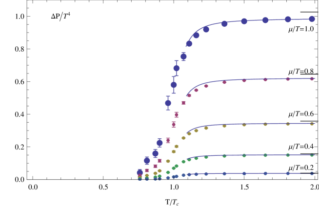
Figure 1: The reduced pressure $\Delta p/T^{4}$. The points have been obtained from lattice QCD [5].

The data points from Ref. [5] where corrected by a factor of 1.12, because as stated in Ref. [46], there should be a correction of 10-20% when extrapolating the data to the continuum. Following Letessier and Rafelski [47], the first choice for the parameter $u$ appearing in the coupling was $u=1/\pi$. However, with this value, the fit for the data below $T/T_{c}=1.2$ is quite poor. If one chooses, on the other hand, $u=1/2\pi$, agreement between lattice and the calculation presented here is satisfactory, as long as $2.7\leq\lambda_{s}\leq 3$ and $1.6\leq T_{s}\leq 2$. With these results the reduced pressure $\Delta\frac{P}{T^{4}}=\frac{P(T,\mu)-P(T,0)}{T^{4}}$ can be calculated and compared to the data. This is done in Fig. 1, with $\lambda_{s}=3$ and $T_{s}=1.98$. As seen, the agreement is quite good.

7 Conclusion

The number of different approaches that results in a consistent thermodynamics of quasi-particles, whose masses are $T$ and $\mu$ dependent, is large, as the general formalism presented here shows. The question is which one of the possible solutions is the most adequate. Or, in other words, which one allows one to get the most from it with some minimum input. Clearly, one can say that it is an advantage to work with simpler expressions, preferably with equations that allows one to make algebraic manipulations all over the calculation. And, of course, the adequate solution should be the one that reproduce both perturbative QCD and lattice QCD. Besides, it is desirable to have a solution with a field theory analogue, as for instance the $\Phi$ derivable approximation, in order to frame it in a stronger theoretical level.

From the solutions studied here, a whole class of them ($\alpha\neq 0$), which includes the Gorenstein-Yang type of solutions, have problems when a perturbative expansion is made. Specifically, although the thermodynamics consistency is achieved for the full solution, it is lost order-by-order in the perturbative expansion. This implies that this class of solutions are not able to reproduce perturbative QCD at finite $T$ and $\mu$ in any scenario. Of course, when trying to reproduce lattice data near $T_{c}$, such problem does not appear because, in that case, the full solution from the flow equation for $B$ is used, and no order-by-order approximation is made. Despite these problems, the solution GY1 has on its side the fact that the entropy density and the particle number density preserve the same form of the standard statistical mechanics, exactly as in the $\Phi$ derivable approximation. On the other hand, for the class of solutions with $\alpha=0$ (pressure is unchanged by the extra term $B$ while the other functions are modified), order-by-order thermodynamics consistency in the asymptotic limit is maintained and agreement with perturbative QCD is achieved. Moreover, the lattice QCD data is reproduced down to $T/T_{c}\sim 1.02$.

In summary, a general consistent approach for the thermodynamics of quasi-particles at finite $T$ and $\mu$ was presented for the first time. It was show that the only class of solutions for the thermodynamics functions capable to reproduce both perturbative and lattice QCD is the one where the pressure is not modified by the introduction of the extra term $B$.

This work was supported by FAPESP (04/15276-2) and CNPq (307284/2006-9).

Appendix A Appendix

The necessary integrals that appear throughout this work are:

A.1 Bose-Einstein Integrals

The Bose-Einstein integrals are [30, 48]

$$J_{n}(r)=\frac{1}{\Gamma(n)}\int_{0}^{\infty}dx\frac{x^{n-1}}{(x^{2}+r^{2})^{\frac{1}{2}}}\frac{1}{e^{(x^{2}+r^{2})^{\frac{1}{2}}}-1},\hskip 56.9055ptn>0.$$

The relevant integrals for our calculation, following [44, 45, 30] are:

$$J_{3}(r)=\frac{\pi^{2}}{12}-\frac{\pi}{4}r-\frac{r^{2}}{8}\left(\ln\frac{r}{4\pi}+\gamma_{E}-\frac{1}{2}\right)-\frac{1}{4}\sum^{\infty}_{m=1}(m+2)j_{m}r^{2(m+1)}.$$

$$J_{5}(r)=\frac{\pi^{4}}{2^{3}425}-r^{2}\frac{\pi^{2}}{96}+\frac{\pi}{48}r^{3}+\frac{r^{4}}{2^{7}}\left(\ln\frac{r}{4\pi}+\gamma_{E}-\frac{3}{4}\right)+\frac{1}{32}\sum^{\infty}_{m=1}j_{m}r^{2(m+2)}.$$

where $j_{m}=\frac{(-1)^{m}\Gamma(m+1/2)\zeta(2m+1)}{2^{2m+1}\pi^{2m}\Gamma(1/2)\Gamma(m+2)}$. The series are convergent for $r<2\pi$.

A.2 Fermi-Dirac Integrals

The Fermi-Dirac integrals are:

$$I_{n}(r,\pm{a}) = \frac{1}{\Gamma(n)}\int_{0}^{\infty}dx\frac{x^{n-1}}{\sqrt{x^{2}+r^{2}}}\frac{1}{e^{\sqrt{x^{2}+r^{2}}\pm{a}}+1},\hskip 56.9055ptn>0$$ (50)

$$G_{n}(r,\pm{a}) = \frac{1}{\Gamma(n)}\int_{0}^{\infty}dx\frac{x^{n-1}}{e^{\sqrt{x^{2}+r^{2}}\pm{a}}+1}.\hskip 108.12054ptn>0$$ (51)

As the system is composed by quarks and anti-quarks, the thermodynamics functions can be written as a linear combination of these integrals. Thus, the total integrals are:

$$I^{T}_{n}(r,a) = I_{n}(r,a)+I_{n}(r,-a),$$

$$G^{T}_{n}(r,a) = G_{n}(r,-a)-G_{n}(r,a).$$

These integrals satisfy the following recursion relations:

$$\frac{\partial{I^{T}_{n+1}(r,a)}}{\partial{r}} = -\frac{r}{n}I^{T}_{n-1}(r,a),$$ (52)

$$\frac{\partial{I^{T}_{n+1}(r,a)}}{\partial{a}} = \frac{1}{n}G^{T}_{n-1}(r,a),$$ (53)

$$\frac{\partial{G^{T}_{n+1}}(r,a)}{\partial{r}} = -\frac{r}{n}G^{T}_{n-1}(r,a),$$ (54)

$$\frac{\partial{G^{T}_{n+1}}(r,a)}{\partial{a}} = nI^{T}_{n+1}(r,a)+\frac{r^{2}}{n}{I^{T}_{n-1}(r,a)},$$ (55)

with the initial conditions

$$I^{T}_{n}(0)=\frac{2(1-2^{2-n})}{n-1}\zeta(n-1)\hskip 17.07182ptn>2,\hskip 8.5359pt\textrm{and}\hskip 17.07182ptG^{T}_{n}(0)=0\hskip 17.07182ptn>0$$ (56)

where $\zeta(n)$ is

$$\zeta(n)=\sum_{m=0}^{\infty}\frac{1}{n^{x}},\hskip 56.9055ptx>1,$$

the Riemann zeta function. The procedure to compute the integrals is inspired by Ref. [48], where bosonic integrals in the high temperature limit were computed.

If the integrals $I^{T}_{1}$ and $G^{T}_{1}$ are calculated, the recursion relations can be used to determine the remaining integrals. For the integral $I^{T}_{1}$ , the following identity is used [48]:

$$\tanh(z)=2\sum_{n=0}^{\infty}\frac{z}{z^{2}+[(n+\frac{1}{2})\pi]^{2}}=1-\frac{2}{e^{2z}+1}.$$

Thus, the Fermi-Dirac distribution is written as:

$$\frac{1}{e^{x}+1}=\frac{1}{2}-2\sum_{n=0}^{\infty}\frac{x}{x^{2}+[(2n+1)\pi]^{2}}.$$

Substituting this expression in $I^{T}_{1}$, with $x\rightarrow(x^{2}+r^{2})^{\frac{1}{2}}+a$, follows

$$I^{T}_{1}(r,a)=\int_{0}^{\infty}dx\frac{1}{\sqrt{x^{2}+r^{2}}}\left[1+\right.$$

$$\left.-2\sum_{n=1}^{\infty}\left(\frac{\sqrt{x^{2}+r^{2}}+a}{(\sqrt{x^{2}+r^{2}}+a)^{2}+[(2n+1)\pi]^{2}}+\frac{\sqrt{x^{2}+r^{2}}-a}{(\sqrt{x^{2}+r^{2}}-a)^{2}+[(2n+1)\pi]^{2}}\right)\right].$$

Manipulating the integrand to simplify the integral, one gets:

$$I^{T}_{1}(r,a)=\int_{0}^{\infty}dx\left[\frac{1}{\sqrt{x^{2}+r^{2}}}-4\sum_{n=0}^{\infty}\Re\left(\frac{1}{x^{2}+r^{2}-(a-(2n+1){\pi}i)^{2}}\right)\right]=i_{1}-4\sum_{n=0}^{\infty}i_{2,n}.$$ (57)

To solve the sub-integrals $i_{1}$ and $i_{2,n}$, it is necessary to know the solution of two specifics integrals:

$$z=\int_{0}^{\infty}dx\frac{x^{-\epsilon}}{\sqrt{x^{2}+b^{2}}}=\frac{b^{-\epsilon}}{2}B\left(\frac{1-\epsilon}{2},\frac{\epsilon}{2}\right),$$ (58)

$$w=\int_{0}^{\infty}dx\frac{x^{-\epsilon}}{x^{2}+b^{2}}=\frac{1}{2b^{1+\epsilon}}B\left(\frac{\epsilon+1}{2},\frac{1-\epsilon}{2}\right).$$ (59)

where $B(p,q)$ is the Beta function. The factor $x^{-\epsilon}$ was introduced as a convergence factor. At the end of the calculation, the limit $\epsilon\rightarrow 0$ is taken. Hence, the sub-integrals are:

$$i_{1}=\int_{0}^{\infty}dx\frac{x^{-\epsilon}}{\sqrt{x^{2}+r^{2}}}=\frac{r^{-\epsilon}}{2}B\left(\frac{1-\epsilon}{2},\frac{\epsilon}{2}\right).$$ (60)

$$i_{2,n}=\int_{0}^{\infty}dx\Re\left(\frac{x^{-\epsilon}}{x^{2}+r^{2}-(a-(2n+1){\pi}i)^{2}}\right)=\Re\left[\frac{B\left(\frac{1+\epsilon}{2},\frac{1-\epsilon}{2}\right)}{2[r^{2}-(a-(2n+1){\pi}i)^{2}]^{\frac{1+\epsilon}{2}}}\right].$$ (61)

Thus, the integral $I^{T}_{1}(r,a)$, Eq. (57), is given by:

$$I^{T}_{1}(r,a)=\frac{r^{-\epsilon}}{2}B\left(\frac{1-\epsilon}{2},\frac{\epsilon}{2}\right)-\frac{2\pi}{\sin[\frac{\pi}{2}(1-\epsilon)]}\sum^{\infty}_{n=0}\Re\left\{\frac{1}{[r^{2}-(a+(2n+1){\pi}i)^{2}]^{\frac{1+\epsilon}{2}}}\right\},$$ (62)

For $\epsilon\rightarrow 0$, the functions can be expanded in power series:

$$b^{-\epsilon}=e^{-\epsilon\ln{b}} = 1-\epsilon\ln{b}+\mathcal{O}(\epsilon^{2}),$$

$$B\left(\frac{1-\epsilon}{2},\frac{\epsilon}{2}\right) = \frac{2}{\epsilon}+\ln 4+\left(\frac{\pi^{2}}{6}+\ln^{2}2\right)\epsilon+\mathcal{O}(\epsilon^{2}),$$

$$\csc\left[\frac{\pi}{2}(1-\epsilon)\right] = 1+\mathcal{O}(\epsilon^{2}).$$ (63)

On the other hand, the denominator in the sum is rewritten as

$$\frac{1}{[r^{2}-(a+(2n+1){\pi}i)^{2}]^{\frac{1+\epsilon}{2}}}=\frac{1}{[(2n+1)\pi]^{1+\epsilon}}+\hskip 199.16928pt$$

$$+\frac{1}{[(2n+1)\pi]^{1+\epsilon}}\sum_{k=1}^{\infty}\frac{\Gamma(\frac{1+\epsilon}{2}+k)}{\Gamma(\frac{1+\epsilon}{2})\Gamma(k+1)}\left(\frac{a^{2}}{[(2n+1)\pi]^{2}}+\frac{2ai}{(2n+1)\pi}-\frac{r^{2}}{[(2n+1)\pi]^{2}}\right)^{k},$$

where a Taylor expansion was done. This expansion is valid for two cases: $a,r<\pi$ and $|\left(\frac{a^{2}}{[(2n+1)\pi]^{2}}+\frac{2ai}{(2n+1)\pi}-\frac{r^{2}}{[(2n+1)\pi]^{2}}\right)|<1$. Taking the limit $\epsilon\rightarrow 0$, one gets

$$\sum_{n=0}^{\infty}\frac{1}{[(2n+1)\pi]^{1+\epsilon}}=\frac{2^{1+\epsilon}-1}{(2\pi)^{1+\epsilon}}\zeta(1+\epsilon)=\frac{1}{2\pi}\left(\frac{1}{\epsilon}+\gamma_{E}+\ln{\frac{2}{\pi}}\right),$$

where $\gamma_{E}\approx 0.5772$ is the Euler-Mascheroni constant. The final result for $I^{T}_{1}$ is then

$$I^{T}_{1}(r,a)=-\ln\frac{r}{\pi}-\gamma_{E}-\sum_{n=0}^{\infty}\frac{2}{2n+1}\sum_{k=1}^{\infty}\frac{\Gamma(\frac{1}{2}+k)}{\Gamma(\frac{1}{2})\Gamma(k+1)}\Re\left[\left(\frac{a^{2}-r^{2}}{[(2n+1)\pi]^{2}}+\frac{2ai}{(2n+1)\pi}\right)^{k}\right].$$ (64)

The integral $I^{T}_{1}$ was also computed in [43], using the Bose integrals of Ref. [48]. In [43], however, the integral is truncated at some order. In the present calculation, there is no truncation.

To compute the $I^{T}_{3}(r,a)$ integral, one needs $G^{T}_{1}(r,a)$. Using Eq. (51)

$$G^{T}_{1}(r,a) = G_{1}(r,-a)-G_{1}(r,a)$$

$$= 2\int_{0}^{\infty}dx\sum_{n=0}^{\infty}\left[\frac{\sqrt{x^{2}+r^{2}}+a}{(\sqrt{x^{2}+r^{2}}+a)^{2}+[(2n+1)\pi]^{2}}-\frac{\sqrt{x^{2}+r^{2}}-a}{(\sqrt{x^{2}+r^{2}}-a)^{2}+[(2n+1)\pi]^{2}}\right].$$

After some manipulation,

$$G^{T}_{1}(r,a)=-4\int_{0}^{\infty}dx\sum_{n=0}^{\infty}\Re\left[\frac{a-(2n+1){\pi}i}{x^{2}+r^{2}-(a-(2n+1){\pi}i)^{2}}\right]=-4\sum_{n=0}^{\infty}{i}_{3,n}.$$ (65)

The ${i}_{3,n}$ integral is similar to $i_{2,n}$:

$${i}_{3,n}=\Re\left\{\int_{0}^{\infty}dx\frac{x^{-\epsilon}(a-(2n+1){\pi}i)}{x^{2}+r^{2}-(a-(2n+1){\pi}i)^{2}}\right\}=\frac{B\left(\frac{1+\epsilon}{2},\frac{1-\epsilon}{2}\right)}{2}\Re\left\{\frac{a-(2n+1){\pi}i}{[r^{2}-(a-(2n+1){\pi}i)^{2}]^{\frac{1+\epsilon}{2}}}\right\}.$$

As before, taking the limit $\epsilon\rightarrow 0$, one gets

$$G^{T}_{1}(r,a)=a-\frac{7a}{2}\frac{a^{2}-r^{2}}{(2\pi)^{2}}\zeta(3)+\hskip 256.0748pt$$

$$-2\sum_{n=0}^{\infty}\Re\left\{\frac{a+(2n+1){\pi}i}{2n+1}\sum_{k=2}^{\infty}\frac{\Gamma(\frac{1}{2}+k)}{\Gamma(\frac{1}{2})\Gamma(k+1)}\left(\frac{a^{2}-r^{2}}{[(2n+1)\pi]^{2}}+\frac{2ai}{(2n+1)\pi}\right)^{k}\right\}.$$ (66)

Notice that it was necessary to use both $k=0$ and $k=1$ terms in the series expansion to get a finite integral. Using the recursion relations (52) and (53), with Eqs. (64) and (66), one can easily integrate both expressions and use the initial condition Eq. (56) to obtain $I_{3}^{T}$:

$$I^{T}_{3}(r,a)=\frac{\pi^{2}}{12}+\frac{a^{2}}{4}-\frac{r^{2}}{4}\left(\frac{1}{2}-\gamma_{E}-\ln\frac{r}{\pi}\right)-\frac{7}{16}\frac{(r^{2}-a^{2})^{2}}{(2\pi)^{2}}\zeta(3)+\hskip 85.35826pt$$

$$-\sum_{n=0}^{\infty}\frac{\pi^{2}(2n+1)}{2}\sum_{k=2}^{\infty}\frac{\Gamma(\frac{1}{2}+k)}{\Gamma(\frac{1}{2})\Gamma(k+2)}\Re\left(\frac{a^{2}-r^{2}}{[(2n+1)\pi]^{2}}+\frac{2ai}{(2n+1)\pi}\right)^{k+1}.$$ (67)

To compute $G^{T}_{3}$ one needs Eqs. (54) and (55). One starts taking the derivative of the solution of Eq. (54) with respect to $a$. Then after some manipulation of this result and comparing it to Eq. (55), one gets

$$G^{T}_{3}(r,a)=\frac{\pi^{2}a}{6}+\frac{a^{3}}{6}-\frac{ar^{2}}{4}-\frac{7\zeta(3)a}{16(2\pi)^{2}}{(r^{2}-a^{2})^{2}}+\hskip 199.16928pt$$

$$-\left[\frac{21\zeta(3)a}{16(2\pi)^{2}}{(4a^{2}r^{2}-r^{4}-3a^{4})}-\frac{31\zeta(5)}{32(2\pi)^{4}}a{(r^{2}-a^{2})^{3}}\right]+\hskip 113.81102pt$$

$$-\sum_{n=0}^{\infty}[(2n+1)\pi]^{2}\Re\left\{\frac{a+(2n+1){\pi}i}{2(2n+1)}\sum_{k=3}^{\infty}\frac{\Gamma(\frac{1}{2}+k)}{\Gamma(\frac{1}{2})\Gamma(k+2)}\left(\frac{a^{2}-r^{2}}{[(2n+1)\pi]^{2}}+\frac{2ai}{(2n+1)\pi}\right)^{k+1}\right\}.$$ (68)

The second line is the contribution from $k=2$. Once $G_{3}^{T}$ is known, $I_{5}^{T}$ can be determined. From Eqs. (52) and (67), and from Eqs. (53) and (68), one has:

$$I^{T}_{5}(r,a)=\frac{7\pi^{4}}{2^{5}45}-\frac{\pi^{2}(r^{2}-2a^{2})}{96}+\frac{a^{4}}{96}-\frac{a^{2}r^{2}}{32}+\frac{r^{4}}{4^{3}}\left[\frac{3}{4}-\gamma_{E}-\ln\frac{r}{\pi}\right]+\frac{7\zeta(3)}{2^{7}3(2\pi)^{2}}(r^{2}-a^{2})^{3}+$$

$$+\left[\frac{21\zeta(3)}{2^{7}(2\pi)^{2}}a^{2}(r^{2}-a^{2})^{2}-\frac{31\zeta(5)}{2^{10}(2\pi)^{4}}(r^{2}-a^{2})^{4}\right]+\hskip 113.81102pt$$

$$-\sum_{n=0}^{\infty}\frac{\pi^{4}{(2n+1)^{3}}}{16}\sum_{k=2}^{\infty}\frac{\Gamma(\frac{1}{2}+k)}{\Gamma(\frac{1}{2})\Gamma(k+3)}\Re\left(\frac{a^{2}-r^{2}}{[(2n+1)\pi]^{2}}+\frac{2ai}{(2n+1)\pi}\right)^{k+2}.$$ (69)

.

	$\Phi$	S	N U	$\hat{N}_{T}$ $\hat{H}_{T}$	B
$\alpha=0$	$-T{\ln}Z_{T}$	$-\langle\ln\hat{\rho}\rangle-\gamma\frac{B_{S}}{T}$	$\langle\hat{N}_{T}\rangle$ $\langle\hat{H}_{T}\rangle$	$\hat{N}-\frac{\lambda}{\mu}\hat{B}_{N}$ $\sum\hat{H}-\lambda\hat{B}_{N}-\gamma\hat{B}_{S}$	$B_{S}=\frac{T}{\gamma}\sum\Big{\langle}\frac{\partial{H}}{\partial{T}}\Big{\rangle}$ $B_{N}=\frac{\mu}{\lambda}\sum\Big{\langle}\frac{\partial{H}}{\partial{\mu}}\Big{\rangle}$
$\alpha\neq 0$	$-T{\ln}Z_{T}+{\gamma}B$	$-\langle\ln\hat{\rho}\rangle-\gamma\frac{B}{T}$	$\langle\hat{N}_{T}\rangle$ $\langle\hat{H}_{T}\rangle$	$\hat{N}-\frac{\lambda}{\mu}\hat{B}$ $\sum\hat{H}-\eta\hat{B}$	$\frac{\partial}{\partial{m^{2}_{i}}}\frac{BT^{-\frac{\gamma}{\alpha}}}{\mu^{\frac{\lambda}{\alpha}}}=-\frac{T^{-\frac{\gamma}{\alpha}}}{\alpha\mu^{\frac{\lambda}{\alpha}}}\Big{\langle}\frac{\partial{H_{i}}}{\partial{m^{2}_{i}}}\Big{\rangle}$

Table 1: Summary of the two kinds of solutions for thermodynamics relations.

References

- [1] F. Wilczek, arXiv:hep-ph/0003183;
- [2] F. Karsch, Lect. Notes Phys. 583 (2002) 209,
- [3] J. C. Collins and M. J. Perry, Phys. Rev. Lett. 34 (1975) 1353.
- [4] M. Cheng et al., Phys. Rev. D 74 (2006) 054507,
- [5] C. R. Allton et al., Phys. Rev. D 71 (2005) 054508,
- [6] Z. Fodor, S. D. Katz and K. K. Szabo, Phys. Lett. B 568 (2003) 73.
- [7] M. D’Elia and M. P. Lombardo, Phys. Rev. D 70 (2004) 074509.
- [8] BRAHMS Collaboration, Nucl. Phys. A 757, 1 (2005).
- [9] PHOBOS Collaboration, Nucl. Phys. A 757, 28 (2005).
- [10] STAR Collaboration, Nucl. Phys. A 757, 102 (2005).
- [11] PHENIX Collaboration, Nucl. Phys. A 757, 184 (2005).
- [12] E. Shuryak, Prog. Part. Nucl. Phys. 53 (2004) 273.
- [13] R. Hagedorn, Nuovo Cimento 35, 395 (1965).
- [14] F. Karsch, K. Redlich and A. Tawfik, Eur. Phys. J. C 29 (2003) 549.
- [15] K. Kajantie, M. Laine, K. Rummukainen and Y. Schroder, Phys. Rev. D 67, 105008 (2003).
- [16] P. Arnold e C.-X. Zhai, Phys. Rev. D 51, 1906 (1995).
- [17] C.-X. Zhai e B. Kastening, Phys. Rev. D 52, 7232 (1995).
- [18] E. Braaten and R. D. Pisarski, Phys. Rev. D 45, 1827 (1992).
- [19] J. O. Andersen, E. Braaten and M. Strickland, Phys. Rev. Lett. 83, 2139 (1999).
- [20] J. O. Andersen, E. Braaten, E. Petitgirard and M. Strickland, Phys. Rev. D 66, 085016 (2002).
- [21] J. P. Blaizot, E. Iancu and A. Rebhan, Phys. Rev. Lett. 83, 2906 (1999).
- [22] J. P. Blaizot, E. Iancu and A. Rebhan, Phys. Rev. D 63, 065003 (2001)J. P. Blaizot, E. Iancu and A. Rebhan, arXiv:hep-ph/0303185.
- [23] A. Peshier, B. Kampfer, O. P. Pavlenko and G. Soff, Phys. Lett. B 337, 235 (1994).
- [24] P. Lévai and U. W. Heinz, Phys. Rev. C 57, 1879 (1998).
- [25] A. Peshier, B. Kampfer, O. P. Pavlenko and G. Soff, Phys. Rev. D 54, 2399 (1996).
- [26] R. A. Schneider and W. Weise, Phys. Rev. C 64, 055201 (2001).
- [27] A. Rebhan and P. Romatschke, Phys. Rev. D 68, 025022 (2003).
- [28] V. M. Bannur, Phys. Lett. B 647 (2007) 271.
- [29] V. M. Bannur, Eur. Phys. J. C 50 (2007) 629.
- [30] F. G. Gardim and F. M. Steffens, Nucl. Phys. A 797, 50 (2007).
- [31] A. Peshier and W. Cassing, Phys. Rev. Lett. 94 (2005) 172301.
- [32] M. Bluhm, B. Kampfer, R. Schulze, D. Seipt and U. Heinz, Phys. Rev. C 76, 034901 (2007).
- [33] V. M. Bannur, Phys. Rev. C 78 045206 (2008).
- [34] M. Bluhm and B. Kampfer, Phys. Rev. D 77, 114016 (2008).
- [35] S. K. Ghosh, T. K. Mukherjee, M. G. Mustafa and R. Ray, Phys. Rev. D 77, 094024 (2008).
- [36] S. Roessner, C. Ratti and W. Weise, Phys. Rev. D 75, 034007 (2007).
- [37] M. I. Gorenstein and S. N. Yang, Phys. Rev. D 52, 5206 (1995).
- [38] K. Huang, Statistical Mechanics (John Wiley e Sons, Inc., 1963).
- [39] P. Romatschke, PhD Thesis arXiv:hep-ph/0312152.
- [40] T. S. Biro, A. A. Shanenko and V. D. Toneev, Phys. Atom. Nucl. 66 (2003) 982 [Yad. Fiz. 66 (2003) 1015].
- [41] S. y. Yin and R. K. Su, arXiv:hep-th/0709.0179.
- [42] E. Fermi, Thermodynamics, Dover Publications, INC.
- [43] R. A. Schneider, arXiv:hep-ph/0303104.
- [44] J.I. Kapusta, Nucl. Phys. B 148, 461 (1979); Finite Temperature Field Theory (Cambridge University Press, Cambridge, MA, 1989).
- [45] L. Dolan and R. Jackiw, Phys. Rev. D 9, 3320 (1974).
- [46] F. Karsch, E. Laermann and A. Peikert, Phys. Lett. B 478 (2000) 447.
- [47] J. Letessier and J. Rafelski, Phys. Rev. C 67 (2003) 031902.
- [48] H. E. Haber and H. A. Weldon, J. Math. Phys. 23 (1982) 1852.
.