Theory of the Photocount Statistics for Multi-Mode Multi-Frequency Radiation Fields

Abstract

We derive on the level of quantum optics expressions for the uncertainty of the photocount in a multi-mode multi-frequency setup. The result depends on the quantum correlations of the individual modes and the frequency spectrum of the radiation, the latter leading to a frequency beating sometimes referred to as dynamic laser speckle. When the mode structure of the radiation field is disturbed between source and detector, another contribution to the photocount uncertainty referred to as static speckle appears. To predict the size of this effect, we present a suitable definition of the etendue (or phase space volume) that links the number of modes of a radiation field to macroscopic quantities.

I Introduction

Given some radiation field, a prediction can be made about the outcome of an experiment where a suitable detector is placed at some position $\vec{R}$ and probes the radiation field for some time $T$. Even when the radiation field is known as precisely as possible, there is still a finite uncertainty in the outcome. This statement can also be formulated in the inverse way: it is not possible to build an apparatus that provides a “better” (=more defined) illumination at the point $\vec{R}$ than this limit.

We will demonstrate in this paper that the uncertainty of the photocount, quantified by its variance, depends on both the number of modes, including the energy distribution among the modes, and on the spectral properties and quantum correlations of the radiation field. Another contribution to the uncertainty will appear if the radiation field is known at the source but the mode structure is then perturbed in some uncontrolled way before it reaches the location of the detector. The latter effect is frequently referred to as static speckle Goodman (2007) named after the pattern it creates on a camera. The opposing term “dynamic speckle” unfortunately is used to denote two completely different concepts in the literature. Frequently it refers to a static speckle pattern that is changing over time because the source of the perturbation is moving Fainman et al. (1981) but in this paper we refer to “dynamic laser speckle” Rydberg et al. (2006) – an effect that is due to the quantum dynamics of the radiation field.

Quantum effects are most prominent on small length scales. Modern optical lithography operates precisely in this regime, printing structures smaller than the wavelength of the light with a precision of a few nanometres Mack (2007). To this end, photo resists have been developed that are more sensitive to changes of the light intensity than most technical sensors, thereby acting as efficient (albeit unintentional) detectors for uncertainties of the photocount. Later in this paper we will show that the effects of multi-mode multi-frequency radiation are most pronounced neither at the limit of large or short times but in the intermediate regime. Recent studies have confirmed that this is precisely the regime used in modern optical lithography Noordman et al. (2009).

II Overview

Classically a radiation field is described by its electric field $\vec{E}(\vec{r},t)$ as function of position $\vec{r}$ and time $t$. In a quantum treatment, the electric field $\vec{E}$ is replaced by a suitable operator. In both treatments, the electric field is not a perfectly determined quantity, and the maximum knowledge possible is contained in the mutual-coherence function Mandel and Wolf (1995)

$$\Gamma(\vec{r}_{1},\vec{r}_{2},t_{1},t_{2})=\langle\vec{E}^{*}(\vec{r}_{1},t_{1})\vec{E}(\vec{r}_{2},t_{2})\rangle\;.$$ (1)

We restrict ourselves to stationary fields such that $\Gamma$ does not depend on $t_{1}$ and $t_{2}$ but only on the time-difference $t_{1}-t_{2}$. Furthermore, for ease of writing we will only treat one component $E$ of the electric field $\vec{E}$ but the extension to cover the other components is straight-forward.

The Fourier transform $\hat{\Gamma}(\vec{r}_{1},\vec{r}_{2},\omega)$ of $\Gamma(\vec{r}_{1},\vec{r}_{2},t_{1}-t_{2})$ with respect to the time difference is a nonnegative Hermitian operator, and thus possesses an eigenrepresentation Mandel and Wolf (1995)

$$\hat{\Gamma}(\vec{r}_{1},\vec{r}_{2},\omega)=\sum_{n}\alpha_{n}(\omega)\phi^{*}_{n}(\vec{r}_{1},\omega)\phi_{n}(\vec{r}_{2},\omega)\;,\qquad\alpha_{n}(\omega)\geq 0\;.$$ (2)

The eigenvectors $\phi_{n}(\vec{r},\omega)$ are called the modes of the electric field and form a complete orthonormal set. We assume that the frequency spectrum is small enough such that $\phi_{n}(\vec{r},\omega)$ is independent of $\omega$. Whenever the frequency spectrum is equal to the natural linewidth of the light source, i. e., the spectrum is due to the finite lifetime of some excited light-emitting medium such as in a laser, this assumption is always fulfilled. For other light sources, this assumption can sometimes be problematic for cavity-like systems but for open system or in a waveguide geometry, this is less of an issue. If the condition that $\phi_{n}(\vec{r},\omega)$ is independent of $\omega$, should be violated, one can split the mode into several discrete modes (one for each frequency interval in which the shape of the mode can assumed to be constant) and the remainder of this paper be applied nonetheless. The electric field can then be written as

$$E(\vec{r},t)=\sum_{n}a_{n}(t)\phi_{n}(\vec{r})\;.$$ (3)

Since $\phi_{n}$ is independent of $t$, the $\phi_{n}$ are the modes instead of being some arbitrary base of the electric field. Comparison of Eqs. (2) and (3) shows that the magnitude of $a_{n}$ can be computed from $\alpha_{n}$ but not its phase. A semiclassical treatment of the photocount statistics would assume that $\alpha_{n}$ is fluctuating in time whereas within quantum optics, which we will apply in this paper, fluctuations are inherent to the operator description.

This paper is organised as follows. In Sec. III we compute the variance of the photocount on a quantum-optical level when the radiation field is completely known. We will find that there is a shot noise term, a quantum correlation term and a term describing the beating of different frequencies. Frequently, by design or unintentionally, the mode structure emitted by a known light source is completely changed and unknown when it reaches the point of the detector. As will be demonstrated in Sec. V, random-matrix theory allows a compact and exact treatment of this problem. The resulting “static speckle” becomes the smaller the more modes of the radiation field are excited, and the more uniform the energy distribution among the modes is. Depending on the “size” of the radiation field, there is thus a minimum amount of static speckle, which is computed in Sec. IV. In Sec. VI we extend this question to computing the most likely amount of static speckle. Since we will demonstrate this quantity to be self-averaging, the computed average is more than just an average in that it is characteristic for almost all individual speckle values.

III Quantum theory of photodetection

While in “general” electrodynamics the electric field $\vec{E}(\vec{r},t)$ can be probed directly, this is not possible in the realm of optics as $\vec{E}(\vec{r},t)$ changes too quickly in time and space to allow a direct measurement. Rather, the radiation field is probed by means of photodetection, i. e., by absorbing photons inside some device and counting the number of photons absorbed. This principle applies to technical machines as well as to the human eye or to photo resists.

On small length and time scales, quantum effects become important. For this reason, and because all effects can then be treated in a more compact way, we will use the quantum theory of photodetection in the following. This theory Glauber (1963); Kelley and Kleiner (1964) is usually formulated for single-mode detection. Since multi-mode fields Fleischhauer and Welsch (1991) are at the core of this paper, we will present an extension of the theory to multi-mode photodetection here. We will treat the multi-frequency aspect explicitly and not express the different frequencies by different modes as is frequently done in textbooks.

We label the modes of the electromagnetic field by $\phi_{n}(\vec{r})$. The annihilation operator associated with this mode is $a_{n}$. Using this notation, the quantum operator for the electric field at some position $\vec{R}$ is given by Mandel and Wolf (1995)

$$F(t)=\sum_{n}\phi_{n}(\vec{R})a_{n}(t)\;.$$ (4)

Later it will prove helpful to switch from the time representation $a_{n}(t)$ to the spectral representation $a_{n}(\omega)$,

$$a_{n}(t)=\frac{1}{\sqrt{2\pi}}\int a_{n}(\omega)\mathrm{e}^{-\mathrm{i}\omega t}\mathrm{d}\omega\;.$$ (5)

since in time representation, operators taken at different times do not necessarily commute whereas they do in the spectral representation,

$$[a_{n}(\omega),a_{m}^{\dagger}(\omega^{\prime})]=\delta_{nm}\delta(\omega-\omega^{\prime})\;.$$ (6)

When we label the number of photons in the $n$-the mode with $I_{n}$, which basically amounts to the total intensity of that mode, this gives the expectation value

$$\langle a_{n}^{\dagger}(\omega)a_{m}(\omega)\rangle=2\pi\delta_{nm}\delta(\omega-\omega^{\prime})I_{n}G_{n}(\omega)\;,$$ (7)

where $G_{n}(\omega)$ is the (normalised) spectrum of the radiation in the $n$-th mode, and the prefactor $2\pi$ has been introduced for later convenience.

Photodetection within some time interval $T$ is then described by the quantity Mandel and Wolf (1995)

$$W=\eta\int_{0}^{T}F^{\dagger}(t)F(t)\mathrm{d}t\;,$$ (8)

where $\eta$ marks the detection efficiency and includes information on the size of the detector. This amounts to a perturbative description of the interaction between the detector and the radiation field. The perturbative approach neglects the effect that every detected photon decreases the number of photons remaining in the radiation field Fleischhauer and Welsch (1991) but this is mainly an issue for microcavities where only a small number of photons are excited at one point in time and the dynamics are then studied. For the purpose of this paper, this is no relevant restriction.

The factorial moment $n^{(k)}:=\langle n(n-1)\cdots(n-k+1)\rangle$ of the photodetection count distribution is given by

$$n^{(k)}=\langle:W^{k}:\rangle\;,$$ (9)

where the colons denote normal-ordering of the operator within, and the brackets $\langle\ldots\rangle$ denote the average which has to be taken over both the quantum fluctuations of the operators $a_{n}$ and the frequency distribution $G_{n}(\omega)$. Mean and variance of the photo count then follow from

$$\overline{n}=n^{(1)}\;,\qquad\operatorname{var}n=n^{(1)}+n^{(2)}-\bigl{[}n^{(1)}\bigr{]}^{2}\;.$$ (10)

For the first moment, this yields the result

$$n^{(1)}=\eta\langle\int_{0}^{T}\mathrm{d}t\sum_{nm}\phi_{n}^{*}(\vec{R})\phi_{m}(\vec{R})a^{\dagger}_{n}(t)a_{m}(t)\rangle=\\ \frac{\eta}{2\pi}\int_{0}^{T}\mathrm{d}t\int\!\!\!\!\int\mathrm{d}\omega_{1,2}\sum_{nm}\phi_{n}^{*}(\vec{R})\phi_{m}(\vec{R})\langle a^{\dagger}_{n}(\omega_{1})a_{m}(\omega_{2})\rangle\mathrm{e}^{\mathrm{i}(\omega_{1}-\omega_{2})t}\\ =\eta\int_{0}^{T}\mathrm{d}t\int\mathrm{d}\omega\sum_{n}\lvert\phi_{n}(\vec{R})\rvert^{2}I_{n}G_{n}(\omega)=T\eta\sum_{n}\lvert\phi_{n}(\vec{R})\rvert^{2}I_{n}\;.$$ (11)

This is the same result as expected by classical theory since $\lvert\phi_{n}(\vec{R})\rvert^{2}I_{n}$ corresponds to the intensity of the $n$-th mode at position $\vec{R}$.

The second factorial moment is

$$n^{(2)}=\eta^{2}\langle:\int\!\!\!\int_{0}^{T}\mathrm{d}t_{1,2}\sum_{n_{1},\ldots,n_{4}}\phi_{n_{1}}^{*}(\vec{R})\phi_{n_{2}}(\vec{R})\phi_{n_{3}}^{*}(\vec{R})\phi_{n_{4}}(\vec{R})a_{n_{1}}^{\dagger}(t_{1})a_{n_{2}}(t_{1})a_{n_{3}}^{\dagger}(t_{2})a_{n_{4}}(t_{2}):\rangle\\ =\frac{\eta^{2}}{4\pi^{2}}\int\!\!\!\int\!\!\!\int\!\!\!\int\mathrm{d}\omega_{1,\ldots,4}\int\!\!\!\int_{0}^{T}\mathrm{d}t_{1,2}\sum_{n_{1},\ldots,n_{4}}\phi_{n_{1}}^{*}(\vec{R})\phi_{n_{2}}(\vec{R})\phi_{n_{3}}^{*}(\vec{R})\phi_{n_{4}}(\vec{R})\langle a^{\dagger}_{n_{1}}(\omega_{1})a^{\dagger}_{n_{3}}(\omega_{3})a_{n_{2}}(\omega_{2})a_{n_{4}}(\omega_{4})\rangle\\ \times\mathrm{e}^{\mathrm{i}\bigl{[}(\omega_{1}-\omega_{2})t_{1}+(\omega_{3}-\omega_{4})t_{2}\bigr{]}}\;.$$ (12)

Taking the average over the quantum mechanical expectation operators gives nonzero contributions for three cases of the indices $n$: $n_{1}=n_{2}=n_{3}=n_{4}$, $n_{1}=n_{2}\neq n_{3}=n_{4}$, and $n_{1}=n_{4}\neq n_{2}=n_{3}$, thus

$$n^{(2)}=\frac{\eta^{2}}{4\pi^{2}}\int\!\!\!\int_{0}^{T}\mathrm{d}t_{1,2}\int\mathrm{d}\omega\sum_{n}\lvert\phi_{n}(\vec{R})\rvert^{4}\langle[a^{\dagger}_{n}(\omega)]^{2}[a_{n}(\omega)]^{2}\rangle\\ +\frac{\eta^{2}}{4\pi^{2}}\int\!\!\!\int_{0}^{T}\mathrm{d}t_{1,2}\int\mathrm{d}\omega_{1,3}\sum_{n_{1}\neq n_{3}}\lvert\phi_{n_{1}}(\vec{R})\rvert^{2}\lvert\phi_{n_{3}}(\vec{R})\rvert^{2}\langle a^{\dagger}_{n_{1}}(\omega_{1})a_{n_{1}}(\omega_{1})a^{\dagger}_{n_{3}}(\omega_{3})a_{n_{3}}(\omega_{3})\rangle\\ +\frac{\eta^{2}}{4\pi^{2}}\int\!\!\!\int\mathrm{d}\omega_{1,2}\int\!\!\!\int_{0}^{T}\mathrm{d}t_{1,2}\sum_{n_{1}\neq n_{2}}\lvert\phi_{n_{1}}(\vec{R})\rvert^{2}\lvert\phi_{n_{2}}(\vec{R})\rvert^{2}\langle a^{\dagger}_{n_{1}}(\omega_{1})a_{n_{1}}(\omega_{1})a^{\dagger}_{n_{2}}(\omega_{2})a_{n_{2}}(\omega_{2})\rangle\mathrm{e}^{\mathrm{i}\bigl{[}(\omega_{1}-\omega_{2})t_{1}+(\omega_{2}-\omega_{1})t_{2}\bigr{]}}\;.$$ (13)

This equation can be simplified by inserting the expectation values from Eq. (7). The double integral over $t_{1}$ and $t_{2}$ in the last line of Eq. (13) can be reduced to a single integral via

$$\int\!\!\!\int_{0}^{T}\mathrm{d}t_{1,2}f(t_{1}-t_{2})=\int_{-T}^{T}\mathrm{d}tf(t)[T-\lvert t\rvert]\;.$$ (14)

The remaining two integrations over $\omega_{1}$ and $\omega_{2}$ in that line each yield the Fourier transform $\hat{G}(t)$ of $G(\omega)$,

$$\hat{G}(t)=\frac{1}{\sqrt{2\pi}}\int G(\omega)\mathrm{e}^{-\mathrm{i}\omega t}\mathrm{d}t\;.$$ (15)

This thus gives

$$n^{(2)}=\frac{\eta^{2}T^{2}}{4\pi^{2}}\int\mathrm{d}\omega\sum_{n}\lvert\phi_{n}(\vec{R})\rvert^{4}\langle[a^{\dagger}_{n}(\omega)]^{2}[a_{n}(\omega)]^{2}\rangle\\ +\eta^{2}T^{2}\sum_{n_{1}\neq n_{3}}\lvert\phi_{n_{1}}(\vec{R})\rvert^{2}\lvert\phi_{n_{3}}(\vec{R})\rvert^{2}I_{n_{1}}I_{n_{3}}\\ +\frac{\eta^{2}}{2\pi}\int_{-T}^{T}\mathrm{d}t\sum_{n_{1}\neq n_{2}}\lvert\phi_{n_{1}}(\vec{R})\rvert^{2}\lvert\phi_{n_{2}}(\vec{R})\rvert^{2}\\ \times I_{n_{1}}I_{n_{2}}\hat{G}_{n_{1}}(t)\hat{G}^{*}_{n_{2}}(t)[T-\lvert t\rvert]\;.$$ (16)

The summation over $n_{1}\neq n_{3}$ is rather inconvenient. Thus, we include the missing terms $n_{1}=n_{3}$ in that summation, yielding the value $[n^{(1)}]^{2}$, and correct for this by subtracting in the first summation the terms just added. There now appears the quantity

$$f_{n}I_{n}^{2}:=\frac{1}{4\pi^{2}}\int\mathrm{d}\omega\langle[a^{\dagger}_{n}(\omega)]^{2}[a_{n}(\omega)]^{2}\rangle-\langle a^{\dagger}_{n}(\omega)a_{n}(\omega)\rangle^{2}\;,$$ (17)

that quantifies the deviation of the radiation in the $n$-th mode from a coherent state. For coherent radiation, $f_{n}=0$ since then $\langle[a^{\dagger}_{n}(\omega)]^{2}[a_{n}(\omega)]^{2}\rangle=\langle a^{\dagger}_{n}(\omega)a_{n}(\omega)\rangle^{2}$ whereas for any Gaussian light source, in particular any object emitting thermal radiation, $\langle[a^{\dagger}_{n}(\omega)]^{2}[a_{n}(\omega)]^{2}\rangle=2\langle a^{\dagger}_{n}(\omega)a_{n}(\omega)\rangle^{2}$, and $f_{n}=1$. For classical radiation, $f_{n}\geq 0$ whereas for certain nonclassical radiation $f_{n}<0$ is possible.

Collecting results, using Eq. (10), gives the variance of the photocount

$$\operatorname{var}n=\overline{n}+\eta^{2}T^{2}\sum_{n}\lvert\phi_{n}(\vec{R})\rvert^{4}I_{n}^{2}f_{n}+\\ \frac{\eta^{2}}{2\pi}\sum_{n_{1}\neq n_{2}}\lvert\phi_{n_{1}}(\vec{R})\rvert^{2}\lvert\phi_{n_{2}}(\vec{R})\rvert^{2}I_{n_{1}}I_{n_{2}}\\ \times\int_{-T}^{T}\mathrm{d}t\hat{G}_{n_{1}}(t)\hat{G}^{*}_{n_{2}}(t)[T-\lvert t\rvert]\;.$$ (18)

Equation (18) constitutes a core result of this paper. It gives the general expression for the noise that is intrinsic to any measurement of a multi-mode multi-frequency radiation field over some time $T$. The first term is the well-known shot noise term that appears naturally in the quantum treatment: electric field and photocount are quantum-optically related via the factorial moment, see Eq. (9), whereas in classical optics the relation is via the “plain” moment, with the difference between factorial and plain moments being precisely the shot-noise term.

The second term, quantified by $f_{n}$ from Eq. (17), marks the excess noise when the radiation field is not in a coherent state. As mentioned above, $f_{n}=0$ for coherent radiation, and $f_{n}=1$ for thermal radiation. Even when $f_{n}$ is small, any nonzero $f_{n}$ will eventually become the dominating effect for the photonoise as its contribution increases quadratically with time, in contrast to all other contributions. The cross-over point, where this term becomes larger than the shot-noise term, is easily estimated from Eq. (18) as $\eta Tf_{n}I_{n}\gtrsim 1$. For any thermal radiation this regime thus is already entered once the measurement time is long enough for one photon per mode to be counted on average. $I_{n}$ can be computed from the Bose-Einstein factor, evaluated at the temperature $\theta$ of the source,

$$b(\omega,\theta)=\frac{1}{\exp(\hbar\omega/k_{\mathrm{B}}\theta)-1}\;.$$ (19)

This value depends on the ratio of frequency and temperature, and thus has the same value $b\approx 0.004$ for both a light bulb emitting visible light and an EUV plasma source operating at up to $200\,000~{}\mathrm{K}$ to emit radiation with $\lambda\approx 13~{}\mathrm{nm}$.

The third and final contribution in Eq. (18) quantifies the beating of different frequency components when the measurement time is finite. It is sometimes referred to as dynamic laser speckle since it is most relevant for measurement times $T$ not much larger than the coherence time $\tau$ of the radiation,

$$\tau=\int_{-\infty}^{\infty}\mathrm{d}t\lvert\hat{G}(t)\rvert^{2}=\int_{-\infty}^{\infty}\mathrm{d}\omega\lvert G(\omega)\rvert^{2}\;,$$ (20)

hence the name “temporal degree of coherence” frequently given to $\hat{G}(t)$. However, the factor $[T-\lvert t\rvert]$ is also relevant, and it would be wrong to replace the integral simply by $\int\exp(-t/\tau)^{2}\mathrm{d}t$, as we will now demonstrate. The extra factor $[T-\lvert t\rvert]$ , which seems to be largely ignored in phenomenological literature, gives less weight to the frequently surprisingly large tails of $\hat{G}(t)$.

Two frequently encountered spectral distributions are Gaussian and Lorentzian,

$$G_{\mathrm{Gauss}}(\omega) =\sqrt{2}\tau\mathrm{e}^{-2\pi\tau^{2}\omega^{2}}\;,$$ (21)

$$G_{\mathrm{Lorentz}}(\omega) =\frac{2\tau}{1+4\pi^{2}\tau^{2}\omega^{2}}\;.$$ (22)

The curves above are already normalised to $1$, i. e., their integral (not their square integral) is $1$. The widths of the spectral distributions have been chosen such that the coherence time, computed from Eq. (20), is the same value $\tau$, allowing for a direct comparison of these two curves. Their Fourier transforms are

$$\hat{G}_{\mathrm{Gauss}}(t) =\frac{1}{\sqrt{2\pi}}\exp\Bigl{[}-\frac{t^{2}}{8\pi\tau^{2}}\Bigr{]}\;,$$ (23)

$$\hat{G}_{\mathrm{Lorentz}}(t) =\frac{1}{\sqrt{2\pi}}\exp\Bigl{[}-\frac{\lvert t\rvert}{2\pi\tau}\Bigr{]}\;.$$ (24)

The results for entering these expressions into the integral in Eq. (18) are shown in Fig. 1. There is a significant dependence on the spectral shape, with the longer tails of the Lorentzian leading to a slower approach to saturation. Please note that the graph corresponds to the variance of the photocount. When the square root of the variance is scaled by the mean intensity – this quantity is called the contrast – the saturating curve shown in the figure turns into a curve decreasing to zero as $T$ becomes larger.

$\hat{G}_{\mathrm{Lorentz}}$ is a plain exponential and thus conforms best to the simple model of how to model finite temporal coherence. We thus have used this curve for contrasting Eq. (18) by an approximation where the factor $T-\lvert t\rvert$ is replaced by $T$, thereby ignoring the additional dependence on $\lvert t\rvert$. For all values of $T$, the integral increases by about $40\,\%$, making the factor $T-\lvert t\rvert$ important for correct modelling of the photon counting statistics.

Figure 1: Value of the integral over time in Eq. (18) that quantifies the strength of the dynamic speckle. The two curves at the bottom follow by inserting the expressions for a Gaussian and a Lorentzian spectrum from Eq. (24). When the term $(T-\lvert t\rvert)$ in Eq. (18) is replaced by $T$, and an exponentially decreasing $\hat{G}(t)$ is assumed, the third curve follows.

A final word about the cross-over from “dynamics” to “statics” seems to be in order. Since the temporal effect begins to saturate at time $\tau$ it is frequently assumed that the nontemporal regime is entered once $T\gg\tau$. While this statement is correct for single-mode radiation fields, it is incorrect here since the shot-noise term $\overline{n}$, setting the reference value, scales linearly with the number $N$ of modes whereas the prefactor of the temporal term scales as $N\cdot(N-1)$ such that the condition $T\gg\tau$ has to be replaced by $T\gg N\tau$. Incidentally, since it is the regime $N\tau\gg T\gg\tau$ that current high-power excimer lasers are operating in Noordman et al. (2009), this distinction is of actual importance.

IV Etendue

Similar to classical mechanics, theoretical optics knows the concept of phase space Dragoman (2002). The optical phase space is spanned by position and spatial frequency, informally called $k$-vector, and the radiation field is completely described by the (pseudo)-density function $W(\vec{r},\vec{k})$ known as the Wigner function. Any radiation field then occupies a certain volume in phase space. Unfortunately, there is no good mathematical metric to actually measure or at least define such a volume.

In experimental and technological areas of optics, in contrast, the volume of phase space occupied is well-defined and is referred to as etendue. The energy density $I(\vec{r},\vec{\alpha})$ of the light, given as a function of position and angle, is assumed to be larger than zero only inside a finite and well-defined region. This allows for an easy and direct definition of the etendue of the radiation field. Etendue is an important quantity since, at least within geometrical optics, it can only be changed by vignetting the radiation field. The etendue supplied by some radiation field incident on some optical apparatus should thus be no larger than the etendue that this apparatus can accept.

Convolving the Wigner function $W(\vec{r},\vec{k})$ with a small kernel, its size given by an uncertainty-relation Schleich (2001), yields $I(\vec{r},\vec{\alpha})$ when the relation

$$\alpha=k\lambda\;,$$ (25)

between angle and $k$-vector is utilised. Thus on first sight it might seem that the relation between microscopic and macroscopic definition would be straight-forward.

The essential difference is that $W(\vec{r},\vec{k})$ has no finite support whereas $I(\vec{r},\vec{\alpha})$ is assumed to have. It can be shown that due to the uncertainty principle, every mode $\phi_{n}$ needs to have infinite tails in at least either real space (position) or $k$-space (angle) Folland and Sitaram (1997), and this is reflected in $W(\vec{r},\vec{k})$. Of course, also $I(\vec{r},\vec{\alpha})$ has the same infinite tails but in the macroscopic world, the function values inside those tails drop down so quickly that they are “assumed” to be zero once they are so low that they have become irrelevant for practical purposes.

We thus need a definition for phase space volume that is based on a microscopic radiation field but reduces to the macroscopic etendue for “large” radiation fields. For the purpose of this paper, the relevant way of quantifying phase space volume is by the number of modes that can be fit into it. We will tackle the problem in the opposite way: We pick a certain number of “sensible” base functions and compute all possible radiation fields that can be formed from them. We will then identify for the intensity profiles $I(\vec{r})$ as function of position and $I(\vec{\alpha})$ as a function of direction the properties that allow to deduce the number of base functions used.

To have shorter mathematical expressions, we will express directions in terms of the $k$-vector instead of the angle $\alpha$. Furthermore we make two assumptions. First, we restrict ourselves to one spatial dimension but the extension is straight-forward and becomes trivial when the radiation field factorises in its spatial dimensions. Second, we assume that the intensity distribution $I(x,k)$ factorises into a spatial term $I^{(x)}$ and an angular term $I^{(k)}$. Since the etendue accepted by practically any real-life apparatus factorises, these assumptions do not limit the applicability of this approach.

We start with $N+1$ orthonormal base functions $\phi_{n}(x)$, $n=0,\ldots,N$. The orthogonality is essential since this prevents the base functions from being too similar and thus collapsing into a very small volume of phase space. Furthermore, all modes of the radiation field have to be mutually orthogonal anyhow as they are eigenfunctions of a Hermitian operator, cf. Eq. (2). We assume them to be normalised for the ease of the calculation. For every $\phi_{n}(x)$, there also exists its Fourier transform

$$\hat{\phi}_{n}(k)=\frac{1}{\sqrt{2\pi}}\int_{-\infty}^{\infty}\phi_{n}(x)\mathrm{e}^{-\mathrm{i}kx}\mathrm{d}x\;.$$ (26)

To progress, we need to choose a certain set of base functions. The aim is to pack the base functions as tightly as possible in phase space, and without loss of generality we try to pack them around the origin. If all $\phi_{n}$, $n=0,\ldots,N$, are assumed to fulfil the conditions

$$\lvert\phi_{n}(x)\rvert \leq C(1+\lvert x\rvert)^{N}\mathrm{e}^{-a\lvert x\rvert^{2}}\;,$$ (27a)

$$\lvert\hat{\phi}_{n}(k)\rvert \leq C(1+\lvert k\rvert)^{N}\mathrm{e}^{-b\lvert k\rvert^{2}}\;,$$ (27b)

then it can be shown Hardy (1933) that $ab=1/4$ is the most condensed situation for which there are solutions. Furthermore, all solutions can then be written as

$$\phi_{n}(x)=P_{N}(x)\mathrm{e}^{-a\lvert x\rvert^{2}}\;,\qquad\hat{\phi}_{n}(k)=\tilde{P}_{N}(k)\mathrm{e}^{-b\lvert k\rvert^{2}}$$ (28)

where $P_{N}(x)$, $\tilde{P}_{N}(k)$ are polynomials of order not higher than $N$. Only the product $ab$ is fixed by this but not $a$ or $b$ on their own. This freedom is equivalent to changing $\phi_{n}(x)\to\phi_{n}(x/r)$ with the simultaneous change $\hat{\phi}_{n}(k)\to\hat{\phi}_{n}(kr)$. This also reflects that, while phase space volume is well-defined and preserved as volume, its projection onto a particular axis is allowed to change.

The set of solutions $\phi_{n}(x)$ of Eq. (28) is $N+1$ dimensional, and a convenient orthonormal set consists of the Hermite functions $\psi_{n}(x)$, defined as

$$\psi_{n}(x/r)=\frac{1}{\sqrt{n!2^{n}\sqrt{\pi}}}\exp\left[-\frac{x^{2}}{2r^{2}}\right]H_{n}(x/r)\;,$$ (29)

where $H_{n}(x)$ are the Hermite polynomials,

$$H_{0}(x)=1\;,\qquad H_{1}(x)=2x\;,\\ H_{n+1}(x)=2xH_{n}(x)-2nH_{n-1}(x)\;.$$ (30)

The prefactor in Eq. (29) ensures normalisation of $\psi_{n}(x)$. The Hermite functions are eigenfunctions of the Fourier transform,

$$\hat{\psi}_{n}(\xi r)=(-\mathrm{i})^{n}\psi_{n}(\xi/r)\;,$$ (31)

such that the derivation presented in the following for real space also applies to $k$-space.

All normalised functions $\phi(x)$ inside the solution space of Eq. (27) can be written as

$$\phi(x)=\sum_{n=0}^{N}a_{n}\psi_{n}(x)\;,\qquad\sum_{n=0}^{N}\lvert a_{n}\rvert^{2}=1\;.$$ (32)

The maximum intensity $\lvert\phi(x)\rvert^{2}$ possible for such a state can be computed using the method of Lagrange multipliers. Finding an extremum of $\phi(x)$ is equivalent to finding one of $\lvert\phi(x)\rvert^{2}$, and we will pick either of these quantities depending on which one is more convenient. The condition $\partial\Lambda/\partial a_{0}=\ldots=\partial\Lambda/\partial a_{N}=\partial\Lambda/\partial\mu=0$ of the function

$$\Lambda(a_{0},\ldots,a_{N},\mu)=\sum_{n=0}^{N}a_{n}\psi_{n}(x)-\mu(1-\sum_{n=0}^{N}\lvert a_{n}\rvert^{2})\;,$$ (33)

yields the intermediary result $\psi_{k}(x)+2\mu a_{k}=0$. By multiplying this with $\psi_{k}(x)$ respectively $a_{k}$ and summing, this gives the two conditions

$$\sum_{n=0}^{N}\lvert\psi_{n}(x)\rvert^{2} =-2\mu\sum_{n=0}^{N}a_{n}\psi_{n}(x)=-2\mu\phi(x)\;,$$ (34a)

$$-2\mu\sum_{n=0}^{N}\lvert a_{n}\rvert^{2} =\sum_{n=0}^{N}a_{n}\psi_{n}(x)=\phi(x)\;.$$ (34b)

Solving for $\mu$ by eliminating $\phi(x)$ and inserting $\mu$ into Eq. (34b), remembering that $\sum_{n=0}^{N}\lvert a_{n}\rvert^{2}=1$, one arrives at the result for the maximum intensity, namely

$$\max\lvert\phi(x)\rvert^{2}=\sum_{n=0}^{N}\lvert\psi_{n}(x)\rvert^{2}\;.$$ (35)

The method of Lagrange multipliers only gives necessary but not sufficient conditions for extrema, meaning that there cannot be any additional extrema different from Eq. (35) but this equation might not describe an extremum in the first place. Equation (35) actually describes two solutions, $\phi(x)=+\ldots$ and $\phi(x)=-\ldots$. It is obvious from physics reasons that at least two extrema, one being the most positive and one the most negative, exist. Hence, Eq. (35) uniquely describes these two extrema.

Figure 2: Maximum values $\max\lvert\phi(x)\rvert$ and $\max\lvert\hat{\phi}(k)\rvert$, computed from Eq. (35), as a function of $N$ where $N$ is the number of basis functions minus 1. Depicted are the curves for $N=1,4,9,\ldots,13^{2}$. If the corresponding curves for a normalised radiation field are below a given line, the radiation field cannot have more modes than indicated by the number $N$ on the curve.

A graphical display of the solutions $\max\lvert\phi(x)\rvert$ and $\max\lvert\hat{\phi}(x)\rvert$ can be found in Fig. 2 as a function of $N$. The right edge of $\max\lvert\phi(x)\rvert$ becomes progressively steeper as $N$ increases. This means that in the macroscopic limit $N\gg 1$ there exist a sharp edge that can be associated with the macroscopic etendue. To define the position of this edge, one could pick the $x$-coordinate where $\max\lvert\phi(x)\rvert^{2}=1/2$ or where it is equal some other particular value but this would lead to an arbitrary result. It can be shown that the number of basis functions is then proportional to the square of the width at which the “cut” is done Powell (2005) such that the result depends more on this arbitrary decision than on the radiation field. Also the method of “almost bandwidth-limited functions” (which is usually formulated for time-dependent electric signals, hence the term “bandwidth” instead of “angular range”) suffers from a similar problem Slepian (1983).

Luckily, there exists a strong link between the microscopic and macroscopic worlds because the Hermite functions $\psi_{n}(x)$ are the solutions of the eigenvalue equation

$$\frac{\mathrm{d}^{2}\psi_{n}(x)}{\mathrm{d}x^{2}}+(2n+1-x^{2})\psi_{n}(x)=0\;,$$ (36)

that can be found in any quantum mechanics textbook as it describes the harmonic oscillator. The eigenfunction $\psi_{n}$ has eigenvalue (=energy) of $n+1/2$, and a classical oscillator with the same energy is restricted to the interval $-\sqrt{2n+1}\leq x\leq\sqrt{2n+1}$. The extremal curve $\phi(x)$ computed above thus is the extremal superposition of harmonic-oscillator solutions with energy level $n$ up to $N$. Hence, the classical edge beyond which the oscillator cannot be found is given by $\sqrt{2N+1}$.

Summarising, a microscopic radiation field has at most $N+1$ modes when for all of its modes $\phi_{m}(x)$ the conditions

$$\lvert\phi_{m}(x)\rvert^{2} \leq\sum_{n=0}^{N}\lvert\psi_{n}(x/r)\rvert^{2}\;,$$ (37a)

$$\lvert\hat{\phi}_{m}(k)\rvert^{2} \leq\sum_{n=0}^{N}\lvert\psi_{n}(kr)\rvert^{2}\;,$$ (37b)

are fulfilled for some value $r$ identical for all modes. Since $\lvert\phi_{m}(x)\rvert^{2}$ and $\lvert\hat{\phi}_{m}(k)\rvert^{2}$ are the intensities as a function of position and angle, respectively, these are quantities that can in principle be measured.

A macroscopic radiation field with a half-diameter $X$ in real space and a half-diameter $K$ in angle space is thus spanned by modes $\psi_{n}$ with $n=0,\ldots,N$ determined by

$$r\sqrt{2N+1}=X\;,\qquad\frac{1}{r}\sqrt{2N+1}=K\;.$$ (38)

The scale factor $r$ drops out when expressing results in terms of the macroscopic etendue. For given etendue $E\equiv XK$, the number $N$ of modes (minus 1) is thus

$$N=\frac{E-1}{2}\;.$$ (39)

If the etendue is specified in angle (radians) instead of a $k$-vector, this becomes

$$N=\frac{E/\lambda-1}{2}\;.$$ (40)

V Static speckle

The variance of the photocount computed in Sec. III describes the uncertainty of the photocount if the radiation field at the detector is completely known. Frequently, the mode structure is known at the light source but not at the detector. The standard undergraduate example is a HeNe-laser pointed at the wall of the lecture room where the observer can see a speckle pattern. When the eyes are then moved, the direction of motion of the observed speckle pattern depends on whether the viewer is near-sighted or far-sighted Goodman (2007). The HeNe-laser emits a very regular mode structure but the modes are then changed by scattering at the rough wall. The influence of the eye movement demonstrates that scattering at the wall does not result in local intensity changes at the place of scattering but rather in a deformation of the mode structure that translates into intensity changes only by propagation to and focusing in the eye.

The change of the mode structure on its way from the radiation source to the detector can be unintentional, just as in the example above, or it can be intentional due to some apparatus designed to mix the modes of the radiation field. Unless optical systems are manufactured to the highest standards, they will have surface roughness in excess of the wavelengths. This results in uncontrolled – thus in a certain sense random – mode deformations. In addition, any apparatus designed to provide a uniform and stable illumination at its exit can only do this by means of “mixing” the incoming light. Illumination systems used in optical lithography are the supreme example of such an apparatus as the local intensity at the output varies only by about $1\,\%$ even when the form of the illumination of its entrance is completely changed. While the light paths inside such an apparatus might be very controlled, for an outside observer there (intentionally) is no recognisable connection between the light at the entrance and the exit. In other words, an apparently random change of the mode structure occurs in this case as well.

In Sec. III we have used the modes $\phi_{n}(\vec{r})$ of the radiation field to expand the operator for the electric field, cf. Eq. (4). Any orthonormal basis could have been used instead but using the modes offered the advantage that the associated annihilation operators $a_{n}(\omega)$ become uncorrelated, cf. Eq. (7). We will now switch to a different basis set, at the expense of replacing Eq. (7) by something more complicated.

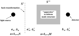
Figure 3: Graphical display of the transformation steps to arrive at static speckle. By means of a basis transformation, described by $S^{\prime}$, one switches from the modes $\phi_{n}$ that are optimal to describe the light source, to new base functions $\phi^{\prime}_{n}$ that are optimal to describe the photodetector. Along with the transformation $\phi\to\phi^{\prime}$, the annihilation operators also need to be transformed, $a\to a^{\prime}$. The additional action of scattering or mixing is then described by the matrix $S^{\prime\prime}$, transforming $a^{\prime}$ into $b$.

Considering only the radiation source and the detector, hence ignoring the scattering between them for the moment, we pick new basis functions $\phi^{\prime}_{n}(\vec{r})$ and associated annihilation operators $a^{\prime}_{n}$ such that at the location $\vec{R}$ of the detector all $\phi^{\prime}_{n}$ except for $\phi^{\prime}_{1}$ vanish. Such a basis set can always be found and offers the advantage that photodetection at the point $\vec{R}$ has been reduced to the photocount of the operator $a^{\prime}_{1}$. Since both bases are orthonormal, the transformation between $\vec{a}=a_{1},a_{2},\ldots$ and $\vec{a}^{\prime}=a^{\prime}_{1},a^{\prime}_{2},\ldots$ can be described by a unitary matrix $S^{\prime}$,

$$\vec{a}^{\prime}=S^{\prime}\vec{a}\;,$$ (41)

with $SS^{\dagger}=\openone$. Computing $S^{\prime}$ explicitly would be a very formidable task but it will turn out that knowledge of $S^{\prime}$ is not needed.

We will fix the number $M$ of new basis functions $\phi^{\prime}_{n}$ shortly but need to allow for the case that $M$ is larger than the number $N$ of excited modes of the radiation field. This is easily achieved by simply adding $M-N$ vacuum states to the input for Eq. (41).

We now assume that the radiation field is perturbed between the light source and the place of the detector by means of some “virtual device” – either intentionally by a properly designed apparatus or, usually unintentionally, by quasi-random scattering. This can be described in two opposite but physically equivalent approaches. Either, one assumes that the mode structure is perturbed, thus changing $\{\phi^{\prime}_{n}\}$ while keeping $\{a^{\prime}_{n}\}$ unchanged, or one assumes that the mode structure $\{\phi^{\prime}_{n}\}$ is unchanged while energy is transferred between modes, thus modifying $\{a^{\prime}_{n}\}$. We use the second approach, also known as the method of input-output relations Jeffers et al. (1993), since the annihilation operators $\{b_{n}\}$ describing the radiation leaving the device can then be expressed in terms of the annihilation operators $\{a^{\prime}_{n}\}$ entering device. In the absence of nonlinear media, this relation is linear, and can be described by a matrix $S^{\prime\prime}$

$$\vec{b}=S^{\prime\prime}\vec{a}^{\prime}\;.$$ (42)

If there is no absorption, $S^{\prime\prime}$ is unitary. Apart from energy conservation, already the commutation relation (6) demands the unitarity of $S$. In the presence of absorption, Eq. (42) would need to be supplemented by noise sources Jeffers et al. (1993) to ensure these commutation relations.

In the absence of further information, the unitary matrix $S^{\prime}$ describing the distortion of the mode structure is uniformly distributed in the space of unitary matrices Beenakker (1997). This concept of “maximum uncertainty” is known from other areas of physics as well, most notably from thermodynamics where the basic lemma is that every microstate compatible with the macroscopic boundary conditions is equally likely.

The photocount distribution at some point $\vec{R}$ has thus been reduced to the photocount distribution for the mode $b_{1}$, related to the original incident mode structure of the radiation source by

$$\vec{b}=S\vec{a}\;,\qquad S=S^{\prime}S^{\prime\prime}\;.$$ (43)

Since for a given position of detector and light source $\vec{R}$, $S^{\prime}$ is a fixed unitary matrix, the product $S=S^{\prime}S^{\prime\prime}$ is also distributed uniformly Mehta (1990), and so no knowledge of $S^{\prime}$ is needed, as promised above.

The only information about what happens between light source and detector enters in the form of the number $M$ of basis functions. This number is not arbitrary but is determined by the physics of the mode deformation process described by the matrix $S^{\prime\prime}$. Please remember that $M$ is the number of base functions that are mixed by the transformation $S^{\prime\prime}$. If the mode deformation is due to some intentional mixing in an apparatus accepting and emitting some etendue $E$, the number $M$ follows from the results of Sec. IV and has a finite, well-defined value. If the mode deformation is due to scattering or a diffuser, $M$ is determined by the number of basis functions that could in principle end up in the detector due to scattering or diffusing. Depending on maximum scattering angle, this can be a very large number and is always larger than $N$.

Computing the first factorial moment analogue to Eq. (11) yields

$$n^{(1)}=\eta\langle\int_{0}^{T}\mathrm{d}tb^{\dagger}_{1}(t)b_{1}(t)\rangle\\ =\eta\langle\int_{0}^{T}\mathrm{d}t\sum_{nm}a^{\dagger}_{n}(t)S^{\dagger}_{n1}S_{1m}a_{m}(t)\rangle=\eta T\sum_{n}\langle S_{1n}S^{\dagger}_{n1}\rangle I_{n}\;,$$ (44)

where in the final equality sign all averages over the fluctuations of electromagnetic field have been taken, just as described in Sec. III, and an average over the ensemble of random unitary matrices remains. The average is easily computed from $SS^{\dagger}=\openone$, hence the average in Eq. (44) is equal to $1/M$ where $M$ is the order of the matrix, yielding

$$n^{(1)}=\frac{\eta T}{M}\sum_{n}I_{n}\;.$$ (45)

This is the expected result, namely that the mean intensity at the detector is equal to the properly scaled total intensity of the original light field.

Computing the first moment demonstrated that to translate the equations from Sec. III, all terms of the form $\phi_{n}(\vec{R})$ have to be replaced by $S_{1n}$, and all terms $\phi^{*}_{n}(\vec{R})$ by $S^{\dagger}_{n1}$. The correct starting point is Eq. (16), which transforms into

$$n^{(2)}=\frac{\eta^{2}T^{2}}{4\pi^{2}}\int\mathrm{d}\omega\sum_{n}\langle\lvert S_{1n}\rvert^{4}\rangle\langle[a^{\dagger}_{n}(\omega)]^{2}[a_{n}(\omega)]^{2}\rangle\\ +\eta^{2}T^{2}\sum_{n_{1}\neq n_{3}}\langle\lvert S_{1n_{1}}\rvert^{2}\lvert S_{1n_{3}}\rvert^{2}\rangle I_{n_{1}}I_{n_{3}}\\ +\frac{\eta^{2}}{2\pi}\int_{-T}^{T}\mathrm{d}t\sum_{n_{1}\neq n_{2}}\langle\lvert S_{1n_{1}}\rvert^{2}\lvert S_{1n_{2}}\rvert^{2}\rangle\\ \times I_{n_{1}}I_{n_{2}}\hat{G}_{n_{1}}(t)\hat{G}^{*}_{n_{2}}(t)[T-\lvert t\rvert]\;.$$ (46)

It only remains to compute the necessary averages over the unitary group in a similar spirit to above where we found that $\langle S_{1n}S^{\dagger}_{n1}\rangle=1/M$. The average of the square of this expression is frequently needed and can be found in many papers, e. g. in Ref. Brouwer and Beenakker, 1996, with the result

$$\langle[S_{1n}S^{\dagger}_{n1}]^{2}\rangle=\frac{2}{M(M+1)}\;.$$ (47)

The average $\langle\lvert S_{1n}\rvert^{2}\lvert S_{1m}\rvert^{2}\rangle$ for $n\neq m$ is not identical to $\langle\lvert S_{1n}\rvert^{2}\rangle\langle\lvert S_{1m}\rvert^{2}\rangle$ as the unitary condition $SS^{\dagger}=\openone$ introduces correlations among the elements of $S$. Starting from the exact relation $1=\sum_{nm}\lvert S_{1m}\rvert^{2}\lvert S_{1n}\rvert^{2}$ allows us to write

$$\sum_{n\neq m}\langle\lvert S_{1m}\rvert^{2}\lvert S_{1n}\rvert^{2}\rangle+\sum_{n}\langle\lvert S_{1n}\rvert^{4}\rangle=1\;,$$ (48)

which, together with Eq. (47), gives us the desired average,

$$\langle\lvert S_{1n}\rvert^{2}\lvert S_{1m}\rvert^{2}\rangle=\begin{cases}\frac{1}{M(M+1)}&n\neq m\\ \frac{2}{M(M+1)}&n=m\end{cases}$$ (49)

This allows us to transform Eq. (46) into

$$n^{(2)}=\frac{\eta^{2}T^{2}}{2\pi^{2}M(M+1)}\int\mathrm{d}\omega\sum_{n}\langle[a^{\dagger}_{n}(\omega)]^{2}[a_{n}(\omega)]^{2}\rangle\\ +\frac{\eta^{2}T^{2}}{M(M+1)}\sum_{n_{1}\neq n_{3}}I_{n_{1}}I_{n_{3}}\\ +\frac{\eta^{2}}{2\pi M(M+1)}\int_{-T}^{T}\mathrm{d}t\sum_{n_{1}\neq n_{2}}I_{n_{1}}I_{n_{2}}\hat{G}_{n_{1}}(t)\hat{G}^{*}_{n_{2}}(t)[T-\lvert t\rvert]\;.$$ (50)

When computing the variance in Sec. III, the term with $I_{n_{1}}I_{n_{3}}$ dropped out when $[n^{(1)}]^{2}$ was subtracted from $n^{(2)}$. This is no longer the case here, and one arrives at

$$\operatorname{var}n=\overline{n}-\frac{1}{(M+1)}\overline{n}^{2}+\frac{\eta^{2}T^{2}}{M(M+1)}\sum_{n}(2f_{n}+1)I_{n}^{2}\\ +\frac{\eta^{2}}{2\pi M(M+1)}\int_{-T}^{T}\mathrm{d}t\sum_{n_{1}\neq n_{2}}I_{n_{1}}I_{n_{2}}\hat{G}_{n_{1}}(t)\hat{G}^{*}_{n_{2}}(t)[T-\lvert t\rvert]\;.$$ (51)

Before discussing this result, we will analyse an approximation that is frequently done: The exact averages from Eq. (49) are replaced by their Gaussian approximation, equivalent to a phasor representation Goodman (2007),

$$\langle\lvert S_{1n}\rvert^{2}\lvert S_{1m}\rvert^{2}\rangle\approx\begin{cases}\frac{1}{M^{2}}&n\neq m\\ \frac{2}{M^{2}}&n=m\end{cases}$$ (52)

The denominator in Eq. (49) was $M(M+1)$ so that the mixing of the modes would conserve energy. Equation (52) neglects this constraint. While this error might seem to be negligible for large $M$, we will demonstrate that its effect is surprisingly large. First, we compute

$$n^{(2)}\approx\frac{\eta^{2}T^{2}}{2\pi^{2}M^{2}}\int\mathrm{d}\omega\sum_{n}\langle[a^{\dagger}_{n}(\omega)]^{2}[a_{n}(\omega)]^{2}\rangle\\ +\frac{\eta^{2}T^{2}}{M^{2}}\sum_{n_{1}\neq n_{3}}I_{n_{1}}I_{n_{3}}\\ +\frac{\eta^{2}}{2\pi M^{2}}\int_{-T}^{T}\mathrm{d}t\sum_{n_{1}\neq n_{2}}I_{n_{1}}I_{n_{2}}\hat{G}_{n_{1}}(t)\hat{G}^{*}_{n_{2}}(t)[T-\lvert t\rvert]\;.$$ (53)

In contrast to Eq. (50), the term with $I_{n_{1}}I_{n_{2}}$ now cancels against $[n^{(1)}]^{2}$. The variance then becomes

$$\operatorname{var}n\approx\overline{n}+\frac{\eta^{2}T^{2}}{M^{2}}\sum_{n}(f_{n}+1)I_{n}^{2}\\ +\frac{\eta^{2}}{2\pi M^{2}}\int_{-T}^{T}\mathrm{d}t\sum_{n_{1}\neq n_{2}}I_{n_{1}}I_{n_{2}}\hat{G}_{n_{1}}(t)\hat{G}^{*}_{n_{2}}(t)[T-\lvert t\rvert]\;.$$ (54)

This is basically Eq. (18) with an additional contribution

$$\operatorname{var}n_{\mathrm{static}}\approx\frac{\eta^{2}T^{2}}{M^{2}}\sum_{n}I_{n}^{2}\;,$$ (55)

that is called “static” as its scaling with $T^{2}$ implies that its strength, when scaled by the mean squared intensity, is independent of measurement time $T$.

We arrived at the ensemble of random $S$ for calculating the variance $\operatorname{var}n_{\mathrm{static}}$ by assuming a fixed position of the detector while the mode deformations between radiation source and detector is different for a every member of the ensemble. However, from Eq. (43) it follows that this variance can equally well be computed or measured by keeping the mode formations constant while changing the position of the detector. The static speckle contrast $c$,

$$c\equiv\frac{\sqrt{\operatorname{var}n_{\mathrm{static}}}}{\overline{n}}\approx\frac{\bigl{[}\sum_{n}I_{n}^{2}]^{1/2}}{\sum_{n}I_{n}}\;,$$ (56)

can thus equally well be determined by doing a (long) measurement at different detector positions $\vec{R}$. In practise, one uses a camera instead of a point-like photodetector, and $c$ is calculated from the observed contrast of the image taken by the camera. The image resembles the speckle pattern found on the fur or skin of many animals, hence the name “speckle”. The static speckle contrast can, in this approximation, conveniently be expressed in terms of the effective number of modes $N_{\mathrm{eff}}$,

$$N_{\mathrm{eff}}=\frac{\bigl{[}\sum_{n}I_{n}]^{2}}{\sum_{n}I_{n}^{2}}\;,$$ (57)

that is equal to the actual number of modes if all intensities are equal, and smaller (implying more static speckle) otherwise.

For the exact result (51), static speckle is not so easy to define, as the difference between Eq. (51) and the results from Sec. III is not a simple term proportional to $T^{2}$. However, taking the limit $T\to\infty$, hence living up to the name “static”, the difference between these two terms gives

$$c =\frac{\bigl{[}\operatorname{var}n_{\mathrm{Eq.\,(\ref{eqTemp2exakt})}}-\operatorname{var}n_{\mathrm{Eq.\,(\ref{eqLang3})}}\bigr{]}^{1/2}}{\overline{n}}$$

$$=\left[\frac{M}{M+1}\frac{\sum_{n}I_{n}^{2}}{\bigl{[}\sum_{n}I_{n}\bigr{]}^{2}}+\frac{M-1}{M+1}\frac{\sum_{n}f_{n}I_{n}^{2}}{\bigl{[}\sum_{n}I_{n}\bigr{]}^{2}}-\frac{1}{M+1}\right]^{1/2}$$

$$=\left[\frac{M}{M+1}\Bigl{(}\frac{1}{N_{\mathrm{eff}}}-\frac{1}{M}\Bigr{)}+\frac{M-1}{M+1}\frac{\sum_{n}f_{n}I_{n}^{2}}{\bigl{[}\sum_{n}I_{n}\bigr{]}^{2}}\right]^{1/2}\;.$$ (58)

There thus is a very significant difference between the exact result and the approximation. In the latter, the contribution (55) is minimal but still nonzero if all modes carry the same intensity $I_{n}$ whereas for the exact result Eq. (51), assuming coherent radiation, this contribution vanishes if all $I_{n}$ are identical since then $N_{\mathrm{eff}}=M$.

The approximation becomes valid in the limit that there are many modes but only a small number of them are actually excited: Equation (55) depends on the average squared intensity $\langle I_{n}^{2}\rangle_{n}$ of the modes of the light source, where for a fixed light source the average is taken over its modes. This kind of average is indicated by the notation $\langle\ldots\rangle_{n}$. In contrast, the exact result Eq. (51) depends on $M/(M+1)[\langle I_{n}^{2}\rangle_{n}-\langle I_{n}\rangle_{n}^{2}]$ but the term $\langle I_{n}\rangle_{n}^{2}$ scales with the square of the fraction of excited modes and may thus be neglected in the limit stated above.

This important conclusion can also be formulated in terms of the etendue introduced in Sec. IV. The approximation is valid in the limit that the light source fills only a small fraction of the etendue that the “device” used for mixing can accept. It also means that mixing will not introduce static speckle as long as the entire etendue of the mixer is uniformly filled by the light source (assuming coherent radiation).

This might seem to contradict phenomenological theories that claim that there should aways be some pattern in the detector plane because light from the same point of the light source can reach the detector along different paths, thereby resulting in uncontrolled interference that inevitably creates intensity fluctuations. However, the unitary condition $SS^{\dagger}=\openone$ ensures that, whenever a mode of the light source is brighter at the detector, another mode has to be dimmer. This property is fulfilled for any individual $S$ since $\sum_{n}\lvert S_{1n}\rvert^{2}=1$, and no averaging over $S$ is necessary to arrive at this conclusion.

Technologically, mixing apparatuses have a well-defined etendue, hence a well-defined value of $M$. When the etendue that they can accept, is filled to a large extend by the incident radiation, the effect of the unitary condition is strong, and the exact formula (51) has to be used. For random scattering, on the other hand, in particular by a diffuser, frequently $N\ll M$, and therefore the approximate formula (55) might suffice.

VI Static speckle and etendue

In Sec. V we demonstrated that the static speckle depends on the mean squared intensity in each mode of the radiation source, hence on $\sum_{n}I_{n}^{2}$, cf. Eqs. (51) and (55). The effect is minimal if all modes carry equal weight, and the maximum number of modes possible follows from the etendue via Sec. IV. The minimum amount of static speckle possible can then be computed – it is zero if the etendue is not increased by the scattering and mixing processes, and finite otherwise.

This raises the following question: is it possible not only to compute the minimum amount of static speckle for given etendue of the radiation field but also the “typical” amount of speckle? We will demonstrate that static speckle contrast is a self-averaging quantity, i. e., in the limit of many modes $M$, the relative fluctuation while taking the average over the unitary group becomes small. This implies that the ensemble average is characteristic for almost all realisation of the ensemble.

When $\phi_{n}(\vec{r})$ are the modes of the electric field, the electric field $E(\vec{r})$ is uniquely described by coefficients $a_{n}$,

$$E(\vec{r})=\sum_{n}a_{n}\phi_{n}(\vec{r})\;,$$ (59)

and the static speckle contrast is determined by the effective number $N_{\mathrm{eff}}$ of modes in a more or less complicated way depending on whether the exact result or the approximation is used,

$$\frac{1}{N_{\mathrm{eff}}}=\frac{\sum_{n}\lvert a_{n}\rvert^{4}}{\bigl{[}\sum_{n}\lvert a_{n}\rvert^{2}\bigr{]}^{2}}\;.$$ (60)

In Sec. IV the linear span corresponding to some given etendue $E$ was computed. In the absence of dynamic information, one cannot select the modes out of all possible sets of basis vectors, and any set of basis vectors could thus represent the modes. We assume that the decomposition (59) represents the actual modes $\phi_{n}(x)$ of the radiation field. Since, as just explained, we cannot know $\phi_{n}(x)$, the equations for the static speckle contrast are instead evaluated using some other orthonormal basis $\phi^{\prime}_{n}(\vec{r})$. The two bases are related by a unitary transformation, $\vec{\phi}(\vec{r})=U\vec{\phi}^{\prime}(\vec{r})$, and consequently $\vec{a}^{\prime}=U\vec{a}$, but $U$ is unknown for the reasons just explained.

If no additional information is available, the best available estimate is the average of

$$\frac{1}{N^{\prime}_{\mathrm{eff}}} =\frac{\sum_{n}\lvert a^{\prime}_{n}\rvert^{4}}{\bigl{[}\sum_{n}\lvert a^{\prime}_{n}\rvert^{2}\bigr{]}^{2}}$$

$$=\frac{\sum_{n,i_{1},\ldots,i_{4}}U^{\dagger}_{n,i_{1}}U_{n,i_{2}}U^{\dagger}_{n,i_{3}}U_{n,i_{4}}a^{*}_{i_{1}}a_{i_{2}}a^{*}_{i_{3}}a_{i_{4}}}{\bigl{[}\sum_{n}\lvert a_{n}\rvert^{2}\bigr{]}^{2}}\;,$$ (61)

after integrating over the unitary group, i. e., over all possible unitary matrices. We study the average of $1/N^{\prime}_{\mathrm{eff}}$ instead of $N^{\prime}_{\mathrm{eff}}$ since it both is easier to compute and is the relevant quantity for the speckle contrast. The variance $\langle[1/N^{\prime}_{\mathrm{eff}}]^{2}\rangle-\langle 1/N^{\prime}_{\mathrm{eff}}\rangle^{2}$ then specifies how well the average is representative for all possible members of the ensemble.

Averaging over the unitary group, the nonvanishing terms are of the form

$$\langle U^{*}_{i_{1},j_{1}}\cdots U^{*}_{i_{M},j_{M}}U_{P(i_{1}),P^{\prime}(j_{1})}\cdots U_{P(i_{M}),P^{\prime}(j_{M})}\rangle\\ =V_{s(P^{-1}P^{\prime})}\;,$$ (62)

where $P$ and $P^{\prime}$ are permutations of the numbers $1,\ldots,M$, and $s$ denotes the cycle structure of a permutation. The coefficients $V$ depend only on the cycle structure of $P^{-1}P^{\prime}$ and have been tabulated Brouwer and Beenakker (1996).

Labelling the numerator in Eq. (61) as $Z$,

$$Z=\sum_{n}\lvert a^{\prime}_{n}\rvert^{4}=\sum_{n,i_{1},\ldots,i_{4}}U^{\dagger}_{n,i_{1}}U_{n,i_{2}}U^{\dagger}_{n,i_{3}}U_{n,i_{4}}a^{*}_{i_{1}}a_{i_{2}}a^{*}_{i_{3}}a_{i_{4}}\;,$$ (63)

and counting all the permutations of the indices in it yields

$$\langle Z\rangle=2(V_{1,1}+V_{2})\sum_{n}\sum_{i_{1},i_{3}}\lvert a_{i_{1}}\rvert^{2}\lvert a_{i_{3}}\rvert^{2}\;.$$ (64)

For the square,

$$Z^{2}=\sum_{n,m}\lvert a^{\prime}_{n}\rvert^{4}\lvert a^{\prime}_{m}\rvert^{4}\;,$$ (65)

one finds

$$\langle Z^{2}\rangle=(4V_{1,1,1,1}+24V_{2,1,1}+32V_{3,1}+12V_{2,2}+24V_{4})\times\\ \sum_{n\neq m}\sum_{i1,\ldots,i_{4}}\lvert a_{i_{1}}a_{i_{2}}a_{i_{3}}a_{i_{4}}\rvert^{2}\\ +(24V_{1,1,1,1}+144V_{2,1,1}+192V_{3,1}+72V_{2,2}+144V_{4})\times\\ \sum_{n}\sum_{i1,\ldots,i_{4}}\lvert a_{i_{1}}a_{i_{2}}a_{i_{3}}a_{i_{4}}\rvert^{2}\;.$$ (66)

The terms $a_{i_{1}},\ldots,a_{i_{4}}$ appearing in the averages above cancel against the denominator of Eq. (61). This is as expected since, as explained, these coefficients depend on the base that was used to determine them, i. e., they depend on the choice of one particular unitary matrix. Averaging over the unitary group, this choice must be irrelevant, thus the coefficients drop out, and the results depends only on the number $M$ of modes.

Inserting Eq. (64) into Eq. (61) and using the tabulated coefficients from Ref. Brouwer and Beenakker, 1996 gives the result

$$\langle\frac{1}{N^{\prime}_{\mathrm{eff}}}\rangle=\frac{2}{M+1}\;,$$ (67)

which has an easy interpretation. The term $M+1$ instead of the naive term $M$ in the denominator is due to the correlations imposed on $U$ as it is unitary, cf. the factor $M+1$ in Eq. (58). The $2$ in the numerator implies that every mode is occupied with an effective intensity of $1/2$ relative to the maximum intensity of any mode – a very plausible result since the intensity is a random quantity between $0$ and that maximum value.

A similar calculation using Eq. (66) gives for the square

$$\langle\frac{1}{{N^{\prime}_{\mathrm{eff}}}^{2}}\rangle=4\frac{M+5}{(M+1)(M+2)(M+3)}\;,$$ (68)

so that the variance becomes

$$\operatorname{var}\frac{1}{N^{\prime}_{\mathrm{eff}}}=4\frac{M-1}{(M+1)^{2}(M+2)(M+3)}\;.$$ (69)

The variance decreases much faster with $M$ than $1/N^{\prime}_{\mathrm{eff}}$ or $1/{N^{\prime}_{\mathrm{eff}}}^{2}$ as the lowest-orders in $1/M$ cancel when computing the variance. This implies that $1/N^{\prime}_{\mathrm{eff}}$ is a self-averaging quantity, and its value computed from the number $M$ and hence from the etendue of the radiation field gives a good estimation of the actual value of $1/N^{\prime}_{\mathrm{eff}}$.

One should be aware, however, that this is a statistical statement: in “almost all cases” this statement is correct. By use of particular light sources it still is possible to have a very different value for $1/N^{\prime}_{\mathrm{eff}}$. This is also reflected in the calculation presented here. Equation (60) gives the actual value of $1/N_{\mathrm{eff}}$ which, of course, depends on the values of the $a_{n}$. The average value from Eq. (67) no longer depends on the $a_{n}$ and can thus deviate.

VII Nonorthogonal modes

The modes $\phi_{n}(\vec{r})$ of the electromagnetic field are mutually orthogonal and stationary, cf. Eq. (2), and all the time-dependence of the electromagnetic field is included in the frequency-dependence of the annihilation operators. However, frequently it is rather inconvenient to describe time-dependence in this way. An extreme example are pulsed lasers where it is more appropriate to describe the mode structure of each pulse separately. This comes at a price, though, as the modes of one pulse are then not necessarily orthogonal to the modes of another pulse. This is primarily an issue for the static speckle computed in Sec. V as the mutual orthogonality of the modes was essential for the derivation presented there.

The static speckle contrast in Eq. (58) has an easy interpretation: except for a minor correction due to the unitary of the scattering matrix, every mode creates a mutually uncorrelated speckle pattern in the detector plane. The effect of a superposition of different modes is easily understood from this, and for the static part it is irrelevant if all the modes are excited simultaneously or rather one after the other. In this section, we will show that the speckle patterns of two nonorthogonal modes (i. e., necessarily at two different times) are correlated. We will, without loss of generality, refer to these two times as first and second pulse, respectively.

The first pulse consists of modes $\phi_{n}$ and annihilation operators $a_{n}$. For a fixed arrangement of mode structure of the light source, scattering between source and detector, and detector position, thus only averaging over the fluctuations of the radiation field, the mean photocount is, completely analogue to Eq. (44),

$$\overline{n}=\eta T\sum_{n}S_{1n}S^{\dagger}_{n1}I_{n}\;.$$ (70)

We now consider a second set $\phi^{\prime}_{n}$ of modes of the light source but keep the scattering between source and detector and the detector position fixed. The transformation from the $\phi_{n}$ to the $\phi^{\prime}_{n}$ is linear and can thus be described by a matrix $S^{\prime}$,

$$S^{\prime}_{kl}=\langle\phi_{k}|\phi^{\prime}_{l}\rangle\;,$$ (71)

where the notation $\langle\ldots|\ldots\rangle$ denotes the overlap integral. The annihilation operators transform as

$$a_{n}=\sum_{k}S^{\prime}_{nk}a^{\prime}_{k}\;,$$ (72)

and the mean photocount thus becomes

$$\bar{n}^{\prime}=\eta T\sum_{n}(SS^{\prime})_{1n}(SS^{\prime})^{\dagger}_{n1}I^{\prime}_{n}\;.$$ (73)

The essential quantity is the cross-correlation between $\overline{n}$ and $\bar{n}^{\prime}$ after averaging over all possible scattering configurations, hence over all $S$, and only the matrix $S^{\prime}$ may remain in the result. A positive correlation means that the light patterns caused by the two radiation fields are similar. When the photocounts of two such fields are subsequently integrated on the same detector, the static speckle contrast will be higher than naively expected by the inverse square-root of number-of-modes law.

The cross-correlation between $\overline{n}$ and $\bar{n}^{\prime}$ is given by

$$c:=\langle\overline{n}\bar{n}^{\prime}\rangle-\langle\overline{n}\rangle\langle\bar{n}^{\prime}\rangle\;,$$ (74)

and the average has to be taken over the matrix $S$ keeping the matrix $S^{\prime}$ fixed. Writing out the first term explicitly,

$$\overline{n}\bar{n}^{\prime}=\sum_{nmkl}S_{1n}S^{*}_{1n}S_{1k}S^{*}_{1l}S^{\prime}_{km}S^{\prime*}_{lm}I_{n}I^{\prime}_{m}\;,$$ (75)

the average yields nonzero terms only for $k=l$, and the two cases $k=n$ and $k\neq$ have to be distinguished. The necessary averages have already been given in Eq. (49), and the result is

$$\langle\overline{n}\bar{n}^{\prime}\rangle=\frac{2}{M(M+1)}\sum_{nm}\lvert S^{\prime}_{nm}\rvert^{2}I_{n}I^{\prime}_{m}\\ +\frac{1}{M(M+1)}\sum_{m}\sum_{n\neq k}\lvert S^{\prime}_{km}\rvert^{2}I_{n}I^{\prime}_{m}\;.$$ (76)

This can be simplified by noting that $\sum_{n\neq k}\lvert S^{\prime}_{km}\rvert^{2}=1-\lvert S^{\prime}_{nm}\rvert^{2}$. The cross-correlator then becomes

$$c=\frac{1}{M(M+1)}\sum_{nm}\left[\lvert\langle\phi_{n}|\phi^{\prime}_{m}\rangle\rvert^{2}-\frac{1}{M}\right]I_{n}I^{\prime}_{m}\;.$$ (77)

This equation gives the expected result in the two extreme situations. If all intensities are equal, the cross-correlation becomes zero since, as explained earlier in the context of Eq. (58), the static speckle itself vanishes, and thus also the cross-correlation does. If only a single mode $n$ is excited, the cross-correlation becomes proportional to $\lvert\langle\phi_{n}|\phi^{\prime}_{n}\rangle\rvert^{2}-1/M$. The average value of $\lvert\langle\phi_{n}|\phi^{\prime}_{n}\rangle\rvert^{2}$ when assuming a random $S^{\prime}$ is equal to $1/M$, and the cross-correlator is again zero. If $\phi_{n}$ and $\phi_{n}^{\prime}$ are identical, the cross-correlator becomes maximal. The cross-correlator thus correctly quantifies if $\phi_{n}$ and $\phi^{\prime}_{n}$ are stronger correlated than in a random configuration, and the overlap integral $\lvert\langle\phi_{n}|\phi^{\prime}_{m}\rangle\rvert^{2}$ is directly related to the static speckle pattern.

When a photodetector sums over $N$ pulses, the variance $\operatorname{var}n$ of the integrated photocount follows from the variances $\operatorname{var}n_{k}$ of the $k$-th pulse, given by Eq. (51), and from the cross-correlator $c_{kl}$, given by Eq. (77), between the $k$-th and the $l$-th pulse,

$$\operatorname{var}n=\sum_{k}\operatorname{var}n_{k}+\sum_{k\neq l}c_{kl}\;.$$ (78)

Apart from the rather obvious relation (78), the results from this section have another application. Frequently, radiation fields are expanded not in their modes but rather in a set of “convenient” functions, such as Gaussian beams or plane waves. Drawback of this approach is that this set then usually has to be overcomplete, hence it has more elements than there had been modes, and not all its elements are mutually orthogonal. For example, two Gaussian beams have an overlap that decreases exponentially with separation but is always larger than zero. Two plane waves restricted to a finite interval have an overlap that decreases exponentially with the angle between the two waves but is always finite.

Depending on the way that this expansion is done, some coherence information might be lost, namely when doing the expansion such that only the time-averaged intensities at all field-points are matched, and each $\phi_{n}$ is then assigned an intensity $I_{n}$. This might sound like a bad approximation but effectively amounts to using the assumptions from Sec. VI. Inserting the $I_{n}$ into Eq. (51) would yield a low static speckle contrast since the number of $I_{n}$’s is large. However, the correct equation to use is Eq. (78) where every term is evaluated for a single function $\phi_{n}$, and the nonorthogonality of the $\phi_{n}$ implies that the cross-correlation terms are large. This is as expected since introducing additional functions $\phi_{n}$ to describe the same system should not change its computed properties.

VIII Discussion

The purpose of this paper has been to give a consistent and concise description of multi-frequency and multi-mode effects on photodetection on a quantum level trying to avoid the use of uncontrolled approximations. Its focus lies on exactness, not on ease of presentation or application to some particular device. It thus complements previous work, for example by Joseph W. Goodman or the group around Christer Rydberg Rydberg et al. (2006); Goodman (2007).

In Sec. III we derived how the uncertainty of the photocount depends on the measurement time and the temporal coherence function. Among others, it was shown that a description via the coherence time of the radiation is insufficient to arrive at an exact result. Similarly, in Sec. V not only previously-known approximations of the static speckle contrast were retrieved, namely an inverse square-root law with the effective number of modes, but in addition also effects of finite etendue accepted by the “mixing device” or of noncoherent, e. g. thermal, radiation followed from the chosen mathematical formalism without additional effort.

Some of the results of this paper can be explained, albeit only on a qualitative level, by the “brick wall” model: The radiation field is like a brick wall (horizontally: time, vertically: position), and only bricks in the same column or row can cause interference effects. Counting the fraction of such bricks gives an intuitive explanation of the scaling of dynamic and static speckle contrast upon changing system parameters. If this is sufficient, the methods and results presented in this paper are a bit of an overkill. If, on the other hand, exact agreement between predication and performance of some device is essential, this paper offers the advantage of giving results using only well-defined input parameters, thus not relying on effective parameters that need to be tuned until the desired result is retrieved.

Main function of any theory is to predict whether some device or experimental setup will work as expected and / or required. For state-of-the-art technological applications, the performance might improve by about $25\,\%$ from one generation of a device or setup to the next – but rarely more. To predict if something actually is an improvement, the error due to approximations thus has to be much smaller this number. As an example, Fig. 1 gives an indication of the error made when using the coherence time instead of the exact shape of the frequency spectrum. If improvement of dynamic speckle is a topic, one should thus use the exact formulae and refrain from approximations.

Depending on the desired application, either the present paper or one of the previous works by other authors will thus be more appropriate. Furthermore, we restrict us to universal problems. For example, we study in Sec. V only the variance of the photocount, hence the contrast of the dark and bright “spots” in the plane of the detector, but not their spatial correlations, i. e., the size of these spots. Reason is that, while the contrast is universal, the size of the spots is not and depends on the setup. The book of Goodman Goodman (2007) is to a large extend devoted to studying this question (on the classical level) for a large number of setups of technological or scientific importance.

In Sec. III the uncertainty of the photocount for known radiation field has been computed, yielding in addition to the well-known shot noise term two terms depending on the frequency spectrum and on the photon correlations of the radiation source, respectively. The importance of the frequency spectrum is obvious, in particular in view of the two examples presented in this paper. For the importance of the effects of noncoherent radiation, the situation is less clear. For traditional thermal light sources, the necessary information can be found in this paper; for traditional lasers, the emitted radiation is coherent, and the question becomes trivial. For modern light sources, such as excimer lasers Basting and Marowsky (2005) that are increasingly used for high-power applications, insufficient data is available. Technological advances are fast, and no good characterisation of the photon correlations for modern devices seems to have been published. Since this contribution to the noise inevitably becomes the dominant term once the measurement time is sufficiently long, this lack of knowledge is an actual issue.

The static speckle, computed in Sec. V, depends on the number of excited modes of the radiation field (and the energy distribution among them) but, in addition, also on the number of modes that could in principle be excited. This is closely related to the concept of etendue, cf. Sec. IV. Even though etendue is a very basic quantity, its microscopic definition does not seem to have been addressed before. The relation presented between number of basis function and macroscopic etendue has application beyond this paper as any modelling of a radiation field – for the purpose of simulation or for an analytic study – needs to start with a given number of modes, and knowing this number a priori makes this process much more efficient.

While the applicability of the relation between etendue and maximum number of modes is obvious, this is less the case for Sec. VI discussing the relation between etendue and average effective number of modes. We demonstrated that this average is identical to the actual number for almost all radiation fields. However, that is “only” a statistical statement: it assumes that all possible radiation fields with given etendue are equally likely, and it is still allowed that a few cases (albeit of measure zero) deviate strongly. Different light sources have different properties, and for any technological application, one will choose the most appropriate light source. Selecting a single-mode laser that operates in a high-order Hermite-Gauss mode would give the most extreme disagreement between the actual number of modes (=one) and the prediction from Sec. VI. The results from this section can thus only be applied when the choice for a particular light source does not adversely impair the freedom of the mode structure of the generated light field.