Perfect Phylogeny Haplotyping is Complete for Logspace

Abstract

Haplotyping is the bioinformatics problem of predicting likely haplotypes based on given genotypes. It can be approached using Gusfield’s perfect phylogeny haplotyping (pph) method for which polynomial and linear time algorithms exist. These algorithm use sophisticated data structures or do a stepwise transformation of the genotype data into haplotype data and, therefore, need a linear amount of space. We are interested in the exact computational complexity of pph and show that it can be solved space-efficiently by an algorithm that needs only a logarithmic amount of space. Together with the recently proved $\operatorname{\mathchoice{\text{\small$\mathrm{L}$}}{\text{\small$\mathrm{L}$}}{\mathrm{L}}{\mathrm{L}}}$-hardness of pph, we establish $\operatorname{\mathchoice{\text{\small$\mathrm{L}$}}{\text{\small$\mathrm{L}$}}{\mathrm{L}}{\mathrm{L}}}$-completeness. Our algorithm relies on a new characterization for pph in terms of bipartite graphs, which can be used both to decide and construct perfect phylogenies for genotypes efficiently.

1 Introduction

In human genetic variation studies, sequencing methods are applied that read out the genetic information at snp (single nucleotide polymorphism) sites for multiple individuals. In order to be low-priced and feasible, these methods determine, for each site separately, the present bases, of which there can be two since the human dna is arranged in pairs of chromosomes. For each individual in the variation study this yields a genotype that describes the bases at snp sites. While the genotype says for every site which bases are present, it lacks the information on how the bases are assigned to the chromosomes of a pair. This information, which is described by haplotypes, is crucial to describe fine-grained genetic variation.

The objective of haplotyping is to compensate the drawback of genotype data by predicting biologically reasonable haplotypes computationally. Gusfield [6] proposed an approach to haplotyping that seeks haplotypes that are arrangeable in a perfect phylogenetic tree [6]. He showed that this problem, which will be called perfect phylogeny haplotyping (pph) is solvable in polynomial time by a reduction to the graph realization problem . Due to the practical importance of haplotyping, several groups also proposed simpler polynomial time [1, 4] and linear time algorithms [2, 7, 9] for Gusfield’s approach.

In the present paper we study the space complexity of pph. In [3] we showed that pph is hard for the complexity class $\operatorname{\mathchoice{\text{\small$\mathrm{L}$}}{\text{\small$\mathrm{L}$}}{\mathrm{L}}{\mathrm{L}}}$ (deterministic logarithmic space) and lies in the counting class $\operatorname{\mathchoice{\text{\small$\mathrm{\oplus L}$}}{\text{\small$\mathrm{\oplus L}$}}{\mathrm{\oplus L}}{\mathrm{\oplus L}}}$ [3] (see this paper for a wider discussion of the haplotyping issue and complexity theoretic terms). The main open problem of [3], namely, whether pph lies in the class $\operatorname{\mathchoice{\text{\small$\mathrm{L}$}}{\text{\small$\mathrm{L}$}}{\mathrm{L}}{\mathrm{L}}}$, is answered affirmatively by the present paper. To prove this result, we present a graph-based characterization that extends ideas from Eskin, Halperin and Karp [4]. Given a set of genotypes, they build, for each genotype separately, graphs where the vertices represent sites and edges represent known relations between them. Based on these graphs, they proved that the existence of a perfect phylogeny is related to the question whether one can extend the known relations, such that all graphs become complete bipartite. Our characterization avoids the step of guessing new relations between pairs of sites: We determine all relevant relations beforehand and directly construct graphs that are bipartite if, and only if, there is a perfect phylogeny. Since the graph construction can be described by first-order formulas and the problem of deciding whether a graph is bipartite lies in $\operatorname{\mathchoice{\text{\small$\mathrm{L}$}}{\text{\small$\mathrm{L}$}}{\mathrm{L}}{\mathrm{L}}}$ [8], we are able to prove the following theorem:

Theorem 1.1.

pph is complete for deterministic logarithmic space.

The paper is organized as follows: In Section 2 we provide a formal definition of the pph problem and induced sets of pairs of sites. In Section 3, we prove our graph based-characterization and, after that, we reduce pph to the problem of whether an undirected graph is bipartite in Section 4.

2 Perfect Phylogenies and Induced Sets

Since only two different bases are present at the majority of snp sites, it is convenient to code haplotypes as strings over the alphabet $\{0,1\}$, where for a given site $0$ stands for one of the bases that can be observed in practice, while $1$ encodes a second base that can also be observed. A genotype $g$ is a sequence of sets that arises from a pair of haplotypes $h$ and $h^{\prime}$ as follows: The $i$th set in the sequence $g$ is $\{h[i],h^{\prime}[i]\}$. However, it is customary to encode the set $\{0\}$ as $0$, to encode $\{1\}$ as $1$, and $\{0,1\}$ as $2$, so that a genotype is actually a string over the alphabet $\{0,1,2\}$. For example, the two haplotypes $0100$ and $0111$ underly (we also say explain) the genotype $0122$; and so do $0101$ and $0110$. These haplotype pairs differ in the way how the 2-entries at positions three and four are determined. The haplotypes have the same entries at positions three and four in the first case and different entries in the second case. This fact can be generally stated as follows: If $h$ and $h^{\prime}$ are explaining haplotypes for a genotype $g$ with 2-entries in sites $i$ and $j$ ($g[i]=g[j]=2$), then either $h[i]=h[j]\neq h^{\prime}[i]=h^{\prime}[j]$ or $h[i]=h^{\prime}[j]\neq h^{\prime}[i]=h[j]$ holds. In the first case we say that $h$ and $h^{\prime}$ resolve $g$ equally in $i$ and $j$ and in the second case we say that $h$ and $h^{\prime}$ resolve $g$ unequally in $i$ and $j$. To represent more than one haplotype, we arrange them in haplotype matrices where each row is a haplotype and each column corresponds to a site. For genotypes, we use genotype matrices. An $2n\times m$ haplotype matrix $B$ explains an $n\times m$ genotype matrix $A$ if for each $i$, the haplotypes in rows $2i-1$ and $2i$ of $B$ explain the genotype in row $i$ of $A$.

We are interested in haplotypes that are arrangeable in a perfect phylogenetic tree. We say that a haplotype matrix $B$ admits a perfect phylogeny if there exists a rooted tree $T$, such that:

1. Each row of $B$ labels exactly one node of $T$.

2. Each column of $B$ labels exactly one edge of $T$ and each edge is labeled by at least one column.

3. For every two rows $h$ and $h^{\prime}$ of $B$ and every column $i$, we have $h[i]\neq h^{\prime}[i]$ if, and only if, $i$ lies on the path from $h$ to $h^{\prime}$ in $T$.

A haplotype matrix $B$ admits a directed perfect phylogeny if $B$ together with the all-0-haplotype admits a perfect phylogeny. The four gamete property is an alternative characterization for perfect phylogenies, observed by many authors (see [5] for references). It depends on a certain relation between pairs of columns: The induced set $\operatorname{ind}^{B}(i,j)$ of two columns $i$ and $j$ in a haplotype matrix $B$ contains all strings from $\{00,01,10,11\}$ that appear in the columns $i$ and $j$. The four gamete property then says that a haplotype matrix $B$ admits a perfect phylogeny if, and only if, for each pair of columns $i$ and $j$ we have $\{00,01,10,11\}\neq\operatorname{ind}^{B}(i,j)$. Carried over to the directed case we know that $B$ admits a directed perfect phylogeny if, and only if, for each pair of columns $i$ and $j$ we have $\{01,10,11\}\nsubseteq\operatorname{ind}^{B}(i,j)$. We refer to this as the three gamete property in the following.

We say that a genotype matrix $A$ admits a (directed) perfect phylogeny if there exists an explaining haplotype matrix for it that admits a (directed) perfect phylogeny or, equivalently, satisfies the four (three) gamete property. The perfect phylogeny haplotyping problem (pph) contains exactly the genotype matrices that admit a perfect phylogeny. Similar, the directed perfect phylogeny haplotyping problem (dpph) contains exactly the genotype matrices that admit a directed perfect phylogeny. The problems pph and dpph are closely related through first-order reductions: For a reduction from dpph to pph is suffices to append the all-0-genotype to a given genotype matrix and for the converse direction we can use a reduction from Eskin, Halperin and Karp [4]: In every column where a 1-entry appears before a 0-entry, substitute all 1-entries by 0-entries and all 0-entries by 1-entries. For convenience we restrict ourselves to directed perfect phylogenies in the rest if this section and Section 3. We come back to undirected perfect phylogenies in Section 4.

A genotype matrix determines, to a certain extend, the induced sets of explaining haplotype matrices. This is formalized by the notion of induced sets for genotype matrices in [4]: For a genotype matrix $A$ and two columns $i$ and $j$, the set $\operatorname{ind}^{A}(i,j)$ contains a string $xy\in\{00,01,10,11\}$, whenever $A$ has a genotype $g$ with either $g[i]=x$ and $g[j]=y$, $g[i]=x$ and $g[j]=2$ or $g[i]=2$ and $g[j]=y$. From this definition follows that we have $\operatorname{ind}^{A}(i,j)\subseteq\operatorname{ind}^{B}(i,j)$ for any haplotype matrix $B$ explaining $A$ and $\operatorname{ind}^{A}(i,j)=\operatorname{ind}^{B}(i,j)$ if $A$ does not contain a genotype with 2-entries in both $i$ and $j$. Also we know that $A$ does not admit a directed perfect phylogeny whenever $\{01,10,11\}\subseteq\operatorname{ind}^{A}(i,j)$ holds.

If we consider only explaining haplotype matrices that satisfy the three gamete property, we can infer some information about the resolution of 2-entries: Let $A$ be a genotype matrix and $B$ an explaining haplotype matrix for $A$ that satisfies the three gamete property. Whenever we have $\{01,10\}\subseteq\operatorname{ind}^{A}(i,j)$ for columns $i$ and $j$, we know that every genotype $g$ of $A$ with $g[i]=g[j]=2$ is resolved unequally in $i$ and $j$ by its haplotypes from $B$. Whenever we have $\{11\}\subseteq\operatorname{ind}^{A}(i,j)$, the genotypes are resolved equally in $i$ and $j$. We can also infer resolutions through genotypes with at least three 2-entries: Consider a genotype $g$ from $A$ and columns $i$, $j$ and $k$ with $g[i]=g[j]=g[k]=2$ and induced sets $\{11\}\subseteq\operatorname{ind}^{A}(i,j)$ and $\{01,10\}\subseteq\operatorname{ind}^{A}(j,k)$. Let $h$ and $h^{\prime}$ be the explaining haplotypes for $g$ from $B$. We know from the induces that $h[i]=h[j]\neq h^{\prime}[i]=h^{\prime}[j]$ and $h[j]=h^{\prime}[k]\neq h^{\prime}[j]=h[k]$ hold. This implies $h[i]=h^{\prime}[k]\neq h^{\prime}[i]=h[k]$, and, therefore, every genotype with 2-entries in $i$ and $k$ must be resolved equally by its haplotypes in that columns. Note, that we do not know the resolution in columns $i$ and $k$ from the induced set of these column pair. We deduced the resolution through three 2-entries in $g$ by using information about the induced sets $\operatorname{ind}^{A}(i,j)$ and $\operatorname{ind}^{A}(j,k)$. The derived equal resolution in columns $i$ and $k$ may, again, trigger a resolution in another pair of columns $k$ and $l$ through a genotype with 2-entries in $i$, $k$ and $l$. In this way resolutions may propagate through column pairs of the whole genotype matrix. This can possibly end up with a column pair where one genotype is forced to be resolved equally, while another is already resolved unequally. In this case $A$ does not admit a perfect phylogeny. In the next section we describe graphs that represent resolutions in column pairs and their propagation through the genotype matrix.

3 A Graph-Based Characterization for Perfect Phylogeny Haplotyping

We present a new characterization for dpph in terms of undirected edge-weighted graphs. The graphs are used to represent resolutions in column pairs and their propagation in the genotype matrix. Therefore we call these graphs resolution graphs. The vertices of each resolution graph are identified with columns of a given genotype matrix and the edges are weighted by $0$ or $1$. An edge with weight $0$ between two vertices $k$ and $l$ indicates that all genotypes must be resolved equally in columns $k$ and $l$. Similar, an edge with weight $1$ indicates that the columns are resolved unequally. Our characterization in Lemma 3.1 says that the absence of odd-weight cycles (the weight of a path or a cycle is the sum of its edge weights) from the resolution graphs is equivalent to the fact that there is a directed perfect phylogeny.

Given an $n\times m$ genotype matrix $A$, we build $m$ resolution graphs, for every column $i$ a single graph $G_{i}$. A graph $G_{i}$ describes resolutions for a particular set $A_{i}$ of genotypes from $A$ and we define the $A_{i}$ sets such that they are all pairwise disjoint. If one wants to determine the haplotypes for a particular genotype $g$, it will suffice to consider the unique graph $G_{i}$ with $g\in A_{i}$. To assign the genotypes to the sets $A_{i}$, we use a partial order on genotype matrix columns from [4]: A column with index $i$ is greater than a column with index $j$ (denoted by $i\succ^{A}j$) if $\operatorname{ind}^{A}(i,j)\subseteq\{00,10,11\}$ and the column vectors are not the same (see Figure 1 for an example). Beside this partial order, we also use the total order that is given by the indices of the columns of $A$. For every $i\in\{1,\ldots,m\}$, the set $A_{i}$ is then defined as follows:

$$A_{i}=\{ \text{genotype}\ g\ \text{of}\ A\mid\ g[i]=2,$$

$$~{}~{}\forall j\neq i\ (g[j]=2\Longrightarrow\ \text{not}\ j\succ^{A}i)\ \text{and}$$

$$~{}~{}\forall j\neq i\ ((g[j]=2\ \text{and}\ \forall k\neq j\ (g[k]=2\Longrightarrow\ \text{not}\ k\succ^{A}j))\Longrightarrow\ j>i)\}\ .$$

This definition assigns every genotype with a 2-entry to exactly one set $A_{i}$. Genotypes without 2-entries do not need any resolution and, therefore, they are not assigned to any set. Figure 1 shows an example of a genotype matrix $A$ and its sets $A_{i}$.

For every $i\in\{1,\dots,m\}$, we now define the resolution graph $G_{i}$ (again, see Figure 1 for an example). As already stated, the vertices $V_{i}$ of $G_{i}$ are identified with columns from $A$. A vertex with index $k$ lies in $V_{i}$ if, and only if, $A_{i}$ contains a genotype with a 2-entry in column $k$. The edges $E_{i}\subseteq\{e\subseteq V_{i}\mid|e|=2\}$ and their weights $w_{i}:E_{i}\to\{0,1\}$ are constructed as follows:

$$\{k,l\}\in E_{i}\ \text{and}\ w_{i}(\{k,l\})=0\ \text{if, and only if, there exists}\ g_{1}\in A_{i}\ \text{with}\ g_{1}[k]=g_{1}[l]=2\ \text{and}$$

$$\text{(a)}\ 11\in\operatorname{ind}(k,l),\ \text{or}$$

$$\text{(b)}\ \text{there is a column}\ j\neq i\ \text{and}\ g_{2}\in A_{j}\ \text{with}\ g_{2}[k]=g_{2}[l]=2$$

$$\{k,l\}\in E_{i}\ \text{and}\ w_{i}(\{k,l\})=1\ \text{if, and only if, there exists}\ g_{1}\in A_{i}\ \text{with}\ g_{1}[k]=g_{1}[l]=2$$

$$\text{and}\ \{01,10\}\subseteq\operatorname{ind}^{A}(k,l)$$

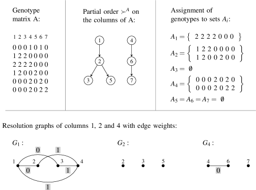
Figure 1: For a genotype matrix $A$ with seven columns, this figure shows the corresponding partial order $\succ^{A}$ on the columns of $A$, the assignment of genotypes to sets $A_{i}$, and the construction of resolution graphs $G_{i}$. Some sets $A_{i}$ are empty and, therefore, the corresponding resolution graphs are also empty. A directed edge in the partial order from a vertex with index $k$ to a vertex with index $l$ means $k\succ^{A}l$.

The characterization for dpph is as follows:

Lemma 3.1.

An $n\times m$ genotype matrix $A$ admits a directed perfect phylogeny if, and only if, for each pair $i,j\in\{1,\dots,m\}$, we have $\{01,10,11\}\nsubseteq\operatorname{ind}^{A}(i,j)$, and for each $i\in\{1,\dots,m\}$, $G_{i}$ does not contain an odd-weight cycle.

Proof.

Only-if-part: Let $A$ be a genotype matrix and $B$ a haplotype matrix for it that satisfies the three gamete property. Thus, for every pair of columns $i$ and $j$, we have $\{01,10,11\}\nsubseteq\operatorname{ind}^{B}(i,j)$ and, therefore, $\{01,10,11\}\nsubseteq\operatorname{ind}^{A}(i,j)$. To prove that none of the resolution graphs has an odd-weight cycle, we first show the following property:

Claim.

Let $A$ be a genotype matrix and $B$ a haplotype matrix for it that satisfies the three gamete property. Let $i$, $k$ and $l$ be columns and $g$ a genotype with $g\in A_{i}$ and $g[k]=g[l]=2$. If $G_{i}$ contains an edge with weight $1$ between $k$ and $l$, then $B$ resolves $g$ unequally in $k$ and $l$. If the weight is $0$, then the resolution is equal.

Proof.

If there is a $1$-weighted edge between $k$ and $l$, we have $\{01,10\}\in\operatorname{ind}^{A}(k,l)$ and, therefore, $g$ must be resolved unequally in $k$ and $l$. If there is a $0$-weighted edge between $k$ and $l$, it is constructed for one of two reason: Whenever $11\in\operatorname{ind}^{A}(k,l)$, we know by the three gamete property that $g$ must be resolved equally in $k$ and $l$. We are left with the case that there is another column $j$ and a genotype $g_{2}\in A_{j}$ with $g_{2}[k]=g_{2}[l]=2$. In this case, the following matrix shows what we know about the entries of $g_{1}$ and $g_{2}$, where $g_{1}[j]$ and $g_{2}[i]$ are values from $\{0,1,2\}$:

By definition a genotype is contained in a set $A_{i}$ if column $i$ is the maximal column (with respect to $\succ^{A}$) with the lowest index among all columns with a 2-entry in the genotype. Since $i$ and $j$ are not the same, this implies that at least one of the entries $g_{1}[j]$ and $g_{2}[i]$ does not equal 2. We distinguish between the possible values for them (possible values are $g_{2}[i]=1$, $g_{2}[i]=0$, $g_{1}[j]=1$ and $g_{1}[j]=0$) and show that we have $h_{1}[k]=h_{1}[l]\neq h_{1}^{\prime}[k]=h_{1}^{\prime}[l]$ for the explaining haplotypes $h_{1}$ and $h_{1}^{\prime}$ of $g_{1}$:

Case $g_{2}[i]=1$: We know $11\in\operatorname{ind}^{A}(i,k)$, $11\in\operatorname{ind}^{A}(i,l)$ and, therefore, $h_{1}[i]=h_{1}[k]\neq h_{1}^{\prime}[i]=h_{1}^{\prime}[k]$ and $h_{1}[i]=h_{1}[l]\neq h_{1}^{\prime}[i]=h_{1}^{\prime}[l]$ which implies $h_{1}[k]=h_{1}[l]\neq h_{1}^{\prime}[k]=h_{1}^{\prime}[l]$.

Case $g_{2}[i]=0$: By assumption column $k$ is not greater than column $i$ which implies, together with the fact that they are not the same, $10\in\operatorname{ind}^{A}(i,k)$. Similarly, we have $10\in\operatorname{ind}^{A}(i,l)$ for columns $i$ and $l$. Furthermore, the $0$-entry in $g_{2}[i]$ and the 2-entries in $g_{2}[k]$ and $g_{2}[l]$ ensure that $01\in\operatorname{ind}^{A}(i,k)$ and $01\in\operatorname{ind}^{A}(i,l)$. The resulting induced sets force an unequally resolution of $g_{1}$ in both $i$ and $k$, and $i$ and $l$. Thus $h_{1}[i]=h_{1}^{\prime}[k]\neq h_{1}^{\prime}[i]=h_{1}[k]$, $h_{1}[i]=h_{1}^{\prime}[l]\neq h_{1}^{\prime}[i]=h_{1}[l]$ and, therefore, $h_{1}[k]=h_{1}[l]\neq h_{1}^{\prime}[k]=h_{1}^{\prime}[l]$.

Case $g_{1}[j]=1$ and $g_{1}[j]=0$ are similar to case $g_{2}[i]=1$ and case $g_{2}[i]=0$, respectively. Thus, we proved the claim. ∎

We assume, for sake of contradiction, that there is a column $i$ such that $G_{i}$ contains an odd-weight cycle $i_{1},e_{1},i_{2}\dots i_{p},e_{p},i_{p+1}=i_{1}$, where the $i_{j}$ are column indices and the $e_{j}$ are weighted edges from $E_{i}$. For every edge $e_{j}$ let $g_{j}\in A_{i}$ be a genotype with $g_{j}[i_{j}]=g_{j}[i_{j+1}]=2$ and let $h_{j}$ and $h_{j}^{\prime}$ be the explaining haplotypes for $g_{j}$. The above claim and the discussion about induced sets in Section 2 imply the following two properties: First, if $h_{j}$ and $h_{j}^{\prime}$ resolve $g_{j}$ in columns $i$ and $i_{j}$ equally, then they resolve $g_{j}$ in columns $i$ and $i_{j+1}$ equally if $e_{j}$ has weight 0 and unequally, if the weight is 1. Second, if $h_{j}$ and $h_{j}^{\prime}$ resolve $g_{j}$ in columns $i$ and $i_{j}$ unequally, they resolve $g_{j}$ in columns $i$ and $i_{j+1}$ equally if $e_{j}$ has weight 1 and unequally, if the weight is 0. Thus, when an edge $e_{j}$ has weight 1, the resolution alternates between the column pair $i$ and $i_{j}$ and the column pair $i$ and $i_{j+1}$. The resolution does not alter if the weight is 0. Now assume that $g_{1}$ is resolved equally by $h_{1}$ and $h_{1}^{\prime}$ in columns $i$ and $i_{1}$. From the above property follows that for every $j\in\{1,\dots,p\}$, the genotype $g_{j}$ is resolved equally by its haplotypes in columns $i$ and $i_{j+1}$ if the path $i_{1},e_{1},i_{2}\dots i_{j},e_{j},i_{j+1}$ has an even weight, and unequally otherwise. If we consider the whole odd-weight cycle, this fact yields a contradiction to the resolution of $g_{1}$ in $i$ and $i_{1}$. The assumption that $g_{1}$ is resolved unequally in columns $i$ and $i_{1}$ is also contradictory.

If-part: Let $A$ be a genotype matrix such that for every $i$ and $j$ we have $\{01,10,11\}\nsubseteq\operatorname{ind}^{A}(i,j)$ and no resolution graph has an odd-weight cycle. We construct an explaining haplotype matrix $B$ for $A$ and show that it satisfies the three gamete property.

Construction: For genotypes without 2-entries, the explaining haplotypes are simply copies of them. The other genotypes (with 2-entries) are partitioned by the sets $A_{1},\dots,A_{m}$ and we treat every set $A_{i}$ and its graph $G_{i}$ separately. First we transform $G_{i}$ into a connected graph $G_{i}^{\prime}$: From every component that does not contain $i$, we select a vertex and connect it to $i$ by an even-weight edge. Since $G_{i}$ does not contain odd-weight cycles, each vertex is connected to $i$ by either only even-weight paths or only odd-weight paths in $G_{i}^{\prime}$. For each genotype $g\in A_{i}$, we construct two explaining haplotypes $h$ and $h^{\prime}$ as follows: For every column $j$ with $g[j]=2$, we set $h[j]=0$ and $h^{\prime}[j]=1$, if there is an even-weight path between $i$ and $j$ in $G_{i}^{\prime}$ and $h[j]=1$ and $h^{\prime}[j]=0$, otherwise. The 0-entries and 1-entries are copied to both haplotypes.

Three gamete property: We are left to prove that $\{01,10,11\}\nsubseteq\operatorname{ind}^{B}(k,l)$ holds for every column pair $k$ and $l$. If there is no genotype $g$ with 2-entries in $k$ and $l$, we simply have $\operatorname{ind}^{B}(k,l)=\operatorname{ind}^{A}(k,l)$ and the three gamete property holds for that columns by assumption. Consider two columns $k$ and $l$ that have 2-entries in a common genotype. We distinguish whether $11\in\operatorname{ind}^{A}(k,l)$, $\{01,10\}\subseteq\operatorname{ind}^{A}(k,l)$ or no of them holds and show that $\{01,10,11\}\nsubseteq\operatorname{ind}^{B}(k,l)$ is true in all cases.

1. Let $11\in\operatorname{ind}^{A}(k,l)$, $g$ a genotype with $g[k]=g[l]=2$ and $g\in A_{i}$ for a column $i$. We know that there is an edge $(0,\{k,l\})$ in $G_{i}^{\prime}$ and, therefore, either all paths from $i$ to $k$ and all paths from $i$ to $l$ have an even weight or all paths from $i$ to $k$ and all paths from $i$ to $l$ have an odd weight. The construction of the haplotypes implies that $g$ is resolved equally in $k$ and $l$. Thus, the induced set in columns $k$ and $l$ is extended only by the strings $00$ and $11$, which does not conflict with the three gamete property.

2. Let $\{01,10\}\subseteq\operatorname{ind}^{A}(k,l)$, $g$ a genotype with $g[k]=g[l]=2$ and $i$ with $g\in A_{i}$. This implies that there is an edge $(1,\{k,l\})$ in $G^{\prime}_{i}$ and, therefore, either all paths from $i$ to $k$ have an even weight and all paths from $i$ to $l$ have an odd weight or, conversely, all paths from $i$ to $k$ have an odd weight and all paths from $i$ to $l$ have an even weight. Thus, $g$ is resolved unequally by it haplotypes in $k$ and $l$, which yields the additonal induced strings $01$ and $10$.

3. Assume that neither $11\in\operatorname{ind}^{A}(k,l)$ nor $\{01,10\}\subseteq\operatorname{ind}^{A}(k,l)$ holds. If the genotypes with 2-entries in columns $k$ and $l$ lie in the same set $A_{i}$, then they are all resolved equally or all resolved unequally in $k$ and $l$, since their resolution depends on same graph $G_{i}^{\prime}$. If the genotypes with 2-entries in $k$ and $l$ are distributed among multiple sets $A_{i}$, the corresponding resolution graphs contain even-weight edges between $k$ and $l$ by definition. Similar to the first case, the construction assures that these genotypes are resolved equally in $k$ and $l$.

In all cases we proved that the resolutions of column pairs (and the resulting extension of induced sets) do not conflict with the three gamete property. ∎

4 Reduction from PPH to the Bipartition Problem

We use our characterization from the last section to show that pph can be reduced to the question of whether an undirected graph is bipartite. Bipartite graphs are characterized by the absence of an odd-length path and the formal bipartition problem contains exactly the graphs with this property.

Lemma 4.1.

pph reduces to bipartition via first-order-reductions.

Proof.

Construction: The reduction procedure consists of three steps: For a given genotype matrix $A$, we first apply the reduction from pph to dpph from [4], which is described in Section 2. This yields a genotype matrix $A^{\prime}$. Then we construct a graph $G$ that is the disjoint union of all resolution graphs of column of $A^{\prime}$. In the last step, we substitute each $0$ weighted edge in $G$ by a path of length 2 and, finally, delete all edge weights. This yields the graph $G^{\prime}$.

Correctness: First, $A$ admits a perfect phylogeny exactly if $A^{\prime}$ admits a directed perfect phylogeny. Furthermore, we know from Lemma 3.1 that $A^{\prime}$ admits a directed perfect phylogeny if, and only if, $G$ does not contain an odd-weight cycle. The insertion of paths of length 2 transforms even-weight paths into even-length paths and odd-weight paths into odd-length paths. Therefore, $G$ does not contain an odd-weight cycle if, and only if, $G^{\prime}$ is bipartite, which proves the lemma. ∎

Since ${\leavevmode\hbox{{bipartition}}}\in\operatorname{\mathchoice{\text{\small$\mathrm{L}$}}{\text{\small$\mathrm{L}$}}{\mathrm{L}}{\mathrm{L}}}$ [8] and pph is $\operatorname{\mathchoice{\text{\small$\mathrm{L}$}}{\text{\small$\mathrm{L}$}}{\mathrm{L}}{\mathrm{L}}}$-hard [3], the reduction gives the last step to prove Theorem 1.1 from the introduction.

5 Conclusion

In this paper we settled the main open problem from [3] and showed that perfect phylogeny haplotyping is solvable in deterministic logarithmic space and, therefore, is also $\operatorname{\mathchoice{\text{\small$\mathrm{L}$}}{\text{\small$\mathrm{L}$}}{\mathrm{L}}{\mathrm{L}}}$-complete (a hardness proof can be found in [3]). We introduced a characterization of pph in terms of resolution graphs that represent resolutions of 2-entries in genotypes. We proved that the question of whether there are resolutions that conflict with the existence of perfect phylogenies is closely related to the bipartition problem for undirected graphs. This yields a reduction from pph to the bipartition problem, which can be seen as a conceptual easy and efficient approach to decide and construct perfect phylogenies for genotype data.

References

- [1] V. Bafna, D. Gusfield, G. Lancia, and S. Yooseph. Haplotyping as perfect phylogeny: A direct approach. Journal of Computational Biology, 10(3–4):323–340, 2003.
- [2] Z. Ding, V. Filkov, and D. Gusfield. A linear-time algorithm for the perfect phylogeny haplotyping (PPH) problem. Journal of Computational Biology, 13(2):522–553, 2006.
- [3] M. Elberfeld and T. Tantau. Computational complexity of perfect-phylogeny-related haplotyping problems. In Proceedings of the International Symposium on Mathematical Foundations of Computer Science (MFCS 2008), volume 5162 of Lecture Notes in Computer Science, pages 299–310. Springer, 2008.
- [4] E. Eskin, E. Halperin, and R. M. Karp. Efficient reconstruction of haplotype structure via perfect phylogeny. Journal of Bioinformatics and Computational Biology, 1(1):1–20, 2003.
- [5] Jens Gramm, Arfst Nickelsen, and Till Tantau. Fixed-parameter algorithms in phylogenetics. The Computer Journal, 51(1):79–101, 2008.
- [6] D. Gusfield. Haplotyping as perfect phylogeny: Conceptual framework and efficient solutions. In Proceedings of the Sixth Annual International Conference on Computational Molecular Biology (RECOMB 2002), pages 166–175. ACM Press, 2002.
- [7] Y. Liu and C.-Q. Zhang. A linear solution for haplotype perfect phylogeny problem. In Proceedings of the International Conference on Advances in Bioinformatics and its Applications, pages 173–184. World Scientific, 2005.
- [8] O. Reingold. Undirected connectivity in log-space. Journal of the ACM, 55(4):1–24, 2008.
- [9] R. Vijaya Satya and A. Mukherjee. An optimal algorithm for perfect phylogeny haplotyping. Journal of Computational Biology, 13(4):897–928, 2006.