Scaling behavior of the contact process in networks with long-range connections

Abstract

We present simulation results for the contact process on regular, cubic networks that are composed of a one-dimensional lattice and a set of long edges with unbounded length. Networks with different sets of long edges are considered, that are characterized by different shortest-path dimensions and random-walk dimensions. We provide numerical evidence that an absorbing phase transition occurs at some finite value of the infection rate and the corresponding dynamical critical exponents depend on the underlying network. Furthermore, the time-dependent quantities exhibit log-periodic oscillations in agreement with the discrete scale invariance of the networks. In case of spreading from an initial active seed, the critical exponents are found to depend on the location of the initial seed and break the hyper-scaling law of the directed percolation universality class due to the inhomogeneity of the networks. However, if the cluster spreading quantities are averaged over initial sites the hyper-scaling law is restored.

I Introduction

It is known both for equilibrium and nonequilibrium systems that the presence of long-range interactions leads to different critical behaviors compared to universality classes characteristic for systems with short-range interactions odor . This has been demonstrated for a paradigmatic model exhibiting a phase transition to a single absorbing state, the contact process (CP), that has been introduced to model epidemic spreading without immunization ContactProcess ; GrasTor . In this simple model, lattice sites have two states (active or inactive) and active sites may become inactive or may render neighboring inactive sites active. The absorbing phase and the active phase of the systems are separated by a continuous phase transition with the universal behavior of the directed percolation (DP) DPuni ; DPuni2 ; DickMar . Long-range interactions have been included by allowing the activation process for far-away inactive sites with probabilities that decay algebraically with the distance. The critical exponents of the corresponding absorbing phase transition have been found to depend continuously on the exponent controlling the decay of activation probabilities hinrichsen ; Hbook .

An alternative way of realizing long-range interactions is when the dynamical process is defined on a network with long links that connect distant sites. Networks of this type are the scale-free networks constructed by preferential attachment Barab , where the critical behavior of CP is controlled by the degree-distribution psv ; dorog . Other models of networks are those which are composed of a $d$-dimensional regular lattice and additional long edges. These arise e.g. in sociophysics Barab or in the context of conductive properties of linear polymers with crosslinks that connect remote monomers cc . In general, a pair of nodes separated by the distance $l$ is connected by an edge with a probability $p_{l}\simeq\beta l^{-s}$ for large $l$ nw ; moukarzel ; monasson ; jespersen ; bb ; sc ; mam ; coppersmith ; kleinberg ; bh ; boettcher ; juhasz . We mention that the case $s=0$ corresponds to the Watts-Strogatz graph ws , that displays the small-world phenomenon, although that model is constructed by rewiring edges rather than adding new ones therefore the resulting graph may be disconnected. An intriguing property of these graphs for $d=1$ is that in the marginal case $s=2$, the intrinsic properties show power-law behavior and the corresponding exponents vary continuously with the prefactor $\beta$. Indeed, this has been conjectured for the diameter $D$ as a function of the number of nodes $L$, that means $D(L)\sim L^{d_{\rm min}}$ where the dimension $d_{\rm min}$ depends on $\beta$ bb . Later, power-law bounds have been established for $D(L)$ coppersmith . For a class of cubic networks with $s=2$, the algebraic growth of the diameter has been explicitly demonstrated juhasz . Moreover, the mean-square displacement of random walks in such networks has been found to grow algebraically in time with an anomalous random walk dimension that is characteristic for the underlying network. This behavior contrasts with Lévy-flights in the respect that, here, the decay exponent $s$ does not exclusively determine the diffusion exponent but the latter depends also on the details of the structure of networks if $s=2$. As opposed to random walks, much less is known for interacting many-particle systems on such networks boettcher . In particular, the behavior of nonequilibrium systems possessing an absorbing phase transition has not cleared up yet. The aim of the present work is to investigate the contact process on these networks. On the basis of the scaling of diameter and mean-square displacement of random walks, we expect a nonequilibrium system possessing an absorbing phase transition, such as the contact process, to be characterized by altered critical exponents when defined on such networks compared to the corresponding one-dimensional model. We will demonstrate by Monte Carlo simulations that this is indeed the case for a class of regular networks which, concerning the diameter and random walks, are known to be described by power-laws, similar to $s=2$ random networks. The advantage of studying regular networks is that, at least, the diameter exponent and the random-walk dimension are exactly known here and unlike for random networks no disorder (sample) average is needed to carry out here.

The rest of the paper is organized as follows. The networks to be investigated are defined in section II. The model and the studied quantities are specified in section III. Results of numerical simulations are presented in section IV and discussed in section V.

II Networks with long links

II.1 Definition of networks

In this section, we specify the networks on which the contact process is studied. First, a regular, one dimensional lattice (periodic or open) with $L$ sites is considered, where the lattice sites are numbered consecutively from $1$ to $L$. To this lattice, where the degree of sites, i.e. the number of edges emanating from a site, is $2$, links are added one by one until all sites become of degree $3$. Sites of degree $2$ will be called in brief free sites, and $k$ will denote a fixed positive integer. When constructing the networks, in general, pairs of free sites that have $k-1$ free sites between them are connected iteratively juhasz . In the following, the steps of this procedure will be described in detail.

All the networks that we study are defined by means of aperiodic sequences, therefore, we start with a brief introduction of them. The aperiodic sequences that we need are generated by substitution rules on the letters of a finite alphabet $\mathcal{A}=\{a,b,c,\dots\}$ that assigns a word (a finite string of letters) $w_{\alpha}$ to each letter $\alpha\in\mathcal{A}$. A (finite) aperiodic sequence is obtained by applying the inflation rule iteratively (finitely many times) starting with a single letter (which is letter $b$ by convention). We use the two-letter sequence defined by the inflation rule

$$\sigma_{n}:\left\{\begin{array}[]{c}{a\to w_{a}=aba(ba)^{n-1}}\\ {b\to w_{b}=a(ba)^{n-1},}\end{array}\right.$$ (1)

where $n$ is a positive integer and a three-letter sequence called tripling sequence generated by

$$\sigma_{t}:\left\{\begin{array}[]{c}{a\to w_{a}=aba}\\ {b\to w_{b}=cbc}\\ {~{}c\to w_{c}=abc.}\end{array}\right.$$ (2)

The two-letter inflation rule with $n=1$ generates the silver-mean sequence with the first few iterations $b$,$a$,$aba$,$abaaaba$,$abaaabaabaabaaaba$, etc, whereas with the choice $n=2$, the well-known Fibonacci sequence is generated.

Having defined the aperiodic sequences, we return to the construction of networks. First, the class of networks is defined where $k=1$, that means, neighboring free sites are connected recursively. Here, a finite aperiodic sequence is chosen and the edges of the (finite) initial one-dimensional lattice are labeled consecutively by the letters of this sequence. Assume that all the edges which are labeled by letter $\alpha\in\mathcal{A}$ have a common length, denoted by $l_{\alpha}$. Furthermore, let the edge lengths $l_{\alpha}$ be ordered for the case of two-letter sequences as $l_{b}<l_{a}$ while for the tripling sequence as $l_{b}<l_{c}<l_{a}$. Now, let us find the closest pair of free sites (or, to be precise, one of the pairs with the shortest spacing between them) and connect them with an additional edge. This step is then iterated until all sites become of degree $3$. It is clear that initially there is a multitude of pairs which are separated by the shortest distance ($l_{b}$) and, in the first few steps, these pairs are connected subsequently. Obviously, as the procedure goes on, the minimal spacing increases and longer and longer edges will form.

We have studied the contact process on three different networks with $k=1$: the silver-mean network, the Fibonacci network and the tripling network, which are constructed by using the corresponding aperiodic sequence. The structure of these networks is illustrated in Fig. 1.

Figure 1: Finite silver-mean, Fibonacci and tripling networks (from top to bottom).

In addition to this, we have considered networks with $k=2$, as well. The $k=2$ tripling network and the $k=2$ silver-mean network are constructed as follows juhasz . First, the sites of a one-dimensional lattice are labeled with the letters of the corresponding sequence. The sites are grouped into blocks corresponding to words $w_{\alpha}$ in the inflation rule. Then, sites belonging to one-letter blocks are renamed according to the reversed inflation rule $w_{\alpha}\to\alpha$, where $w_{\alpha}$ is the one-letter word corresponding to the block. In blocks composed of three sites, the two lateral sites are connected, and the middle one is renamed again according to the reversed inflation rule $w_{\alpha}\to\alpha$, where $w_{\alpha}$ is the word corresponding to the block. The above step is then iterated until only one free site (the central one) is left.

Figure 2: Finite $k=2$ tripling, silver-mean and Hanoi-tower networks (from top to bottom).

The third network with $k=2$ that will be investigated is the cubic Hanoi-tower network boettcher that can be constructed following the above procedure with the inflation rule

$$\sigma_{H}:\left\{\begin{array}[]{c}{a\to w_{a}=aba}\\ {b\to w_{b}=b.}\end{array}\right.$$ (3)

The three networks with $k=2$ are illustrated in Fig. 2.

II.2 Diameter and random-walk dimension

In the rest of this section, we shall survey some intrinsic properties of the above networks that are exactly known and are relevant with respect to the off-critical dynamical behavior of the contact process.

Beside the distance $x$ measured on the underlying one-dimensional lattice, another metric is the shortest-path length $\ell$ between two sites which is the minimal number of links that have to be traversed when going from one site to the other one. The average length of the shortest path between two sites separated by the distance $x$ scales in these networks as $\overline{\ell}(t)\sim x^{d_{\rm min}}$ where $d_{\rm min}$ is the shortest-path dimension of the network. The diameter $D(L)$ of a typical finite graph with $L$ sites, which is the largest shortest-path length between any two sites grows also algebraically as $D(L)\sim L^{d_{\rm min}}$. The average number of sites $V(\ell)$ that can be reached in at most $\ell$ steps starting from a given site scales as $V(\ell)\sim\ell^{d_{g}}$ where $d_{g}$ is the graph dimension that is related to $d_{\rm min}$ as $d_{g}=1/d_{\rm min}$.

The other property that we need is the random-walk dimension of the network. Let us consider a continuous time random walk on (infinite) networks, where the walker can jump with unit rate to any of the sites connected with the site it resides. The random-walk dimension $d_{w}$ is defined through the asymptotical relation $[\langle x^{2}(t)\rangle]_{\rm typ}\sim t^{2/d_{w}}$, where $x(t)$ denotes the displacement of the walker at time $t$ and $[\langle x^{2}(t)\rangle]_{\rm typ}\equiv\exp{\overline{\ln\langle x^{2}(t)\rangle}}$ is the “typical value” of $\langle x^{2}(t)\rangle$. Here, $\langle\cdot\rangle$ denotes the average over different stochastic histories for a fixed starting position, while the over-bar stands for the average over starting positions. Note that the expected value $\overline{\langle x^{2}(t)\rangle}$ does not exist if $t>0$ since the expected value of edge lengths is infinite (in infinite networks). This accounts for that the average of $\ln\langle x^{2}(t)\rangle$ is considered instead. Notice that $d_{\rm rw}$ is a dynamical exponent that relates time and length scale of random walks.

The dimensions $d_{\rm min}$ and $d_{\rm rw}$ of the networks defined in the previous section have been exactly calculated boettcher ; juhasz ; the corresponding numerical values are shown in Table 1 and Table 2.

III Contact process on networks

III.1 Definition of the model

The contact process is one of the earliest and simplest lattice models that belongs to the DP universality class. It is a continuous time Markov process on a state space $\{0,1\}^{S}$, where $S$ is a finite or countable graph, usually $\mathbb{Z}^{d}$. A site with state $0$($1$) is called inactive(active) or, in the context of epidemics, healthy(infected). The dynamics is defined by nearest-neighbor transitions that occur independently with given rates. In $d$ dimension, an infected site can spontaneously become healthy ($1\to 0$) with rate $1$ or can infect one of its neighbors ($0\to 1$) with rate $\lambda/(2d)$ (see Fig. 3). This process is defined on the cubic networks under consideration in the way that infected sites are healed with rate $1$ as before, whereas each nearest-neighbor site is infected with rate $\lambda/3$, such that (for a site of degree $3$) the total infection rate is $\lambda$.

Figure 3: Allowed transitions and the corresponding rates in the one-dimensional contact process. Full(empty) circles symbolize active(inactive) sites.

In numerical simulations, this process is realized by random sequential updates: a randomly chosen infected site either becomes healthy with probability $1/(1+\lambda)$ or a neighboring site is attempted to be infected with probability $\lambda/[3(1+\lambda)]$. For sites of degree $2$ (the central site in $k=2$ networks and the surface sites in open $k=2$ networks) and for sites of degree $1$ (the surface sites in $k=1$ networks), no update is attempted with probability $\lambda/[3(1+\lambda)]$ and $2\lambda/[3(1+\lambda)]$, respectively.

Throughout the paper we measure the time in units of Monte Carlo (MC) steps that corresponds to $N$ update attempts, where $N$ is the actual number of particles at the beginning of the MC step.

III.2 Studied quantities

The quantities, the time-dependence of which we have measured at criticality, are the average number of active sites $N(t)$ and the survival probability $P(t)$, which is the probability that there is at least one active site at time $t$. Furthermore, in the case of seed simulations, when initially a single site denoted by $m$ is active and all other sites are inactive, we have also measured the second moment of the distance of the growing cluster with respect to the origin $m$, the so called spread $R_{m}^{2}(t)$. To be precise, this quantity is defined as $R_{m}^{2}(t)=\langle\sum_{i=1}^{L}n_{i}(t)x_{i}^{2}(t)\rangle/N(t)$, where $x_{i}$ is the distance between site $i$ and the origin $m$, whereas $n_{i}$ is a binary variable which is one(zero) for active(inactive) sites. In the case of a single initial seed, the above quantities are expected to follow power-laws asymptotically:

$$N_{m}(t)\sim t^{\eta_{m}}$$ (4)

$$P_{m}(t)\sim t^{-\delta_{m}}$$ (5)

$$R_{m}^{2}(t)\sim t^{2/z_{m}}.$$ (6)

In an inhomogeneous system the critical exponents $\eta_{m}$, $\delta_{m}$ and $z_{m}$ may be different for different initial active sites $m$. We shall see, that this is indeed the case, at least for the former two exponents. We have probed three different positions for the initial seed. First, it has been located at the central site(s), i.e. site $(L+1)/2$ for $k=2$ networks, where the number of sites $L$ is odd, and sites $L/2$ and $L/2+1$ for $k=1$, where $L$ is even. We shall refer to this arrangement of the initial seed by the index ’$0$’. Second, the initial seed has also been located at the site from which the longest edge of the (finite) network emanates. (Note that the edge connecting site $1$ and site $L$ in Fig. 1 is not the longest one since they are neighbors on the ring.) This initialization is indexed by ’$l$’. Note that in this case, as the process starts, the spread jumps immediately to $O(x^{2})$, where $x$ is the length of the longest edge. To ensure the smooth increase of the spread, we have modified its definition so that $x_{i}$ is the minimum of the distances measured from the two sites which are connected by the longest edge. Third, we have considered networks built on open one-dimensional chains, where the end sites are of degree $1$ for $k=1$ and of degree $2$ for $k=2$. In these networks, the initial seed has been located at the surface, i.e. at site $1$. The exponents corresponding to this arrangement are indexed by ’s’.

In addition to this, we have measured $\overline{N(t)}$ and $\overline{P(t)}$, the number of active sites and the survival probability, respectively, that are averaged over seed simulations started from all possible initial sites $1,2,\dots,L$. The corresponding exponents are denoted by $\eta_{\rm av}$ and $\delta_{\rm av}$. Note that the average of $R^{2}(t)$ over all possible initial sites diverges in an infinite network for any $t>0$ since the expected value of edge-lengths is infinite juhasz . Nevertheless, the averaging would not provide any new information anyway on the spread since, according to the numerical results, the dynamical exponent $z_{m}\equiv z$ is independent of the location of the initial seed.

Another dynamical scaling exponent characterizes the critical system that is started from a homogeneous, fully occupied initial state. In this case, the density $\rho(t)$ of infected sites decays asymptotically as

$$\rho(t)\sim t^{-\alpha}.$$ (7)

In case of models of the DP class defined on regular lattices, $\alpha=\delta$ holds due to the rapidity reversal symmetry (see odor ). We shall, however, see that this equality does not hold in general for the networks under study.

IV Results

IV.1 Off-critical behavior

According to our numerical results, below the critical value of the activation rate $\lambda_{c}$, that is characteristic for the underlying network, the system is in the inactive phase. Here, the number of active sites is found to decrease exponentially in time similar to regular lattices. The dynamics in this phase can be essentially described by random walks of the infection since active sites typically become rapidly inactive after activating a neighboring site. Accordingly, the spread is well approximated by the mean-square displacement of random walks, $R^{2}(t)\sim t^{2/d_{\rm rw}}$, with the only difference compared to regular lattices is that the dimension $d_{\rm rw}$ entering the above relation is the anomalous random-walk dimension of the underlying network.

In the active phase, $\lambda>\lambda_{c}$, the inactivation processes are irrelevant and the infection is spreading with a constant speed across the network. Since in $t$ time steps all sites within the distance $\ell\sim t$ are activated, the number of active sites grows in time as $N(t)\sim V(t)\sim t^{1/d_{\rm min}}$. As the growing cluster of active sites is compact in this phase, the spread increases in time as $R^{2}(t)\sim t^{2/d_{\rm min}}$.

The above laws for $R^{2}(t)$ below and above the critical point provide the bounds $d_{\rm min}\leq z\leq d_{\rm rw}$ for the non-trivial critical dynamical exponent $z$. Furthermore, the number of active sites in surviving samples must not grow faster at criticality than in the active phase, which yields the inequality $\eta+\delta\leq 1/d_{\rm min}$. We shall see, that the measured critical exponents are compatible with these (rather weak) bounds.

	1D	silver-mean	Fibonacci	tripling
$d_{\rm min}$	1	0.7864…	0.7610…	0.6309…
$d_{\rm rw}$	2	1.7864…	1.7610…	1.6309…
$L$		665858	1346270	1594324
$\ln(b)$		1.7627…	1.4436…	1.0986…
$\ln(\tau)$		2.5(1)	2.0(1)	1.4(1)
$\frac{\ln(\tau)}{\ln(b)}$		1.4(1)	1.4(1)	1.3(1)
$\lambda_{c}$	3.29785	3.0831(4)	3.0146(2)	2.79926(5)
$\eta_{0}$	0.31368	0.261(3)	0.253(1)	0.192(4)
$\eta_{l}$		0.386(2)	0.385(2)	0.386(2)
$\eta_{\rm av}$		0.310(3)	0.307(3)	0.302(3)
$\eta_{s}$	0.04998(2)	-0.080(2)	-0.067(3)	-0.016(2)
$\delta_{0}$	0.15947	0.249(3)	0.264(3)	0.367(5)
$\delta_{l}$		0.124(2)	0.131(2)	0.172(2)
$\delta_{\rm av}$		0.201(3)	0.207(3)	0.253(3)
$\delta_{s}$	0.42317(2)	0.590(2)	0.583(2)	0.570(2)
$2/z_{0}$	1.26523	1.424(4)	1.445(3)	1.618(6)
$2/z_{l}$		1.429(3)	1.453(3)	1.625(3)
$2/z_{s}$	1.26523	1.426(5)	1.451(5)	1.624(4)
$\alpha$	0.15947	0.201(1)	0.205(1)	0.250(1)

Table 1: Various properties and estimated critical exponents of $k=1$ networks. The known 1D exponents are from Refs odor and FHL01 .

	k=2 tripling	k=2 silver-mean	Hanoi
$d_{\rm min}$	0.6309…	0.6232…	0.5
$d_{\rm rw}$	1.4650…	1.4575…	1.3057…
$L$	1594323	1607521	4194303
$\ln(b)$	1.0986…	1.7627…	0.6931…
$\ln(\tau)$	1.4(1)	2.1(1)	-
$\frac{\ln(\tau)}{\ln(b)}$	1.3(1)	1.2(1)	-
$\lambda_{c}$	2.31269(3)	2.28979(3)	2.18432(4)
$\eta_{0}$	0.117(2)	0.114(4)	0.12(1)
$\eta_{l}$	0.303(5)	0.308(2)	0.33(1)
$\eta_{\rm av}$	0.296(1)	0.294(2)	0.28(1)
$\eta_{s}$	0.119(2)	0.117(2)	0.07(3)
$\delta_{0}$	0.448(4)	0.453(3)	0.49(1)
$\delta_{l}$	0.261(2)	0.259(2)	0.28(1)
$\delta_{\rm av}$	0.268(2)	0.271(2)	0.33(1)
$\delta_{s}$	0.446(2)	0.448(2)	0.54(1)
$2/z_{0}$	1.665(2)	1.673(2)	1.90(1)
$2/z_{l}$	1.665(2)	1.675(3)	1.90(1)
$2/z_{s}$	1.667(4)	1.674(2)	1.89(1)
$\alpha$	0.269(1)	0.271(1)	0.33(1)

Table 2: Various properties and estimated critical exponents of $k=2$ networks.

IV.2 Critical behavior

The numerical simulations have been performed in networks that are built on a finite periodic one-dimensional lattice, except for seed simulations started from the surface site, where networks built on open chains have been used.

The size (i.e. the number of sites) $L$ of aperiodic networks is not arbitrary but it is given by the possible lengths of finite strings of the corresponding aperiodic sequence juhasz . The system sizes that we have typically used in the simulations are shown in Table I and II. The simulation time was typically $2^{18}-2^{22}$ MC steps and the averaging has been performed over $10^{6}$ independent runs. In case of seed simulations, the applied system sizes were large enough compared to the size of growing clusters such that the system can be regarded as infinite.

In order to estimate the critical infection rate $\lambda_{c}$ and to keep track corrections to scaling more clearly we have monitored the effective exponent $\alpha_{\rm eff}(t)$ defined by the local slope

$$\alpha_{\rm eff}(t)=-\frac{d\ln(\rho(t))}{d\ln(t)}\ .$$ (8)

This kind of analysis helped to estimate the other dynamical exponents ($\delta$,$\eta$,$z$), as well. However, the presence of log-periodic oscillations made the determination of the critical point rather difficult, since they distort the monotonicity of the functions. Without these modulations the effective exponents show upward(downward) curvature above(below) the transition point, respectively (see Fig. 4). In what follows, we shall illustrate the critical behavior of the model mainly for the particular case of the $k=1$ Fibonacci network; the behavior of the process on the other networks is qualitatively similar and the corresponding quantitative data can be found in Table I and II.

First we located the critical point by measuring dynamical quantities and calculating the effective exponents. In case of the $k=1$ Fibonacci network, the average number of particles originating from the central site increases algebraically, superimposed with log-periodic oscillations as can be seen in Fig. 4.

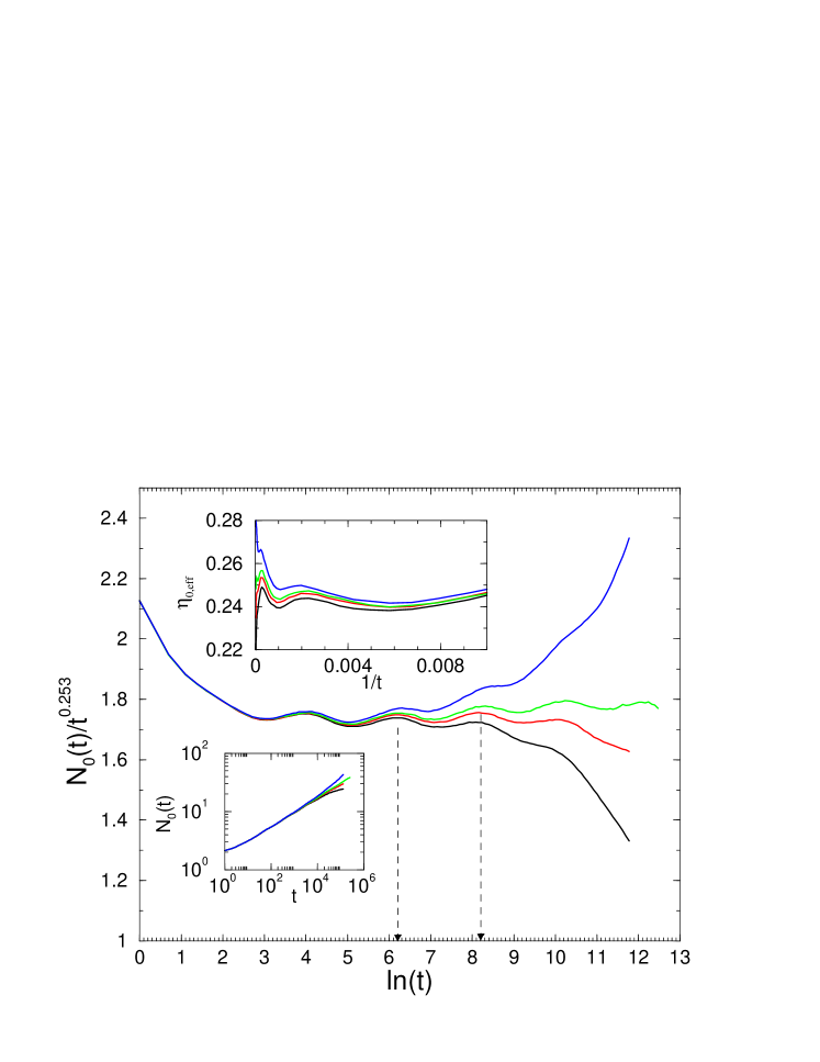
Figure 4: Time-dependence of the particle number $N_{0}(t)$ in the $k=1$ Fibonacci network for $\lambda=3.013,3.014,3.0145,3.016$ (from bottom to top). Log-periodic modulations at criticality with a period $\ln\tau=2.0(1)$ can be read-off. The upper inset shows the corresponding local slopes; the lower inset shows the unscaled data.

The critical point estimated by the local slopes is at $\lambda=3.0146(2)$ with moderate corrections to scaling. The survival probability $P(t)$ and the $R^{2}(t)$ also show these periodic modulations with the same period $\ln\tau=2.0(1)$. This is in agreement with the expectations for critical systems with discrete spatial scale invariance. Such systems remain self-similar when lengths are rescaled by a given (non-arbitrary) scale factor $b$ that is characteristic for the system. The time-dependent quantities in such models are expected to display log-periodic oscillations with a temporal period $\ln\tau$ that is related to the spatial scale factor through

$$\ln\tau=z\ln b,$$ (9)

where $z$ is the dynamical exponent of the model bab . The numerical values of the spatial scale factors $b$ of the networks under study juhasz ; boettcher and the estimated temporal periods are given in Table I and II. The data are in satisfactory agreement with Eq. (9).

As aforementioned, we performed simulations with three different positions of the initial active seed. According to the numerical results (see Table I and II), in the three cases the exponents $\eta_{m}$ and $\delta_{m}$ are different, whereas $z_{m}$ and the sum $\eta_{m}+\delta_{m}$ are independent of the initial position $m$ . The latter means that the growth rate of the number of active sites averaged in surviving samples, i.e. $N_{m}(t)/P_{m}(t)$, is not influenced by the location $m$ of the initial seed.

As opposed to this, the survival probability is sensitive to this circumstance. We have found that $\delta_{0}>\delta_{l}$, which is intuitively obvious and can be explained as follows. The survival probability is greatly influenced by the relative position of the growing cluster with respect to the long edges as the active region reaches them. If the process starts from the central site, the cluster grows typically symmetrically around the central site. Since the longer edges are also located symmetrically around the central site, the growing cluster overlaps with itself as in a finite system with periodic boundary conditions. This, however, decreases the survival probability because the rate of unsuccessful activation attempts is higher in an overlapping front. Thus in this case, the long edges of the network are not utilized in a favorable way from the point of view of the survival of the process. Apparently, for initial sites which have an environment identical to that of the central one but only within a finite radius, the growth is described by the same exponents until the cluster is within this radius.

Contrary to this, when the process is started at a site with a long edge, the infection is transferred immediately to a far away place and the two clusters spreading out from the two sites connected by the long edge do not hinder each other. Of course, in case of a long edge of length $l$, the two advancing fronts meet after time $t\sim O(l^{z})$ and the exponents $\eta_{l}$ and $\delta_{l}$ describe the spreading dynamics only below this time scale. At this time scale, a crossover occurs to a region with a faster decaying survival probability. In fact, for a typical initial seed location, the dynamical quantities suffer a series of crossovers, depending on the relative position of the initial site with respect to the longer and longer edges the cluster hits.

On the grounds of the above argumentations, the most favorable initial site for the cluster survival is the site at the longest edge, while, disregarding the surface site, the most unfavorable site is the central one. Therefore, the decay of the average survival probability must be bounded by the surviving probabilities in the above two extremal situations and we expect $\delta_{0}\geq\delta_{av}\geq\delta_{l}$ to hold. According to our numerical results, these relations are valid indeed.

Starting from a fully occupied initial state, the decay of the density at the critical point is characterized by the exponent $\alpha$ as shown in Fig.5.

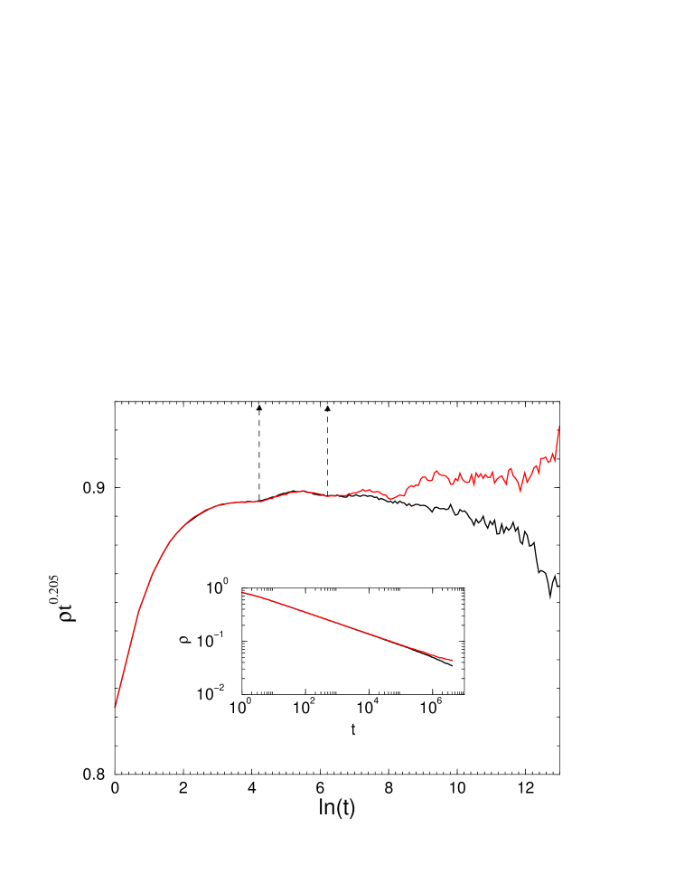
Figure 5: Density decay in the $k=1$ Fibonacci network for $\lambda=3.0145,3.016$ (from bottom to top). Log-periodic oscillations can be seen as for $N_{0}(t)$. The inset shows the unscaled data.

As can be seen from the estimated exponents given in the tables, in general, $\delta_{m}\neq\alpha$, in contrast with the CP on regular lattices, where $\delta=\alpha$ holds. As a consequence, the hyper-scaling law of DP does not hold on the networks under study, i.e. $2\delta_{m}+\eta_{m}\neq d/z$ with $d=1$. But the set of critical exponents are compatible with the generalized hyper-scaling-law TTP :

$$\delta_{m}+\alpha+\eta_{m}=d/z\ .$$ (10)

with $d=1$. We thus conclude that the rapidity reversal symmetry, which is necessary to the validity of the hyper-scaling law is broken. In other words, $P(t)$ and $\rho(t)$ scale in a different way, which is a consequence of the presence of long edges that render the system inhomogeneous in space. The inhomogeneity of the system is illustrated in Fig. 6, where the local particle densities $\langle n_{l}(t)\rangle$ are plotted at different times against the distance $l$ measured from the center. As can be seen, the regularly arranged long edges induce modulations in the profiles. As the number of infected sites grows at criticality as given in Eq. 4 and the active sites are concentrated in a region of size $\xi(t)\sim t^{1/z}$, we expect the density profiles to have the following scaling form:

$$\langle n_{l}(t)\rangle=t^{\eta_{m}-1/z}\tilde{\rho}(l/t^{1/z}).$$ (11)

This has been plotted in Fig. 6. As can be seen, the number of peaks in the profiles is increasing with $t$ and, as a consequence, the scaling function $\tilde{\rho}(x)$ is non-smooth.

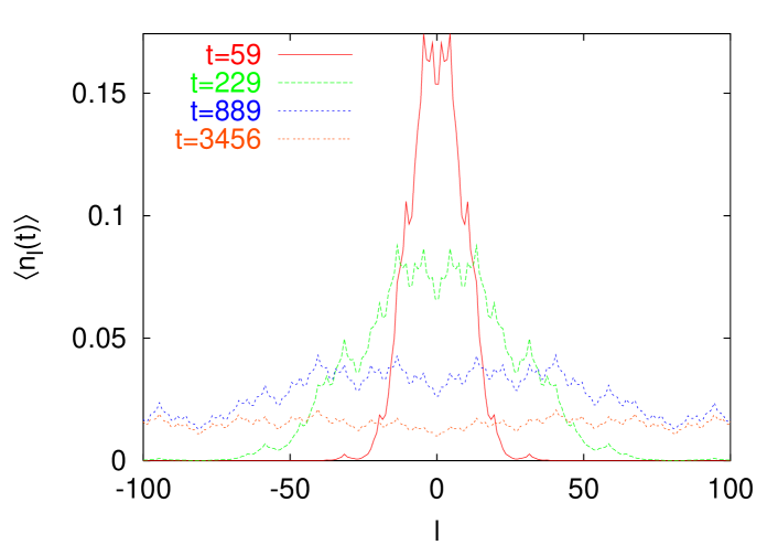
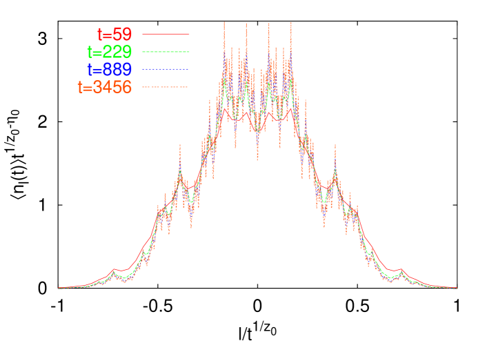
Figure 6: Upper figure: Average occupation numbers $\langle n_{l}(t)\rangle$ of sites at different times, plotted against the distance $l$ measured from the center. The logarithms of times are integer multiples of the estimated temporal period $\ln\tau$. The process was started from the central sites of the $k=1$ tripling network and the averaging has been performed over $10^{7}$ runs. Lower figure: Scaling plot with the same data.

Nevertheless, the numerical results suggest that $\delta_{av}=\alpha$ is valid within error margin, thus for the average cluster-spreading exponents the hyper-scaling of DP is fulfilled, i.e.

$$2\delta_{av}+\eta_{av}=1/z.$$ (12)

This indicates that the breaking of rapidity reversal symmetry is indeed related to the presence of the spatial inhomogeneities in the system. This is in agreement with field theory of directed percolation with long-range spreading JS08 , where the rapidity reversal symmetry persists.

Similar to the $k=1$ Fibonacci network, we performed the above analysis for the $k=1,2$ silver-mean and tripling networks and for the $k=2$ Hanoi-tower network (see Figs. 7,8 and 9). The contact process on these networks exhibits the same qualitative features as on the $k=1$ Fibonacci network except that, for the Hanoi-tower network, log-periodic oscillations cannot be observed presumably owing to their small amplitude. The estimates of critical exponents, which depend on the underlying network, can be found in Table I and II.

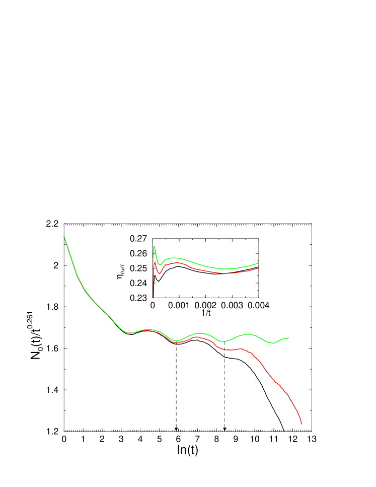
Figure 7: Time-dependence of the particle number $N_{0}(t)$ in the $k=1$ silver-mean network for $\lambda=3.081,3.082,3.083$ (from bottom to top). The period of oscillations is $\ln\tau=2.5(1)$. The inset shows the effective exponents.

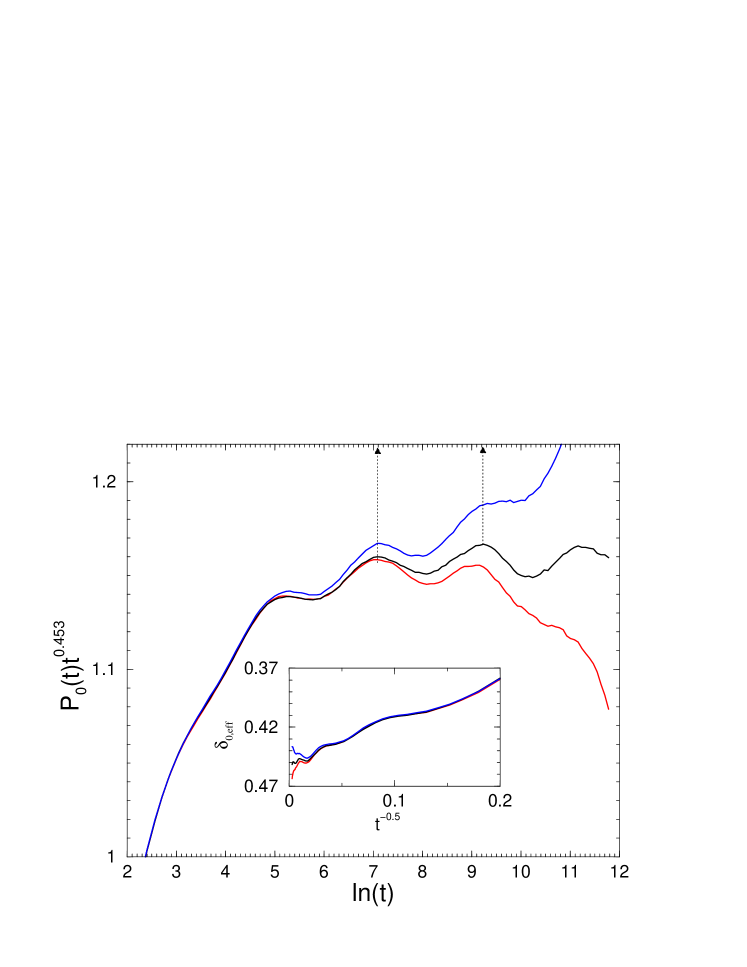
Figure 8: Time-dependence of the survival probability $P_{0}(t)$ in the $k=2$ silver-mean network for $\lambda=2.2896,2.28979,2.29$ (from bottom to top). The period of oscillations is $\ln\tau=2.1(1)$. The inset shows the effective exponents.

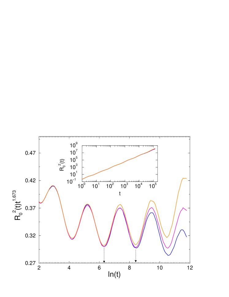
Figure 9: Time-dependence of the spread $R^{2}_{0}(t)$ in the $k=2$ silver-mean network for $\lambda=2.2896,2.28979,2.29$ (from bottom to top). The inset shows the unscaled data.

V Discussion

First, we give a brief summary of the results obtained so far. In each network, a phase transition between active and inactive phases can be identified at some finite value of the control parameter by inspecting dynamical properties such as the time dependence of the number of active sites, the survival probability and the spread. At the absorbing phase transition, conventional power-law dependence of the above quantities can be observed apart from log-periodic oscillations that are related to the discrete scale invariance of the underlying networks. In a given network, the critical exponents $\eta_{m}$ and $\delta_{m}$ depend on the location of the initial seed. The cluster exponents satisfy the generalized hyper-scaling relation. However, in case of averaging over runs started at different initial seed coordinates, the hyper-scaling relation of DP holds, too. This means that the rapidity reversal symmetry is broken as a consequence of the spatial inhomogeneity. The dynamical critical exponents of the phase transition differ from that of the one-dimensional DP universality class and are found to be characteristic for the underlying network.

We close this work by discussing the relation between the critical exponents of the CP and the shortest-path dimension (or random-walk dimension) of the underlying network. The measured critical exponents of the six network models are plotted against the random-walk dimension of the corresponding network in Fig. 10.

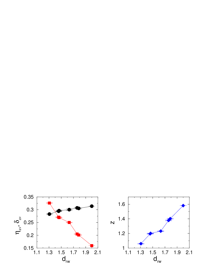
Figure 10: The critical exponents $\eta_{av}$ ($\bullet$), $\delta_{av}=\alpha$ ($\blacksquare$) and $z$ ($\blacklozenge$) of the six studied systems and the one-dimensional CP plotted against $d_{\rm rw}$ of the underlying network.

For decreasing $d_{\rm rw}$ the critical exponents $\eta_{av}$ and $\delta_{av}=\alpha$ move towards the mean-field values of DP ($\eta_{MF}=0$, $\delta_{MF}=1$) almost monotonically. These exponents lie in between the corresponding values of the one-dimensional and the two-dimensional DP universality classes. Contrary to this, the dynamical exponent $z$ does not move toward the mean field value $z_{MF}=2$, but decreases with decreasing $d_{\rm rw}$. Thus, it moves parallel with the dynamical exponent of the random walk.

We recall that the $k=1$ silver mean and $k=1$ Fibonacci network are the first two members of a family of networks, which are defined by the inflation rule in Eq. (1), and which are parameterized by an integer $n$. For these networks, it is known that $d_{\rm min}\to 1$ and $d_{\rm rw}\to 2$ when $n\to\infty$, i.e. in this limit, the characteristics of the regular one-dimensional lattice are recovered juhasz . Therefore, we conjecture that the critical exponents of CP defined on these networks approach the one-dimensional DP values without limits as $n\to\infty$. In the opposite limit, i.e. when $d_{\rm rw}\to 1$ (and $d_{\rm min}\to 0$), it is an open question what are the limiting values of the critical exponents of the CP.

Finally, we mention that the above observations open up the possibility to design networks on which dynamical processes evolve in a prescribed way. The optimization of spreading or transport processes in networks is of great practical relevance kleinberg ; mcculloh ; PSV . Besides the tuning of degree-distribution or the dependence of transition rates on the degrees of sites in non-regular (such as scale-free) networks giuraniuc ; kji ; yang , the networks studied in this work offer an alternative way of controlling critical dynamics by means of choosing appropriate sets of long links and the findings obtained here may provide ideas in optimization problems.

- (1) G. Ódor, Universality in Nonequilibrium Lattice Systems, World Scientific, 2008; Rev. Mod. Phys. 76, 663 (2004).
- (2) T. E. Harris, Ann. Prob., 2, 969 (1974).
- (3) P. Grassberger and A. de la Torre, Ann. Phys. 122, 373 (1979).
- (4) H. K. Janssen, Z. Phys. B 42, 151 (1981).
- (5) P. Grassberger, Z. Phys. B 47, 365 (1982).
- (6) J. Marro and R. Dickman, Nonequilibrium phase transitions in lattice models, Cambridge University Press, Cambridge 1999.
- (7) M. Henkel, H. Hinrichsen and S. Lübeck, Nonequilibrium Phase Transitions, Springer Berlin (2008).
- (8) H. Hinrichsen, J. Stat. Mech.: Theor. Exp. P07006 (2007).
- (9) R. Pastor-Satorras and A. Vespignani, Phys. Rev. Lett. 86, 3200 (2001); Phys. Rev. E 63, 066117 (2001); C. Castellano and R. Pastor-Satorras, Phys. Rev. Lett. 96, 038701 (2006); Phys. Rev. Lett. 98, 029802 (2007); Phys. Rev. Lett. 100, 148701 (2008); M. Ha, H. Hong, and H. Park, Phys. Rev. Lett. 98, 029801 (2007).
- (10) For a review, see: S. N. Dorogovtsev, A. V. Goltsev, J. F. F. Mendes, Rev. Mod. Phys. 80, 1275 (2008).
- (11) R. Albert, A.-L. Barabási, Rev. Mod. Phys. 74, 47-97 (2002).
- (12) D. Chowdhury and B. Chakrabarti, J. Phys. A: Math. Gen. 18, L377 (1985).
- (13) M.E.J. Newman and D.J. Watts, Phys. Lett. A 263, 341 (1999).
- (14) C.F. Moukarzel, Phys. Rev. E 60, R6263 (1999).
- (15) R. Monasson, Eur. Phys. J. B 12, 555 (1999).
- (16) S. Jespersen and A. Blumen, Phys. Rev. E 62, 6270 (2000).
- (17) I. Benjamini and N. Berger, Rand. Struct. Alg. 19, 102 (2001).
- (18) P. Sen and B. Chakrabarti, J. Phys. A: Math. Gen. 34, 7749 (2001).
- (19) C.F. Moukarzel and M. Argollo de Menezes, Phys. Rev. E 65, 056709 (2002).
- (20) D. Coppersmith, D. Gamarnik and M. Sviridenko, Rand. Struct. Alg. 21, 1 (2002).
- (21) J.M. Kleinberg, Nature 406, 845 (2000).
- (22) I. Benjamini and C. Hoffman, Electr. J. Comb., 12, R46 (2005).
- (23) S. Boettcher, B. Gonçalves and H. Guclu, J. Phys. A: Math. Theor. 41, 252001 (2008); S. Boettcher and B. Gonçalves, Europhys. Lett. 84, 30002 (2008).
- (24) R. Juhász, Phys. Rev. E 78, 066106 (2008).
- (25) D.J. Watts and S.H. Strogatz, Nature 393, 440 (1998).
- (26) P. Frojdh, M. Howard, K. B. Lauritsen, J. Mod. Phys. B 15, 1761-1797 (2001).
- (27) M. A. Bab, G. Fabricius and E. V. Albano, Eur. Phys. Lett. 81 10003 (2008).
- (28) J. F. F. Mendes, R. Dickman, M. Henkel and M. C. Marques, J. Phys. A 27, 3019 (1994).
- (29) H-K. Janssen and O. Stenull, Phys. Rev. E 78, 061117 (2008).
- (30) K. A. McCulloh, J. S. Sperry and F. R. Adler, Nature 421, 939 (2003).
- (31) R. Pastor-Satorras and A. Vespignani, Evolution and Structure of the Internet: A Statistical Physics Approach, Cambridge University Press, Cambridge (2004).
- (32) C. V. Giuraniuc, J. P. L. Hatchett, J. O. Indekeu, M. Leone, I. Pérez Castillo, B. Van Schaeybroeck and C. Vanderzande, Phys. Rev. Lett. 95, 098701 (2005); Phys. Rev. E 74, 036108 (2006).
- (33) M. Karsai, R. Juhász and F. Iglói, Phys. Rev. E 73, 036116 (2006).
- (34) R. Yang, T. Zhou, Y.-B. Xie, Y.-C. Lai and B.-H. Wang, Phys. Rev. E 78, 066109 (2008).