Wigner-function theory and decoherence of the quantum-injected optical parametric amplifier

Abstract

Recent experimental results demonstrated the generation of a quantum superpositon (MQS), involving a number of photons in excess of $5\times 10^{4}$, which showed a high resilience to losses. In order to perform a complete analysis on the effects of de-coherence on this multiphoton fields, obtained through the Quantum Injected Optical Parametric Amplifier (QIOPA), we invesigate theoretically the evolution of the Wigner functions associated to these states in lossy conditions. Recognizing the presence of negative regions in the W-representation as an evidence of non-classicality, we focus our analysis on this feature. A close comparison with the MQS based on coherent $|\alpha\rangle$ states allows to identify differences and analogies.

I Introduction

In the last decades the physical implementation of macroscopic quantum superpositions (MQS) involving a large number of particles has attracted a great deal of attention. Indeed it was generally understood that the experimental realization of a MQS is very difficult and in several instances practically impossible owing to the extremely short persistence of quantum coherence, i.e., of  the extremely rapid decoherence due to the entanglement established between the macroscopic system and the environment Niel00 ; Zure91 ; Zure03 ; Zure07 . Formally, the irreversible decay towards a probabilistic classical mixture is implied theoretically by the tracing operation of the overall MQS state over the environmental variables Dur02 ; Dur04 . In the framework of quantum information different schemes based on optical systems have been undertaken to generate and to detect the MQS condition. A Cavity - QED scheme based on the interaction between Rydberg atoms and a high-Q cavity has lead to the indirect observation of Schrödinger Cat states and of their temporal evolutions. In this case the microwave MQS field stored in the cavity can be addressed indirectly by injecting in the cavity, in a controlled way, resonant or non-resonant atoms as ad hoc ”measurement mouses” Brun92 ; Raim01 . A different approach able to generate freely propagating beams adopts photon-subtracted squeezed states; experimental implementations of quantum states with an average number of photons of around four have been reported both in the pulsed and continuous wave regimes Neer06 ; Ourj06 ; Ourj07 ; Ourj09 . These states exhibit non-gaussian characteristics and open new perspectives for quantum computing based on continuous-variable (CV) systems, entanglement distillation protocols Eise02 ; Dong08 , loophole free tests of Bell’s inequality.

In the last few years a novel ”quantum injected” optical parametric amplification (QI-OPA) process has been realized in order to establish the entanglement between a single photon and a multiphoton state given by an average of many thousands of photons, a Schrödinger Cat involving a ”macroscopic field”. Precisely, in a high-gain QI-OPA ”phase-covariant” cloning machine the multiphoton fields were generated by an optical amplifier system bearing a high nonlinear (NL) gain $g$ and seeded by a single-photon belonging to an EPR entangled pair DeMa98 ; DeMa98a ; DeMa05a ; DeMa05 ; Scia05 .

While a first theoretical insight on the dynamical features of the QIOPA macrostates and a thorough experimental characterization of the quantum correlations were recently reported Naga07 ; DeMa08 , a complete quantum phase-space analysis able to recognize the persistence of the QI-OPA properties in a decohering environment is still lacking Schl01 ; Wign32 . Among the different representation of quantum states in the continuous-variables space Cahi69 , the Wigner quasi-probability representation has been widely exploited as an evidence of non-classical properties, such as squeezing Wall95 and EPR non-locality Bana98 . In particular, the presence of negative quasi-probability regions has been considered as a consequence of the quantum superposition of distinct physical states Bart44 .

In the present paper we investigate the Wigner functions associated to multi-photon states generated by optical parametric amplification of microscopic single photon states. We focus our interest on the effects of de-coherence on the macro-states and on the emergence of the ”classical” regime in the amplification of initially pure quantum states. The Wigner functions of these QI-OPA generated states in presence of losses are analyzed in comparison with the paradigmatic example of the superposition of coherent, Glauber’s states, $|\alpha\rangle$.

The paper is structured as follows. In Section II, we introduce the conceptual scheme and describe the evolution of the system both in the Heisenberg and Schrödinger picture. Section III is devoted to the calculation of the Wigner function of the QI-OPA amplified field. We first consider a single-mode amplifier, which is analogous to the case of photon-subtracted squeezed vacuum. Then we derive a compact expression of the Wigner function in the case of a two-mode amplifier in the ”collinear” case, i.e. for common $k-$vectors of the amplified output fields. In Section IV, we introduce, for the collinear case, a decoherence model apt to simulate the de-cohering losses affecting the evolution of the macrostates density matrix. This evolution is then compared to the case of the coherent $|\alpha\rangle$ MQS. Section V is devoted to a brief review of the features of coherent states superpositions (CSS). Hence in Section VI we derive an explicit analytic expression of the Wigner functions for the QI-OPA amplified states in presence of decoherence. The negative value of the W-representation in the origin of the phase-space for such states above a certain value of the ”system-enviroment ” interaction parameter, is an evidence of the persistance of quantum properties in presence of decoherence. This aspect is then compared with the case of the $|\alpha\rangle$ states superposition. Then in Section VII we study a complementary approach to enlighten the resilience to losses of the QI-OPA MQS with respect to the $|\alpha\rangle$ states superposition. Precisely, we define a coherence parameter, based on the concept of state-distance in Hilbert spaces, and we study its decrease as a function of the losses parameter for both classes of MQS. Finally, in Section VIII we analyze a different configuration based on a non-collinear optical parametric amplifier in the quantum injected regime, i.e. a universal quantum cloning machine. We calculate the Wigner function associated to the states generated by this device in absence and in presence of decoherence, focusing on the persistence of quantum properties after the propagation over a lossy channel.

II Optical parametric amplification of a single photon state

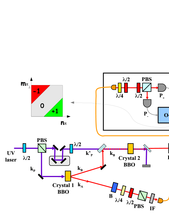
Figure 1: Scheme of the experimental setup. The main UV laser beam provides the OPA excitation field beam at $\lambda=397.5nm$. A type II BBO (Beta Barium Borate) crystal (crystal 1: C1) generates pair of photons with $\lambda=795nm$. In virtue of the EPR non-local correlations established between the modes $\mathbf{k}_{A}$ and $\mathbf{k}_{B}$, the preparation of a single-photon on mode $\mathbf{k}_{B}$ with polarization state $\vec{\pi}_{\varphi}$ is conditionally determined by detecting a single-photon after proper polarization analysis on the mode $\mathbf{k}_{A}$ (polarizing beamsplitter (PBS), $\lambda/2$ and $\lambda/4$ waveplates, Soleil-Babinet compensator (B), interferential filter (IF)). The photon belonging to $\mathbf{k}_{B}$, together with the pump laser beam $\mathbf{k}_{p}^{\prime}$, is fed into an high gain optical parametric amplifier consisting of a NL crystal 2 (C2), cut for collinear type-II phase matching. The fields are coupled to single-mode fibers. For more details refer to DeMa08 . Right Inset: Measurement apparatus. After fiber polarization compensation, the field is analyzed by two photomultipliers $\left\{P_{+},P_{-}\right\}$ and then discriminated through an O-Filter device. Left inset: Action of the O-Filter in the photon number space: the ($\pm 1$) outcomes are assigned whether $n_{\pi}-m_{\pi_{\bot}}>k$ or $m_{\pi_{\bot}}-n_{\pi}>k$, where $k$ is a tunable threshold condition. The central region leads to an inconclusive (0) outcome, and the two orthogonal macrostates cannot be discriminated.

As a first step we consider the generation of a multiphoton quantum field, obtained by parametric amplification. Let us briefly describe the conceptual scheme. An entangled pair of two photons in the singlet state $\left|\psi^{-}\right\rangle_{A,B}$=$2^{-{\frac{1}{2}}}\left(\left|H\right\rangle_{A}\left|V\right\rangle_{B}-\left|V\right\rangle_{A}\left|H\right\rangle_{B}\right)\$is produced through a spontaneous parametric down-conversion (SPDC) by crystal 1 pumped by a pulsed UV pump beam: Fig.1. There $\left|H\right\rangle$ and $\left|V\right\rangle$ stands, respectively, for a single photon with horizontal and vertical polarization $(\overrightarrow{\pi})$ while the labels $A,B$ refer to particles associated respectively with the spatial modes $\mathbf{k}_{A}$and $\mathbf{k}_{B}$. The photon belonging to $\mathbf{k}_{B}$, together with a strong UV pump beam, is fed into an optical parametric amplifier consisting of a non-linear crystal 2 pumped by the beam $\mathbf{k}_{P}^{\prime}$. The crystal 2 is oriented for ”collinear operation”, i.e., emitting pairs of amplified photons over the same spatial mode which supports two orthogonal $\overrightarrow{\pi}$ modes, respectively horizontal and vertical. Let us analyze the properties of the resultant amplified field.

II.1 Collinear optical parametric amplifier

The complete Hamiltonian of the system reads:

$$\hat{\mathcal{H}}=\hbar\omega\left(\hat{a}_{H}^{\dagger}\hat{a}_{H}+\hat{a}_{V}^{\dagger}\hat{a}_{V}\right)+i\hbar\chi\left(\hat{a}_{H}^{\dagger}\hat{a}_{V}^{\dagger}e^{-2i\omega t}-\hat{a}_{H}\hat{a}_{V}e^{2i\omega t}\right)$$ (1)

where $\chi$ is proportional to the 2^nd order non-linear susceptibility and to the amplitude of the pump field $E_{0}^{P}$; $\hat{a}_{H}^{\dagger}$ and $\hat{a}_{V}^{\dagger}$ are the creation operators associated to the mode $\mathbf{k}$ respectively, with polarization $\overrightarrow{\pi}$ horizontal and vertical, ${H,V}$. We assume a classical and undepleted coherent pump field. Let us consider only the interaction contribution to $\hat{\mathcal{H}}$ and a reference system which rotates with angular speed $2\omega$. The time-independent interaction Hamiltonian is found to be:

$$\hat{\mathcal{H}}_{I}=i\hbar\chi\left(\hat{a}_{H}^{\dagger}\hat{a}_{V}^{\dagger}-\hat{a}_{H}\hat{a}_{V}\right)$$ (2)

The Heisenberg evolution equations are:

$$\frac{\partial\hat{a}_{\pi}}{\partial t}=\frac{1}{i\hbar}\left[\hat{a}_{\pi},\hat{\mathcal{H}}_{I}\right]=\chi\hat{a}_{\pi^{\perp}}^{\dagger}$$ (3)

with general solution:

$$\hat{a}_{\pi}\left(t\right)=\hat{a}_{\pi}\left(0\right)\cosh\left(\chi t\right)+\hat{a}_{\pi^{\perp}}^{\dagger}\left(0\right)\sinh\left(\chi t\right)$$ (4)

where $\pi={H,V}$.

The average number of photons generated in the SPDC process can be easily calculated in the Heisenberg picture formalism by applying the evoluted operators to the initial vacuum state $|0H,0V\rangle\equiv|0\rangle$. Heretofore, $|n\pi,m\pi_{\bot}\rangle$ stands for the Fock-state with $n$ photons with $\pi$ polarization and $m$ photons with the orthogonal $\pi_{\bot}$ one. For the horizontal polarization we get:

$$\langle 0|\hat{a}_{H}^{\dagger}\left(t\right)\hat{a}_{H}\left(t\right)|0\rangle=\sinh^{2}\left(\chi t\right)\equiv\overline{m}$$ (5)

The same result holds for the vertical polarization.

II.2 Output wavefunctions

In any ”equatorial” polarization basis $\{\left|\varphi\right\rangle,\left|\varphi^{\perp}\right\rangle\}$, referred to a Poincaré sphere with ”poles” $\left|H\right\rangle$ and $\left|V\right\rangle$, the Hamiltonian of the polarization non-degenerate optical parametric amplifier, described by the expression (2), can be expressed as:

$$\hat{\mathcal{H}}_{I}=i\hbar\frac{\chi}{2}e^{-\imath\varphi}\left((\hat{a}_{\varphi}^{\dagger})^{2}-e^{\imath 2\varphi}(\hat{a}_{\varphi\perp}^{\dagger})^{2}\right)+h.c.$$ (6)

where the corresponding field operators are: $\hat{a}_{\varphi}^{\dagger}=\frac{1}{\sqrt{2}}\left(\hat{a}_{H}^{\dagger}+e^{i\varphi}\hat{a}_{V}^{\dagger}\right)$, $\hat{a}_{\varphi\perp}^{\dagger}=\frac{1}{\sqrt{2}}\left(\hat{a}_{H}^{\dagger}-e^{i\varphi}\hat{a}_{V}^{\dagger}\right)$.

The Hamiltonian can then be separated in the two polarization components $\{\vec{\pi}_{\varphi},\vec{\pi}_{\varphi^{\perp}}\}$. The time-dependent field operators are:

$$\hat{a}_{\varphi}(t)=\hat{a}_{\varphi}(0)\cosh(\chi t)+e^{-\imath\varphi}a_{\varphi}^{\dagger}(0)\sinh(\chi t)$$ (7)

Let us now restrict the analysis to the basis $\left\{\vec{\pi}_{+},\vec{\pi}_{-}\right\}$, in which we calculate the output wavefunction in the Schroedinger picture; the unitary evolution operator is

$$\hat{U}=\exp\left(-i\frac{\hat{\mathcal{H}}_{I}t}{\hbar}\right)=\hat{U}_{+}\hat{U}_{-}$$ (8)

with

$$\hat{U}_{\pm}=\exp[\pm\frac{g}{2}\left(\hat{a}_{\pm}^{\dagger 2}-\hat{a}_{\pm}^{2}\right)]$$ (9)

where $g=\chi t$ is the non linear gain of the process.

The expression of $\hat{U}$ enlightens the decoupling between the two polarization modes. A simple expression of the operators $\hat{U}_{+}$ and $\hat{U}_{-}$ can be obtained adopting the following operatorial relation Coll88 :

$$\hat{U}_{\pm} = \exp\left[\pm\Gamma\left(\frac{\hat{a}_{\pm}^{\dagger}}{\sqrt{2}}\right)^{2}\right]\exp\left[-\ln(\cosh g)\left(\hat{a}_{\pm}^{\dagger}\widehat{a}_{\pm}+\frac{1}{2}\right)\right]\times$$ (10)

$$\times\exp\left[\mp\Gamma\left(\frac{\hat{a}_{\pm}}{\sqrt{2}}\right)^{2}\right]$$

with $\Gamma=\tanh g$. Let us consider the injection of a single photon state with generic equatorial polarization $\vec{\pi}_{\varphi}$ into the OPA:

$$\left|\psi_{in}\right\rangle = |\varphi\rangle=\frac{1}{\sqrt{2}}\left(\left|H\right\rangle+e^{i\varphi}\left|V\right\rangle\right)=$$ (11)

$$= e^{i\frac{\varphi}{2}}\left(\cos\frac{\varphi}{2}\left|1+,0-\right\rangle+i\sin\frac{\varphi}{2}\left|0+,1-\right\rangle\right)$$

The multiphoton output state of the amplifier is found:

$$\left|\Psi_{out}\right\rangle=|\Phi^{\varphi}\rangle=\cos\frac{\varphi}{2}\left|\Phi^{+}\right\rangle+i\sin\frac{\varphi}{2}\left|\Phi^{-}\right\rangle$$ (12)

where:

$$\left|\Phi^{\pm}\right\rangle=\hat{U}_{\pm}\hat{U}_{\mp}\left|1\pm,0\mp\right\rangle=\left(\hat{U}_{\pm}\left|1\right\rangle_{\pm}\right)\left(\hat{U}_{\mp}\left|0\right\rangle_{\mp}\right)$$ (13)

Simple calculations lead to the expressions:

$$\left|\Phi^{\pm}\right\rangle=\frac{1}{C^{2}}\sum_{i,j}\left(-\frac{\Gamma}{2}\right)^{j}\left(\frac{\Gamma}{2}\right)^{i}\frac{\sqrt{2j!}}{j!}\frac{\sqrt{(2i+1)!}}{i!}\left|(2i+1)\pm,2j\mp\right\rangle$$ (14)

where $C=\cosh g$. The quantum states $\left|\Phi^{+}\right\rangle$ and $\left|\Phi^{-}\right\rangle$ are orthogonal, being the unitary evolution of initial orthogonal states. We observe that $\left|\Phi^{+}\right\rangle$ presents an odd number of $\vec{\pi}_{+}$ polarized photons and an even number of $\vec{\pi}_{-}$ polarized ones. Conversely for $\left|\Phi^{-}\right\rangle$.

The average number of photons with polarization $\vec{\pi}_{+}$ can be estimated in the Heisenberg representation as:

$$\left\langle\hat{n}_{+}\right\rangle=\left\langle\psi_{in}\right|\hat{a}_{+}^{\dagger}(t)\hat{a}_{+}(t)\left|\psi_{in}\right\rangle=\bar{m}+\left(2\bar{m}+1\right)\cos^{2}\left(\frac{\varphi}{2}\right)$$ (15)

where $\bar{m}=\sinh^{2}\left(g\right)$. The phase dependence shows that for $\varphi=\pi$ the average number of generated photons is equal to the spontaneous one, while for $\varphi=0$, corresponding to the stimulated case, an increase of a factor $3$ is observed in the average number of $\vec{\pi}_{+}$ polarized photons.

Likewise, the average number of photons $\vec{\pi}_{-}$ polarized is given by:

$$\left\langle\hat{n}_{-}\right\rangle=\left\langle\psi_{in}\right|\hat{a}_{-}^{\dagger}(t)\hat{a}_{-}(t)\left|\psi_{in}\right\rangle=\bar{m}+\left(2\bar{m}+1\right)\sin^{2}(\frac{\varphi}{2})$$ (16)

Hence, by varying the phase $\varphi$ we observe a fringe pattern which exhibits a gain dependent visibility:

$$\emph{V}_{th}^{(1)}=\frac{\left\langle n_{+}\left(\varphi=0\right)\right\rangle-\left\langle n_{-}\left(\varphi=0\right)\right\rangle}{\left\langle n_{+}\left(\varphi=0\right)\right\rangle+\left\langle n_{-}\left(\varphi=0\right)\right\rangle}=\frac{2\bar{m}+1}{4\bar{m}+1}$$ (17)

In the asymptotic limit ($g\rightarrow\infty$) $\emph{V}_{th}^{(1)}=\frac{1}{2}$.

We now briefly discuss the phase-covariance properties of the optical parametric amplifier when injected by a single-photon state. In this configuration, this device acts as optimal phase-covariant cloning machines, and due to the unitary evolution of the process, the superposition character of any generic input state $|\varphi\rangle=\frac{1}{\sqrt{2}}\left(|H\rangle+e^{\imath\varphi}|V\rangle\right)$ is maintained after the amplification:

$$|\Phi^{\varphi}\rangle=\frac{1}{\sqrt{2}}\left(|\Phi^{H}\rangle+e^{\imath\varphi}|\Phi^{V}\rangle\right)$$ (18)

Let us stress that there is freedom in the choice of the macrostates basis vectors. For example, the $|\Phi^{\pm}\rangle$ states can be used in the expansion of the overall state as in (12). Hence, the equatorial $|\Phi^{\varphi}\rangle$ amplified state can be written as the macroscopic quantum superposition either of the $\left\{|\Phi^{+}\rangle,|\Phi^{-}\rangle\right\}$ and the $\left\{|\Phi^{H}\rangle,|\Phi^{V}\rangle\right\}$ ”basis” states. Furthermore, due to their resilience to decoherence DeMa09 , all equatorial macro-qubits represent a preferred ”pointer states basis” Zure03 for writing $|\Phi^{\varphi}\rangle$ in the form of a macroscopic quantum superposition.

III Wigner functions of the amplified field

In order to investigate the properties of the output field of the QI-OPA device in more details, we analyze the quasi-probability distribution introduced by Wigner Wign32 for the amplified field. The Wigner function is defined as the Fourier transform of the symmetrically-ordered characteristic function $\chi(\eta)$ of the state described by the general density matrix $\hat{\rho}$

$$\chi(\eta)=Tr\left[\hat{\rho}\exp\left(\eta\hat{a}^{\dagger}-\eta^{\ast}\hat{a}\right)\right]$$ (19)

The associated Wigner function

$$W(\alpha)=\frac{1}{\pi^{2}}\int\exp\left(\eta^{\ast}\alpha-\eta\alpha^{\ast}\right)\chi\left(\eta\right)d^{2}\eta$$ (20)

exists for any $\hat{\rho}$ but is not always positive definite and, consequently, can not be considered as a genuine probability distribution. Since the early decades of quantum mechanics, the emergence of negative probabilities has been identified as a peculiar feature of quantum physics, and has been connected to the mathematical segregation of states which physically live only in combination Bart44 . In parallel, the non classicality of a quantum state is expressed by a Glauber’s P-representation Glau63 ; Suda63 ; Cahi69 which is more singular than a delta function, i.e. the $P(\alpha)$ proper of coherent states. This means that the system does not possess an expansion, in terms of the overcomplete semi-classical $|\alpha\rangle$ state basis, that can be interpreted as a probability distribution. However, the negativity of the Wigner function is not the only parameter that allows to estimate the non-classicality of a certain state. For example, the squeezed vacuum state Wall95 presents a positive $W$-representation, while its properties cannot be described by the laws of classical physics. Furthermore, recent papers have shown that the Wigner function of an EPR state provides direct evidence of its non-local character Cohe97 ; Bana98 , while being completely-positive in all the phase-space.

The complex variable $\alpha$ in (20) is the eigenvalue associated to the non-Hermitian operator $\hat{a}$ which acts upon the coherent state $|\alpha\rangle$ as follows: $\hat{a}|\alpha\rangle=\alpha|\alpha\rangle$. It is possible to decompose $\alpha$ in its real and imaginary part and then to define the quadratures operators $\hat{X}$ and $\hat{Y}$ which allow the representation of the field in the phase space $\hat{a}=\frac{\hat{X}+i\hat{Y}}{2}$. The quadratures operators are Hermitian operators and thus correspond to physical observables proportional to the position $\hat{q}$ and the momentum $\hat{p}$ following the relations: $\hat{X}=\sqrt{\frac{2\omega}{\hbar}}\hat{q}$ and $\hat{Y}=-\sqrt{\frac{2}{\hbar\omega}}\hat{p}.$ The uncertainty principle leads to: $\Delta\hat{X}\Delta\hat{Y}\geq 1$.

III.1 Single mode amplifier

For the sake of simplicity, let us first consider the Hamiltonian of a degenerate amplifier acting on a single $k-$mode with polarization $\vec{\pi}_{+}$:

$$\hat{\mathcal{H}}_{I}=i\hbar\frac{\chi}{2}\left(\hat{a}_{+}^{\dagger 2}-\hat{a}_{+}^{2}\right)$$ (21)

When no seed is injected, the amplifier operates in the regime of spontaneous emission and the characteristic function reads:

$$\chi_{0}(\eta,t) = \left\langle 0\right|\exp[\eta\hat{a}_{+}^{\dagger}(t)-\eta^{\ast}\hat{a}_{+}(t)]\left|0\right\rangle=$$ (22)

$$= \left\langle 0\right|\exp[\eta(t)\hat{a}_{+}^{\dagger}-\eta^{\ast}(t)\hat{a}_{+}]\left|0\right\rangle$$

with $\hat{a}_{+}(t)=\hat{a}_{+}\cosh(g)+\hat{a}_{+}^{\dagger}\sinh(g)$, $\eta(t)=\eta\cosh(g)-\eta^{\ast}\sinh(g)$, and $g=\chi t$. Hereafter, we explicitly report the dependence of the Wigner function from the interaction time $t$. We obtain, using the operatorial relation $\exp(\hat{A}+\hat{B})=\exp{\hat{A}}\exp{\hat{B}}\exp(-1/2[\hat{A},\hat{B}])$:

$$\chi_{0}(\eta,t)=\exp\left(-\frac{1}{2}\left|\eta(t)\right|^{2}\right)$$ (23)

The calculation then proceeds as follows. Starting from the definition of the Wigner function (20), we perform the two subsequent transformations of the integration variables $d^{2}\eta\rightarrow d^{2}\eta(t)\rightarrow xdxd\varphi$, where $\eta\rightarrow\eta(t)$ has been defined previously and can be expressed as $\eta(t)=xe^{i\varphi}$. The Wigner function then reads:

$$W_{|0+\rangle}(\alpha,t) =\frac{1}{\pi^{2}}\int e^{x\left[\left(\bar{\alpha}-\bar{\alpha}^{\ast}\right)\cos\varphi+i\left(-\bar{\alpha}-\bar{\alpha}^{\ast}\right)\sin\varphi\right]-\frac{1}{2}x^{2}}xdxd\varphi$$ (24)

$$=\frac{2}{\pi}\int_{0}^{\infty}J_{0}\left(-2\left|\bar{\alpha}\right|x\right)\exp\left(-\frac{1}{2}x^{2}\right)xdx=$$

$$=\frac{2}{\pi}\exp\left[-2\left|\bar{\alpha}\right|^{2}\right]$$

where $\bar{\alpha}=\alpha\cosh(g)-\alpha^{\ast}\sinh(g)$, and $J_{0}(x)$ is the Bessel function of order 0. We can now write $\bar{\alpha}=\mathrm{Re}(\alpha)e^{-g}+i\mathrm{Im}(\alpha)e^{g}$ as a function of the $X$, $Y$ quadrature operators, defined by the expression $\alpha=X+iY$. By substituting such variables Eq.(24) becomes

$$W_{|0+\rangle}(X,Y,t)=\frac{2}{\pi}\exp\left[-2\left(X^{2}e^{-2g}+Y^{2}e^{2g}\right)\right]$$ (25)

When we consider the case in which a single photon with polarization $\vec{\pi}_{+}$ is injected: $\left|\psi_{in}\right\rangle=\left|1+\right\rangle$, analogous calculations leads to the characteristic function

$$\chi_{1}(\eta,t) = \left\langle 1\right|\exp[\eta(t)\hat{a}_{+}^{\dagger}-\eta^{\ast}(t)\hat{a}_{+}]\left|1\right\rangle=$$ (26)

$$= \left(1-\left|\eta(t)\right|^{2}\right)\exp\left(-\frac{1}{2}\left|\eta(t)\right|^{2}\right)$$

The Wigner function reads:

$$W_{|1+\rangle}(X,Y,t) = -\frac{2}{\pi}\left[1-4\left|\bar{\alpha}\right|^{2}\right]\exp\left[-2\left|\bar{\alpha}\right|^{2}\right]=$$ (27)

$$= -\frac{2}{\pi}\left[1-4\left(X^{2}e^{-2g}+Y^{2}e^{2g}\right)\right]\times$$

$$\times\exp\left[-2(X^{2}e^{-2g}+Y^{2}e^{2g})\right]$$

As a further example, we consider the injection of the 2-photon state $\left|\psi_{in}\right\rangle=\left|2+\right\rangle$. We obtain

$$\chi_{2}(\eta,t)=\left(1-2\left|\eta(t)\right|^{2}+\frac{1}{2}\left|\eta(t)\right|^{4}\right)\exp\left(-\frac{1}{2}\left|\eta(t)\right|^{2}\right)$$ (28)

and the Wigner function reads:

$$W_{|2+\rangle}(X,Y,t)=\frac{2}{\pi}\left[1-8\left(X^{2}e^{-2g}+Y^{2}e^{2g}\right)\right.$$

$$\left.+2\left(X^{2}e^{-2g}+Y^{2}e^{2g}\right)^{2}\right]\exp\left[-2(X^{2}e^{-2g}+Y^{2}e^{2g})\right]$$

As in the single photon case, the negativity of the Wigner function is maintained after the amplification process, emphasizing the quantum properties of the injected field. All these features are shown in Figs. 2 and 3, which report respectively the plots of the Wigner functions and of their sections $X=0$ and $Y=0$ for QI-OPA amplified states, with the injection of the $|0\rangle,|1\rangle,|2\rangle$ Fock states. The analysis of these figures shows that the amplification effect leads to the increase of the degree of squeezing for the multi-photon output field. The uncertainty on one of the two quadratures is decreased while the other one is increased coherently with the Heisenberg uncertainty principle. Let us note that the quantum character of the Fock states is underlined by the negativity of the Wigner function in the central region of the quadratures space.

Finally, this result can be generalized by analogous calculation to the generic $|N+\rangle$ input state, leading to the Wigner function:

$$W_{|N+\rangle}(\alpha,t)=\frac{2}{\pi}(-1)^{N}L_{N}\left(4|\overline{\alpha}|^{2}\right)e^{-2|\overline{\alpha}|^{2}}$$ (29)

where $L_{N}$ are Laguerre polynomials of order $N$. For all $N$, the non-classical properties of the injected state are maintained after the amplification process, as the OPA is described by a unitary evolution operator.

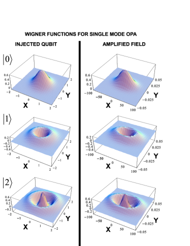
Figure 2: Wigner function of the injected states and the corresponding amplified states, for a single mode degenerate amplifier with gain $g=4$. The axes report the quadratures values $X$ and $Y$. $\left|0\right\rangle$ injection of the vacuum state. $\left|1\right\rangle$ injection of a single photon. $\left|2\right\rangle$ injection of two photons. The amplified field is plotted on a different scale with respect to the injected qubit one, due to the high degree of squeezing introduced by the amplification process.

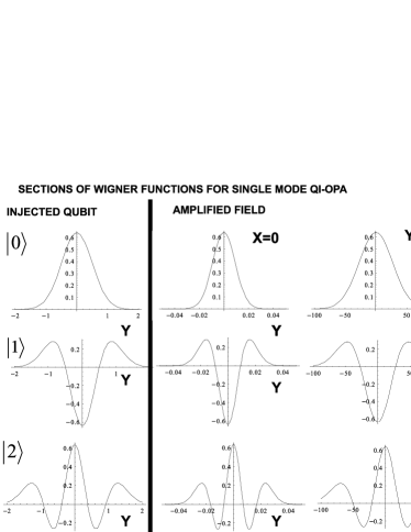
Figure 3: Sections of the input states Wigner functions and of the relatives amplified fields along the directions $X=0$ and $Y=0$. Since the injected qubit shows a rotational symmetry, we report only the $X=0$ section. $\left|0\right\rangle$ injection of the vacuum state. $\left|1\right\rangle$ injection of the single photon state. $\left|2\right\rangle$ injection of the two-photon state.

We conclude this Section on the single-mode amplifier by emphasizing the connection, shown in Bisw07 , between the single photon subtracted squeezed vacuum, and the squeezed single-photon state. It is found that: $\hat{a}\hat{S}(\xi)|0\rangle=\hat{S}(\xi)|1\rangle$, where $\hat{S}(\xi)=\exp\left[\xi\frac{\hat{a}^{{\dagger}\,2}}{2}-\xi^{\ast}\frac{\hat{a}^{2}}{2}\right]$, is the single-mode degenerate squeezing operator, and $\xi=se^{\imath\theta}$ is the complex squeezing parameter. This evolution operator is obtained by the single-mode amplifier interaction Hamiltonian of Eq. (21). For small $\xi$, this state possess a high value of overlap Lund04 with the $\left(|\alpha\rangle-|-\alpha\rangle\right)$ quantum superposition. This connection between photon-subtracted squeezed vacuum and squeezed Fock-states was extended Bisw07 to the more general p-photon case, obtaining:

$$\hat{a}^{p}\hat{S}(\xi)|0\rangle=\hat{S}(\xi)|\psi_{p}\rangle$$ (30)

where:

$$|\psi_{p}\rangle =\mathcal{N}\sum_{k=0}^{\left[\frac{p}{2}\right]}\frac{p!(-1)^{k}}{2^{k}k!\sqrt{(p-2k)!}}\times$$ (31)

$$\times\left(e^{\imath\theta}\sinh s\,\cosh s\right)^{k}|p-2k\rangle$$

where $\mathcal{N}$ is an opportune normalization constant. Hence, the $p$-photon subtracted squeezed vacuum is analogous to the amplified state of a quantum superposition of odd (or even) Fock-states (31). For an increasing value of $p$, the overlap between the $\hat{a}^{p}\hat{S}(\xi)|0\rangle$ states and the $\left(|\alpha\rangle\pm|-\alpha\rangle\right)$ states Schl91 is progressively higher, but corresponds to the amplification of a more sophisticated superposition of Fock-states.

III.2 Two modes amplifier

In order to investigate the collinear QI-OPA we have to analyze the non-degenerate OPA Hamiltonian (1), i.e. acting on the both orthogonal polarization modes $\vec{\pi}_{H}$ and $\vec{\pi}_{V}$. For a given input state in the amplifier $\left|\psi_{in}\right\rangle$ the characteristic symmetrically-ordered function can be written as:

$$\chi_{\psi}(\eta,\xi,t)=\left\langle\psi_{in}\right|e^{(\eta\hat{a}_{H}^{\dagger}(t)-\eta^{\ast}\hat{a}_{H}(t))}e^{(\xi\hat{a}_{V}^{\dagger}(t)-\xi^{\ast}\hat{a}_{V}(t))}\left|\psi_{in}\right\rangle$$ (32)

where the time dependent operators solve the Heisenberg equation of motion (7) and are expressed in the basis $\left\{\vec{\pi}_{H},\vec{\pi}_{V}\right\}$.

It is useful to rewrite the expression (32) by using the $\left\{\vec{\pi}_{+},\vec{\pi}_{-}\right\}$ polarization basis. We obtain:

$$\chi_{\psi}(\eta,\xi,t) = \left\langle\psi_{in}\right|\exp\left(\eta(t)\frac{\hat{a}_{+}^{\dagger}}{\sqrt{2}}-\eta^{\ast}(t)\frac{\hat{a}_{+}}{\sqrt{2}}\right)\times$$ (33)

$$\times\exp\left(\xi(t)\frac{\hat{a}_{-}^{\dagger}}{\sqrt{2}}-\xi^{\ast}(t)\frac{\hat{a}_{-}}{\sqrt{2}}\right)\left|\psi_{in}\right\rangle$$

where

$$\eta(t) = (\eta+\xi)C-(\eta^{\ast}+\xi^{\ast})S$$ (34)

$$\xi(t) = (\eta-\xi)C+(\eta^{\ast}-\xi^{\ast})S$$ (35)

and $C=\cosh(g)$, $S=\sinh(g)$.

Let us consider the case of single photon injection on the polarization mode $\vec{\pi}_{+}$, the input state wavefunction can be written as $\left|\psi_{in}\right\rangle=\left|1+,0-\right\rangle$. Hence the characteristic function is

$$\chi_{1,0}(\eta,\xi,t)=\left(1-\frac{\left|\eta(t)\right|^{2}}{2}\right)\exp[-\frac{1}{4}(\left|\eta(t)\right|^{2}+\left|\xi(t)\right|^{2})]$$ (36)

In this case the Wigner function is the quadri-dimensional Fourier transform of the characteristic function given by DeMa98a :

$$W_{|1+,0-\rangle}(\alpha,\beta,t)=\frac{1}{\pi^{4}}\int d^{2}\eta d^{2}\xi e^{(\eta^{\ast}\alpha-\eta\alpha^{\ast})}e^{(\xi^{\ast}\beta-\xi\beta^{\ast})}$$ (37)

$$\exp[-\frac{1}{4}(\left|\eta(t)\right|^{2}+\left|\xi(t)\right|^{2})]\left(1-\frac{\left|\eta(t)\right|^{2}}{2}\right)=$$

$$= -\left(\frac{2}{\pi}\right)^{2}\left[\exp\left(-\left|\Delta\right|^{2}\right)\right]\left(1-\left|\Delta_{A}+\Delta_{B}\right|^{2}\right)$$

where we have used:

$$\left|\Delta\right|^{2} = \frac{1}{2}\left[\left|\gamma_{A+}\right|^{2}+\left|\gamma_{A-}\right|^{2}+\left|\gamma_{B+}\right|^{2}+\left|\gamma_{B-}\right|^{2}\right]$$ (38)

$$\Delta_{K} = \frac{1}{\sqrt{2}}\left(\gamma_{K+}-i\gamma_{K-}\right)$$ (39)

with $K=A,B$.

In this case the squeezing variables are $\gamma_{A+}$ and $\gamma_{B-}$ while $\gamma_{B+}$ and $\gamma_{A-}$ are the respective conjugated variables:

$$\gamma_{A+}=(\alpha+\beta^{\ast})e^{-g};\;\gamma_{B+}=(\alpha^{\ast}+\beta)e^{-g}$$ (40)

$$\gamma_{A-}=\imath(\alpha-\beta^{\ast})e^{g};\;\gamma_{B-}=\imath(\beta-\alpha^{\ast})e^{g}$$ (41)

The integration of (37) is analogous to the one reported in section III.1.

If $\alpha=\left|\alpha\right|\exp i\varphi_{\alpha}$ and $\beta=\left|\beta\right|\exp i\varphi_{\beta}$ have a well-defined phase relation, $\varphi_{\alpha}=-\varphi_{\beta}=\varphi$, then for every $\varphi$ value it is possible to represent the Wigner function in a three-dimensional graph, reported in Fig.4, that is, the projection of the total function onto a certain subspace. The quadrature variables in this subspace are: $X=(\alpha+\beta^{\ast})$ e $Y=(\beta-\alpha^{\ast})$. Furthermore, in Fig.5 we report the $X=0$ and $Y=0$ sections of the Wigner function for the single photon amplified state in comparison with the injected seed. We again note the resilience of the negative region, centered in the origin of the phase-space, and the presence of the degree of squeezing induced by the amplifier.

When the input state is the state of two photons with $\vec{\pi}_{+}$ polarization $\left|\psi_{in}\right\rangle=\left|2+,0-\right\rangle$ the characteristic function is:

$$\chi_{2,0}(\eta,\xi,t)=e^{-\frac{1}{4}(\left|\eta(t)\right|^{2}+\left|\xi(t)\right|^{2})}\left(1-\left|\eta(t)\right|^{2}+\frac{\left|\eta(t)\right|^{4}}{8}\right)$$ (42)

and the Wigner function is:

$$W_{|2+,0-\rangle}(\alpha,\beta,t)=\left(\frac{2}{\pi}\right)^{2}\left[\exp\left(-\left|\Delta\right|^{2}\right)\right]\times$$ (43)

$$\times \left(1-2\left|\Delta_{A}+\Delta_{B}\right|^{2}+\frac{1}{2}\left|\Delta_{A}+\Delta_{B}\right|^{4}\right)$$

In Fig.4 we report the plots of the Wigner function of both the single- and double-photon amplified states compared to the original W-representations of the injected seed.

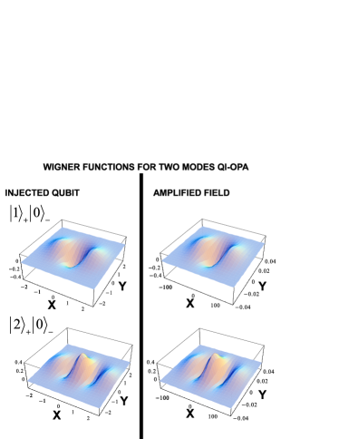
Figure 4: Wigner function of the injected states and the corresponding amplified states, for a non-degenerate amplifier with gain $g=4$. The axes scales on different graphs are different due to the high degree of squeezing introduced by the amplifier. $\left|1+,0-\right\rangle$ injection of a single photon $\vec{\pi}_{+}$ polarized. $\left|2+,0-\right\rangle$ injection of a two-photon state $\vec{\pi}_{+}$ polarized.

These Wigner functions can also be evaluated by employing the results obtained in the single mode amplifier case. In this context the characteristic function factorizes into two parts $\chi_{+}(\eta,t)\chi_{-}(\eta,t)$, that refer to polarizations $\vec{\pi}_{+}$ and $\vec{\pi}_{-}$ respectively, as a consequence of the independence of the two oscillators. Analogously, the Wigner function factorizes and when the state $\left|\psi_{in}\right\rangle=\left|1+,0-\right\rangle$ is injected, it reads:

$$W_{|1+,0-\rangle}(\tilde{\alpha},\tilde{\beta},t)=W_{+}(\tilde{\alpha})W_{-}(\tilde{\beta})=-\left(\frac{2}{\pi}\right)^{2}$$

$$\left[1-4\left|\bar{\alpha}\right|^{2}\right]\exp\left[-2\left|\bar{\alpha}\right|^{2}\right]\exp\left[-2\left|\bar{\beta}\right|^{2}\right]$$ (44)

where $\bar{\alpha}(t)=\tilde{\alpha}\cosh(g)-\tilde{\alpha}^{\ast}\sinh(g)$ and $\bar{\beta}(t)=\tilde{\beta}\cosh(g)-\tilde{\beta}^{\ast}\sinh(g)$. The variables $\left(\tilde{\alpha},\tilde{\beta}\right)$ are related to $\left(\alpha,\beta\right)$ through a simple rotation into the quadri-dimensional phase space:

$$\cosh\left(g\right)\alpha-\sinh\left(g\right)\beta^{\ast} = \cosh\left(g\right)\tilde{\alpha}-\sinh\left(g\right)\tilde{\alpha}^{\ast}$$ (45)

$$\cosh\left(g\right)\beta-\sinh\left(g\right)\alpha^{\ast} = \cosh\left(g\right)\tilde{\beta}-\sinh\left(g\right)\tilde{\beta}^{\ast}$$ (46)

We note that these rotations take the form of the Bogolioubov transformations which express the time evolution of the field operators in the collinear Optical Parametric Amplifier.

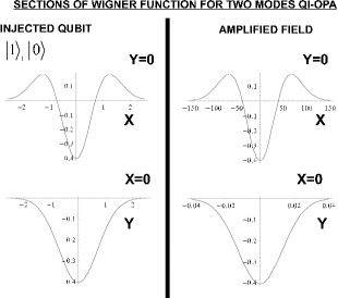
Figure 5: Sections of the Wigner function for the injection of the single photon state and for the corresponding amplified state obtained with a non-collinear amplifier with a gain value $g=4$.

III.3 Measurement of the quadratures with a double homodyne

Quadratures measurement can be obtained by homodyne technique Wall95 largely adopted in the context of quantum optics. Quantum fields showing quadratures entanglement have been realized Ou92 ; Zhan00 ; Silb01 ; Bowe03 ; Giac92 ; Scho02 and adopted in several quantum information protocols. We now discuss the realization of a double homodyne experiment in order to investigate the Wigner distributions in the QIOPA case. We define the quadrature operators in a general form, introducing the phase dependence from the variable $\theta$:

$$\hat{X}_{\theta}=\frac{\hat{a}e^{-i\theta}+\hat{a}^{\dagger}e^{i\theta}}{2};\hat{Y}_{\theta}=\frac{-i\hat{a}e^{-i\theta}+i\hat{a}^{\dagger}e^{i\theta}}{2}$$ (47)

Let us briefly review the scheme of an homodyne experiment. The impinging field under investigation $\hat{E}_{1}(\mathbf{r},t)$ is combined into a beam splitter with a local oscillator $\hat{E}_{L.O}(\mathbf{r},t)$, usually prepared in a coherent state $|\beta\rangle$ with $\beta=|\beta|e^{\imath\theta}$. When $\beta$ is larger than the amplitude of the field $\hat{E}_{1}$, the difference between the photon-counts of the two output modes of the beam-splitter is proportional to:

$$\langle\hat{c}^{\dagger}\hat{c}\rangle-\langle\hat{d}^{\dagger}\hat{d}\rangle\approx\sqrt{2\tau\left(1-\tau\right)}\langle\hat{Y}_{\theta}\rangle$$ (48)

where $\tau$ is the BS transmittivity. By varying the local oscillator phase by $\pi/2$ it is possible to select the measured quadrature.

In the context of the QI-OPA we need to generalize the homodyne measurement for the two polarization modes. A BS is inserted in the experimental scheme, following two different solutions. In the first case (Fig.6-(a)) at the exit of the QI-OPA a couple of waveplates $\lambda/4+\lambda/2$ and a PBS divide the two orthogonal polarizations which are combined with two equally polarized local oscillators.

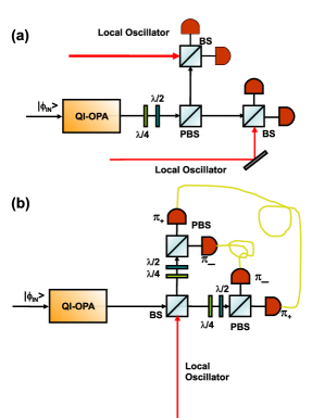
Figure 6: Two equivalent schemes for the double homodyne measurements. In both schemes, the choice of the basis for the analysis depends from the waveplates $\lambda/4+\lambda/2$ settings. (a) A PBS divides the two polarization components, each component is combined with a coherent radiation (with same polarization) on a BS. At the output of the PBS the field is revealed by two photodiodes. The signals are analyzed following the theory of the homodyne technique. (b) A BS combines the field with a local oscillator. The two output field impinge on a PBS which divides the two polarization components. The choice of the analysis basis depends on the waveplates setting $\lambda/4+\lambda/2$. Signals relative to the different polarization components are detected through two photodiodes and the results are pair-correlated according to homodyne theory.

In the second case (Fig.6-(b)) the field at the exit of the QI-OPA is combined with a local oscillator onto a BS; the two output modes are analyzed in polarization through a couple of waveplates $\lambda/4+\lambda/2$ (same setting on both modes) and a PBS and finally detected by a pair of photodiodes. The local oscillator polarization must be intermediate with respect to the analysis basis, for example if the analysis basis is the linear $\pm 45^{\circ}$ rotated one, the polarization of the local oscillator can be horizontal or vertical. The intensity measurements on both arms must be correlated, coupling equal polarizations in order to obtain the result of (48). The results obtained in the two configurations are equal, and the two schemes are completely equivalent for the characterization of QI-OPA amplified states.

III.4 Optical parametric amplification of N$>1$ Fock states

Let us now consider the two-photon input state $\left|\psi_{in}\right\rangle=\left|2+,0-\right\rangle$ the characteristic function reads:

$$\chi_{2,0}(\eta,\xi,t)=\exp[-\frac{1}{4}(\left|\eta(t)\right|^{2}+\left|\xi(t)\right|^{2})]\left(1-\left|\eta(t)\right|^{2}+\frac{\left|\eta(t)\right|^{4}}{8}\right)$$ (49)

and the Wigner function becomes:

$$W_{|2+,0-\rangle}(\alpha,\beta,t)=\left(\frac{2}{\pi}\right)^{2}e^{-\left|\Delta\right|^{2}}$$ (50)

$$\left(1-2\left|\Delta_{A}+\Delta_{B}\right|^{2}+\frac{1}{2}\left|\Delta_{A}+\Delta_{B}\right|^{4}\right)$$

A three dimensional plot of this function is obtained (see Fig. 4).

When both polarization modes are one photon injected $\left|\psi_{in}\right\rangle=\left|1+,1-\right\rangle$, the characteristic function reads:

$$\chi_{1,1}(\eta,\xi,t)=\left(1-\frac{\left|\eta(t)\right|^{2}}{2}\right)\left(1-\frac{\left|\xi(t)\right|^{2}}{2}\right)e^{-\frac{1}{4}(\left|\eta(t)\right|^{2}+\left|\xi(t)\right|^{2})}$$ (51)

and Wigner function is:

$$W_{|1+,1-\rangle}(\alpha,\beta,t) = \left(\frac{2}{\pi}\right)^{2}\left[1-2\left|\Delta\right|^{2}+\left|\Delta_{A}+\Delta_{B}\right|^{2}\times\right.$$ (52)

$$\times \left.\left(1-\left|\Delta_{A}+\Delta_{B}\right|^{2}\right)\right]e^{-\left|\Delta\right|^{2}}$$

As in the single mode case, we can generalize the results obtained for a generic Fock-state as input $|\psi_{in}\rangle=|N+,M-\rangle$. The Wigner functions of the amplified field with these generalized seeds read:

$$W_{|N+,M-\rangle}(\alpha,\beta,t) =\left(\frac{2}{\pi}\right)^{2}(-1)^{M+N}L_{N}\left(|\Delta_{A}+\Delta_{B}|^{2}\right)$$ (53)

$$L_{M}\left(|\Delta_{B}-\Delta_{A}|^{2}\right)e^{-2|\Delta|^{2}}$$

The Wigner function approach given in this Section to the QI-OPA device allows to stress the quantum properties of the amplified field. The negativity of the Wigner function can be deduced by the explicit general expression of Eq.(53). Indeed, in analogy with the un-amplified Fock-states $|N+,M-\rangle$ Schl01 , the Wigner function $W_{|N+,M-\rangle}(\alpha,\beta,t)$ is the product of two Laguerre polynomials Abra65 $L_{N}$ and $L_{M}$, which are negative in several region. Furthermore, the amplified states possess a high degree of squeezing in the field $\left\{\overline{\alpha},\overline{\beta}\right\}$ quadratures, at variance with the injected states.

IV Fock-Space analysis of macroscopic quantum superpositions over a lossy channel

In the present Section we analyze how the peculiar quantum interference properties of the amplified single-photon states are smoothed and cancelled when a decoherence process, i.e. a ”system-enviroment” interaction, is affecting their time evolution. More specifically, in the specific case of optical fields, the main decoherence process can be identified with the presence of lossy elements, as for example photo-detectors. Such process is mathematically described by an artificial beam-splitter (BS) scattering model, since this optical element expresses the coupling between the transmission channel and a different spatial mode. The same analysis is carried out also on a different class of MQS based on coherent $|\alpha\rangle$ states, to emphasize analogies and differences.

IV.1 The lossy channel model

As said, losses are analyzed through the effect of a generic linear beam-splitter (BS) with transmittivity $T$ and reflectivity $R=1-T$, acting on a generic quantum state associated with a single mode beam: Fig.7 Loud00 ; Durk04 ; Durk04a ; Leon93 . The action of the lossy channel on a generic density matrix $\hat{\rho}$ is obtained by the application of the BS unitary transformation and by the evaluation of the partial trace on the BS reflected mode (R-trace). The linear map describing the interaction is expressed by the following expansion Durk04 ; Durk04a :

$$\mathcal{L}[\hat{\rho}]=\sum_{p}\hat{M}_{p}\,\hat{\rho}\,\hat{M}_{p}^{{\dagger}}$$ (54)

where the $\hat{M}_{p}$ operators are:

$$\hat{M}_{p}=R^{p/2}T^{(\hat{a}^{{\dagger}}\hat{a})/2}\frac{\hat{a}^{p}}{\sqrt{p!}}$$ (55)

To evaluate the average values of operators, the lossy channel can be expressed in the Heisenberg picture, exploiting the BS unitary transformations and performing the average on the initial state $\hat{\rho}$.

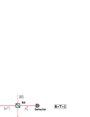
Figure 7: Schematization of the decoherence model by a linear beam-splitter of transmittivity T.

IV.2 De-coherence on the quantum superposition of coherent $|\alpha\rangle$ states

In this Section we investigate the evolution over a lossy channel of the quantum superpositions of coherent states (CSS) Schl91 :

$$|\Psi_{\pm}^{\varphi}\rangle{}=\mathcal{N}_{\pm}^{\varphi}\frac{1}{\sqrt{2}}\left(|\alpha e^{\imath\varphi}\rangle{}\pm|\alpha e^{-\imath\varphi}\rangle\right)$$ (56)

with $\alpha$ real and $\mathcal{N}_{\varphi}^{\pm}=\left(1\pm e^{-2|\alpha|^{2}\sin^{2}\varphi}\cos\left[|\alpha|^{2}\sin 2\varphi\right]\right)^{-\frac{1}{2}}$ is an appropriate normalization factor. The two states with opposite relative phases $|\Psi_{+}^{\varphi}\rangle{}$ and $|\Psi_{-}^{\varphi}\rangle{}$ are orthogonal when $|\alpha|^{2}\sin^{2}\varphi>1$ (Fig.8). In such case the two components $|\alpha e^{\imath\varphi}\rangle{}$ and $|\alpha e^{-\imath\varphi}\rangle$ are distinguishable. This class of Macroscopic Quantum Superposition presents several peculiar properties, such as squeezing and sub-poissonian statistics, which can not be explained by the characteristics of the coherent $|\alpha\rangle$ states.

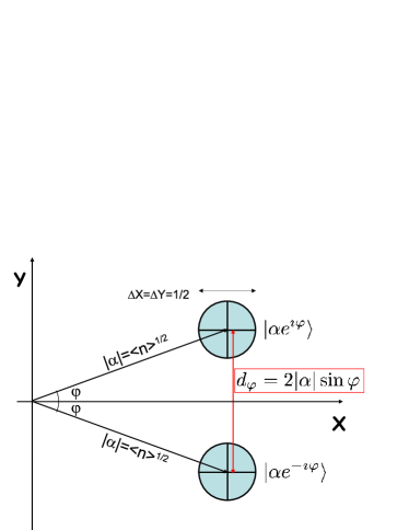
Figure 8: Schematic representation in the bidimensional phase-space $\left\{X,Y\right\}$ of the coherent states $|\alpha e^{\imath\varphi}\rangle$ which are the components of the MQS treated in this section. The circles represent the two-dimensional projection of the Gaussian functions which represent the Wigner function of these states. The distance between the center of the two Gaussian is $d_{\varphi}^{2}=4|\alpha|^{2}\sin^{2}\varphi$.

We now proceed with the analysis of the density matrix after the propagation over the lossy channel. In the following we assume $|\alpha|^{2}\sin^{2}\varphi>1$, hence $\mathcal{N}_{\varphi}^{\pm}\sim 1$. The density matrix of the quantum state after the beam-splitter transformation is:

$$\hat{\rho^{\prime}}^{\pm\,\varphi} =\frac{1}{2}\left(|\beta e^{\imath\varphi}\rangle_{C}\,{}_{C}\langle\beta e^{\imath\varphi}|\otimes|\imath\gamma e^{\imath\varphi}\rangle_{D}\,{}_{D}\langle\imath\gamma e^{\imath\varphi}|+\right.$$ (57)

$$+\left.|\beta e^{-\imath\varphi}\rangle_{C}\,{}_{C}\langle\beta e^{-\imath\varphi}|\otimes|\imath\gamma e^{-\imath\varphi}\rangle_{D}\,{}_{D}\langle\imath\gamma e^{-\imath\varphi}|\right.+$$

$$\pm\left.|\beta e^{\imath\varphi}\rangle_{C}\,{}_{C}\langle\beta e^{-\imath\varphi}|\otimes|\imath\gamma e^{\imath\varphi}\rangle_{D}\,{}_{D}\langle\imath\gamma e^{-\imath\varphi}|+\right.$$

$$\pm\left.|\beta e^{-\imath\varphi}\rangle_{C}\,{}_{C}\langle\beta e^{\imath\varphi}|\otimes|\imath\gamma e^{-\imath\varphi}\rangle_{D}\,{}_{D}\langle\imath\gamma e^{\imath\varphi}|\right)$$

with $\beta=\sqrt{T}\alpha$ and $\gamma=\sqrt{R}\alpha$. The output state over the transmitted field is obtained by tracing the density matrix $\hat{\rho^{\prime}}^{\pm\,\varphi}$ over the mode $\hat{d}$. The final expression for the density matrix after losses reads:

$$\hat{\rho}_{C}^{\pm} =\frac{1}{2}\left(|\beta e^{\imath\varphi}\rangle\,\langle\beta e^{\imath\varphi}|+|\beta e^{-\imath\varphi}\rangle\,\langle\beta e^{-\imath\varphi}|+\right.$$ (58)

$$\left.\pm e^{-2R|\alpha|^{2}\sin^{2}\varphi}e^{\imath R|\alpha|^{2}\sin 2\varphi}|\beta e^{\imath\varphi}\rangle\,\langle\beta e^{-\imath\varphi}|+\right.$$

$$\left.\pm e^{-2R|\alpha|^{2}\sin^{2}\varphi}e^{-\imath R|\alpha|^{2}\sin 2\varphi}|\beta e^{-\imath\varphi}\rangle\,\langle\beta e^{\imath\varphi}|\right)$$

Let us analyze first the case $\varphi=\frac{\pi}{2}$. The distribution in the Fock space exhibits only elements with an even number of photons for $|\Psi_{+}\rangle$ or an odd number of photons for $|\Psi_{-}\rangle$. This peculiar comb structure is indeed very fragile under the effect of losses since the R-trace operation must be carried out in the space of the non-orthogonal coherent-states. In fig.9 are reported the photon number distribution for different values of $R$ with an initial average number of photon equal to $\langle n\rangle=16$ and $\varphi=\frac{\pi}{2}$.

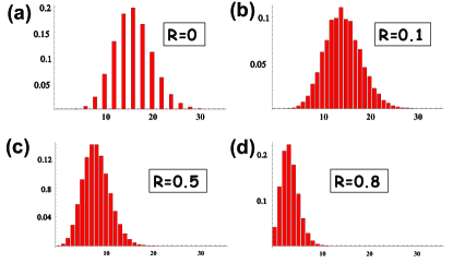
Figure 9: (a)-(d): Plot of the distribution of the number of photons in the $|\Psi_{+}^{\frac{\pi}{2}}\rangle$ state for $\alpha=4$, corresponding to an average number of photons $\langle n\rangle=16$, for reflectivities $R=0$ (fig.2-a), $R=0.1$ (fig.2-b), $R=0.5$ (fig.2-c) and $R=0.8$ (fig.2-d)

We observe that for a reflectivity $R=0.1$, corresponding to about $\sim 1.5$ photon lost in average, the distribution is similar to the Poisson distribution associated to the coherent states. Such graphical analysis points out how the ortoghonality between $|\Psi_{+}\rangle$ and $|\Psi_{-}\rangle$ quickly decrease as soon as $R$ differs from $0$, since the phase relation between the components $|\alpha\rangle$ and $|-\alpha\rangle$ becomes undefined.

IV.3 De-coherence in a lossy channel for equatorial amplified qubits

Analogously to the previous Section, in which the effect of losses where analyzed for the MQS of coherent state, we begin our treatment of QIOPA amplified states with the evaluation of the density matrix after the propagation over a lossy channel.

Before the lossy process, the density matrix of the state $\hat{\rho}^{\varphi}=|\Phi^{\varphi}\rangle\,\langle\Phi^{\varphi}|$ has the form:

$$\hat{\rho}^{\varphi}=\sum_{i,j,k,q=0}^{\infty}\gamma_{ij}\gamma^{\ast}_{kq}|(2i+1)\varphi,(2j)\varphi_{\bot}\rangle\,\langle(2k+1)\varphi,(2q)\varphi_{\bot}|$$ (59)

We note from this expression that only elements with an odd number of photons in the $\vec{\pi}_{\varphi}$ and an even number in the $\vec{\pi}_{\varphi_{\bot}}$ polarization are present. Furthermore, in Fig.10-(a) we note that the photon number distribution presents a strong unbalancement due to the quantum injection of the $\vec{\pi}_{\varphi}$ single photon. Indeed, the QIOPA seeded by a photon with equatorial polarization acts as a phase-covariant optimal cloning machine, and is stimulated to generate an output field containing more photons in the polarization of the injected seed. Let us now analyze the effects of the transmission in a lossy channel for the equatorial amplified qubits by plotting the photon number distributions. The output density matrix after the transmission over the lossy channel is the sum of four terms:

$$\hat{\rho}^{\varphi}_{T} =\sum_{i,j,k,q=0}^{\infty}\left(\hat{\rho}^{\varphi}_{T}\right)_{ijkq}|(2i+1)\varphi,(2j)\varphi_{\bot}\rangle\,\langle(2k+1)\varphi,(2q)\varphi_{\bot}|+\left(\hat{\rho}^{\varphi}_{T}\right)_{ijkq}|(2i)\varphi,(2j)\varphi_{\bot}\rangle\,\langle(2k)\varphi,(2q)\varphi_{\bot}|+$$ (60)

$$+\left(\hat{\rho}^{\varphi}_{T}\right)_{ijkq}|(2i+1)\varphi,(2j+1)\varphi_{\bot}\rangle\,\langle(2k+1)\varphi,(2q+1)\varphi_{\bot}|+\left(\hat{\rho}^{\varphi}_{T}\right)_{ijkq}|(2i)\varphi,(2j+1)\varphi_{\bot}\rangle\,\langle(2k)\varphi,(2q+1)\varphi_{\bot}|$$

The details on the calculation and on the expressions of the coefficients are reported in appendix A.

Let us now analyze this result. When the original state propagates through a lossy channel, the first effect at low values of $R$ is the cancellation of the peculiar comb structure (Fig.10-(a)) given by the presence in the density matrix (59) only of terms with a specific parity $|(2i+1)\varphi,(2j)\varphi_{\bot}\rangle\,\langle(2k+1)\varphi,(2q)\varphi_{\bot}|$, similarly to the coherent state MQS’s previously studied. However, at progressively higher values of $R$, the distributions in the Fock space remain unbalanced in the polarization of the injected photon (Fig.10-(a)). The resilience of this unbalancement allows to distinguish the orthogonal macro-qubits $\left\{|\Phi^{\varphi}\rangle,|\Phi^{\varphi_{\bot}}\rangle\right\}$ even after the propagation over the lossy channel, by exploiting this property with a suitable detection scheme, such as the OF device reported in DeMa08 . All these considerations will be discussed and quantified later in the paper in Section VII by analyzing the distinguishability of such states as a function of the lossy channel efficiency $T$.

IV.4 De-coherence in a lossy channel for amplified $\vec{\pi}_{H},\vec{\pi}_{V}$ qubits

For the sake of completeness, in this Section we shall analyze the evolution of $|\Phi^{H}\rangle$ and $|\Phi^{V}\rangle$ amplified states. As a first remark, we note that the collinear Optical Parametric Amplifier is not an optimal cloner for states with $\pi_{H}$ and $\pi_{V}$ polarization, and the output states do not possess the same peculiar properties obtained with an equatorial injected qubit. The density matrix of the $|\Phi^{H}\rangle$ amplified state is:

$$\hat{\rho}^{H} =|\Phi^{H}\rangle\,\langle\Phi^{H}|=\frac{1}{C^{4}}\sum_{n,m=0}^{\infty}\Gamma^{n+m}\sqrt{n+1}\sqrt{m+1}$$ (61)

$$|(n+1)H,nV\rangle\,\langle(m+1)H,mV|$$

In Fig.10-(b) we plotted the photon number distribution of this state (R=0). We note that the $\vec{\pi}_{H}$ amplified state does not possess the same unbalancement of the equatorial macro-qubits $|\Phi^{\varphi}\rangle$ analyzed in the previous section.

After the propagation over the lossy channel, the density matrix reads:

$$\hat{\rho}^{H}_{T}=\sum_{i=1}^{\infty}\sum_{j=0}^{i-1}\sum_{k=0}^{\infty}\left(\hat{\rho}^{H}_{T}\right)_{ijk}|iH,jV\rangle\,\langle kH,(k+j-i)V|+$$ (62)

$$+\sum_{i=0}^{\infty}\sum_{j=i}^{\infty}\sum_{k=0}^{\infty}\left(\hat{\rho}_{T}^{H}\right)_{ijk}|iH,jV\rangle\,\langle kH,(k+j-i)V|$$

where details on the calculation and on the coefficients are reported in appendix B. The effect of the propagation over the lossy channel is shown in Fig.10-(b). The original distribution for $R=0$ is pseudo-diagonal, corresponding to the presence only of terms $|(n+1)H,nV\rangle$. Here the difference of one photon between the two polarization is due to the injection of the seed. For values of $R$ different from 0, the distribution is no longer pseudo-diagonal and this characteristic becomes progressively smoothed. Furthermore, the absence of the unbalancement in the photon number distribution typical of the equatorial macro-qubits does not allow to exploit this feature to discriminate among the orthogonal states $\left\{|\Phi^{H}\rangle,|\Phi^{V}\rangle\right\}$. We then expect that these couple of states possess a lower resilience to losses than the equatorial $|\Phi^{\varphi}\rangle$ macro-states analyzed in the previous section.

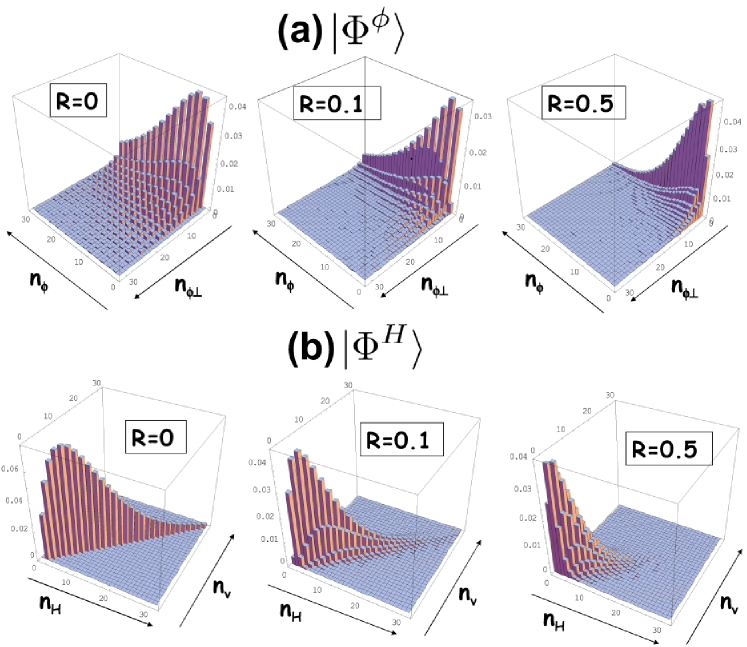
Figure 10: (a) Probability distribution in the Fock space $(n_{\phi},n_{\phi_{\bot}})$ for the amplified $|\Phi^{\phi}\rangle$ state of a generic equatorial qubit for different values of the transmittivity. (b) Probability distribution in the Fock space $(n_{H},n_{V})$ for the amplified $|\Phi^{H}\rangle$ state for different values of the transmittivity. All distributions refer to a gain value of $g=1.5$, corresponding to an average number of photons $\langle n\rangle\approx 19$.

V Wigner function representation of coherent states MQS in presence of de-coherence

For the sake of clarity, we briefly review previous results on the Wigner functions associated to coherent superposition states after the propagation over a lossy channel. We start from the general definition of the Wigner function for mixed states Wign32 :

$$W_{\hat{\rho}}(X,Y)=\frac{1}{\pi}\int_{-\infty}^{\infty}d\xi e^{2\imath Y\xi}\langle X-\xi|\hat{\rho}|X+\xi\rangle$$ (63)

Considering the density matrix of the CSS after losses (58) we obtain:

$$W_{\hat{\rho}_{C}^{\varphi\,\pm}}(X,Y) =\frac{\mathcal{N}^{\varphi\,2}_{\pm}}{2}\left(W_{|\beta e^{\imath\varphi}\rangle{}}(X,Y)+W_{|\beta e^{-\imath\varphi}\rangle{}}(X,Y)+\right.$$ (64)

$$\left.\pm W^{int}_{\hat{\rho}_{C}^{\varphi\,\pm}}(X,Y)\right)$$

In the last expression, the first two components are analogous to the diagonal ones of the unperturbed case Schl91 , and can be written as :

$$W_{|\beta e^{\pm\imath\varphi}\rangle{}}(X,Y)=\frac{1}{\pi}e^{-\left(X-\sqrt{T}\overline{x}_{\varphi}\right)^{2}}e^{-\left(Y\mp\sqrt{T}\overline{Y}_{\varphi}\right)^{2}}$$ (65)

where $\overline{X}_{\varphi}^{2}=2|\alpha|^{2}\cos^{2}\varphi$ and $\overline{Y}_{\varphi}^{2}=2|\alpha|^{2}\sin^{2}\varphi$. Hence losses reduce the average value of the quadratures $\hat{X}$ and $\hat{Y}$.

The interference contribution reads:

$$W^{int}_{\hat{\rho}_{C}^{\varphi\,\pm}} (X,Y)=\frac{2}{\pi}e^{-Y^{2}}e^{-\left(X-\sqrt{T}\overline{X}_{\varphi}\right)^{2}}e^{-R\overline{Y}_{\varphi}^{2}}\times$$ (66)

$$\times\cos\left[2\sqrt{2}\alpha\sqrt{T}\sin\varphi\left(X-\frac{\alpha(2T-1)}{\sqrt{2T}}\cos\varphi\right)\right]$$

which is strongly reduced in amplitude by a factor proportional to $e^{-R\overline{Y}_{\varphi}^{2}}$.

In Fig.11 are plotted the Wigner functions associated to different values of $R$, for the same initial conditions $\varphi=\frac{\pi}{2}$ and $\alpha=6$.

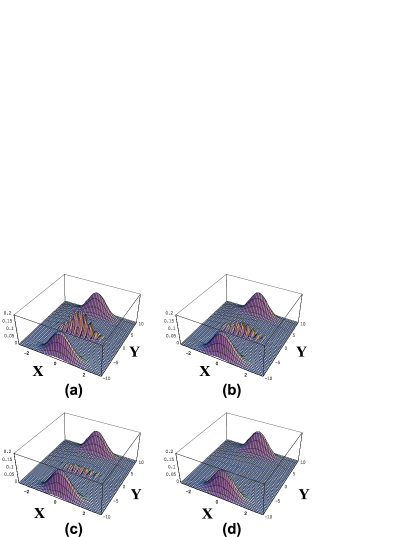
Figure 11: Plots of the Wigner function for $\alpha=6$ and $\varphi=\frac{\pi}{2}$ for different values of the riflectivity (a) $R=0$, (b) $R=0.01$, (c) $R=0.02$ and (d) $R=0.1$.

As expected, by increasing the degree of losses the central peak is progressively attenuated up to a complete deletion of the quantum features associated to the negativity of the Wigner functions. We observe that the damping factor $e^{-2R|\alpha|^{2}\sin^{2}\varphi}$ of the coherence terms derives from the exponential decrease of the non-diagonal terms of the density matrix (58).

More specifically, we now focus on the $\varphi=\frac{\pi}{2}$ case, i.e. the $|\alpha\rangle\pm|-\alpha\rangle$ state. In Fig. 12 we report the plots of the $Y=0$ section of the Wigner function for different values of the reflectivity $R$, which corresponds to the interference pattern.

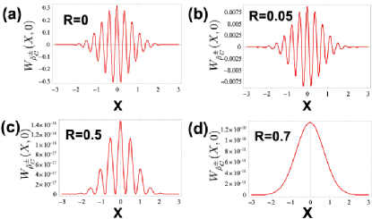
Figure 12: $Y=0$ sections of the Wigner function for the quantum superposition of coherent states, for $\alpha=6$ and $\varphi=\frac{\pi}{2}$ and different values of $R$. (a) $R=0$: Unperturbed interference pattern. (b) $R=0.05$: Exponentially damped interference pattern. (c) $R=0.5$: Transition to a completely positive Wigner function, as the interference pattern is shifted towards positive values. (d) $R=0.7$: The interference pattern in the central region is deleted by decoherence.

At low R, the amplitude of the oscillation is exponentially damped. This exponential factor $e^{-2R|\alpha|^{2}\sin^{2}\varphi}$ is responsible for the fast decrease in the negativity of the Wigner function, but the alternance of positive and negative regions is maintained. However, when $R$ approaches the $0.5$ value, the interference pattern is progressively shifted towards positive values in all the X-axis range, and at $R=0.5$ it ceases to be non-positive. This evolution depends on the presence of the $W_{|\beta e^{\pm\imath\varphi}\rangle{}}(X,Y)$ diagonal terms, which are not exponentially damped in amplitude and for $R\sim 0.5$ become comparable to the interference term. This transition is graphically shown in Fig.13, where the negativity is plotted as a function of $R$. This quantity has been evaluated by calculating the value of the Wigner function in the first minimum of the cosine term of $W^{int}_{\hat{\rho}_{C}^{\varphi\,\pm}}(X,Y)$. We note the transition from negative to positive at $R=0.5$, where for higher values this point ceases to be the minimum of the complete Wigner function in the $\left\{X,Y\right\}$ plane.

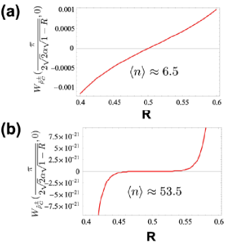
Figure 13: Transition from non-positive to completely positive Wigner function as a function of the reflectivity $R$, for a number of average photons of $\langle n\rangle\approx 6.5$ (a) and $\langle n\rangle\approx 53.5$ (b). The negativity has been evaluated as described in the text. We note that, while the interval of $R$ in which the Wigner function is non positive is independent of the number of photons, the amount of negativity decreases exponentially with $\langle n\rangle$ due to the exponential factor $e^{-2R|\alpha|^{2}\sin^{2}\varphi}$ in the interference term $W^{int}_{\hat{\rho}_{C}^{\varphi\,\pm}}(X,Y)$.

This property can be derived explicitly by the complete form of the Wigner function. For $\varphi=\frac{\pi}{2}$, $Y_{0}=0$ and $X_{0}=\frac{\pi}{2\sqrt{2}\sqrt{1-R}\alpha}$, corresponding to the minimum of the cosine $\cos\left[2\sqrt{2}\alpha\sqrt{T}\sin\varphi\left(X-\frac{\alpha(2T-1)}{\sqrt{2T}}\cos\varphi\right)\right]$, we get:

$$W_{\hat{\rho}_{C}^{\frac{\pi}{2}\,+}}(X_{0},0) =\frac{\mathcal{N}^{\frac{\pi}{2}}_{+}}{\pi}e^{-2(1-R)|\alpha|^{2}}\left(e^{-2|\alpha|^{2}(1-R)}-e^{-2|\alpha|^{2}R}\right)=$$ (67)

$$=\left\{\begin{array}[]{lrl}<0&\mathrm{if}&R<\frac{1}{2}\\ >0&\mathrm{if}&R>\frac{1}{2}\end{array}\right.$$

thus obtaining the desired result.

As a general statement, it is well known that the negativity of the ”quasi-probability” Wigner function of a state $\rho$ is a sufficient, albeit non necessary, condition for the ”quantumness” of $\rho$Schl01 .

VI Wigner function representation of the phase-covariant quantum cloning process in presence of de-coherence

Combining the approach of Section III and the lossy channel method introduced in Section IV, we derive the analytical expressions for the Wigner function of the QI-OPA amplified states in presence of losses. The calculation will be performed in the Heisenberg picture, starting from the evaluation of the characteristic function of the BS-transmitted field. This analysis will be performed for both the single-mode degenerate amplifier, i.e. a single-mode squeezing Hamiltonian, and for the two-mode optical parametric amplifier, in which the polarization degree of freedom plays an important role as stressed in the Fock-space analysis previuosly performed. Finally, we shall focus our attention on the negativity of the Wigner function, evidence of the non-classical properties of this class of states.

VI.1 Single-mode degenerate amplifier

Let us first analyze the case of a single mode-degenerate amplifier. We begin our analysis by evaluating the characteristic function in presence of a lossy channel. The operators describing the output field can be written in the Heisenberg picture in the form:

$$\hat{c}^{{\dagger}}(t)=\sqrt{T}\hat{a}^{{\dagger}}(t)+\imath\sqrt{R}\hat{b}^{{\dagger}}$$ (68)

where $\hat{a}^{{\dagger}}(t)=\hat{a}^{{\dagger}}\cosh g+\hat{a}\sinh g$ is the time evolution of the field operator in the amplifier, and $R=1-T$. Hence, the characteristic function for a generic input state $|N\rangle_{A}|0\rangle_{B}$ can be calculated as:

$$\chi_{N}(\eta,R,t)=\langle N,0|e^{\eta\hat{c}^{{\dagger}}(t)-\eta^{\ast}\hat{c}(t)}|N,0\rangle$$ (69)

Inserting the explicit expression (68) for the output field operators, we obtain the expression:

$$\begin{split}\chi_{N}(\eta,R,t)&=e^{-\frac{1}{2}T|\eta(t)|^{2}}\,e^{-\frac{1}{2}R|\eta|^{2}}\times\\ &\times\left[\sum_{n=0}^{N}\begin{pmatrix}N\\ n\end{pmatrix}\frac{(-1)^{n}}{n!}\left(T|\eta(t)|^{2}\right)^{n}\right]\end{split}$$ (70)

In this expression, the transformation $\left(\eta,\eta^{\ast}\right)\rightarrow\left(\eta(t),\eta^{\ast}(t)\right)$ has the form $\eta(t)=\eta C-\eta^{\ast}S$, equivalent to the ideal case previously analyzed. The Wigner function of the output field is then obtained from its definition (20) as the two-dimensional Fourier transform of the characteristic function. Inserting the explicit expression of $\chi_{N}(\eta,R,t)$, and by changing the variables with the transformation $\eta\rightarrow\eta(t)$ with unitary Jacobian we obtain:

$$\begin{split}W_{|N\rangle}(\alpha,R,t)&=\frac{1}{\pi^{2}}\sum_{n=0}^{N}c_{n}^{N}\int d^{2}\eta(t)\,|\eta(t)|^{2n}\,e^{-\varepsilon|\eta(t)|^{2}}\\ &\times\exp\left[-\kappa\left(\eta^{2}(t)+\eta^{\ast\,2}(t)\right)\right]\\ &\times\exp\left[-\overline{\alpha}^{\ast}\,\eta(t)+\overline{\alpha}\,\eta^{\ast}(t)\right]\end{split}$$ (71)

where:

$$c_{n}^{N} = \begin{pmatrix}N\\ n\end{pmatrix}\frac{(-1)^{n}}{n!}T^{n}$$ (72)

$$\varepsilon = \frac{1}{2}\left(1+2RS^{2}\right)$$ (73)

$$\kappa = \frac{1}{2}RCS$$ (74)

$$\overline{\alpha} = \alpha C-\alpha^{\ast}S$$ (75)

In order to evaluate the integral in the previous expression, we recall the following identity Bisw07 ; Puri01 :

$$\begin{split}&\frac{1}{\pi}\int d^{2}\alpha\,e^{-\tau|\alpha|^{2}}\exp\left[-\mu\alpha^{2}-\nu\alpha^{\ast\,2}-z^{\ast}\alpha+z\alpha^{\ast}\right]=\\ &=\frac{1}{\sqrt{\tau^{2}-4\mu\nu}}\exp\left[-\frac{\mu z^{2}+\nu z^{\ast\,2}+\tau|z|^{2}}{\tau^{2}-4\mu\nu}\right]\end{split}$$ (76)

From the latter equation, we can derive the following useful identities:

$$\begin{split}I_{n}\left(\mu,\nu,\tau,z\right)&=\frac{1}{\pi}\int d^{2}\alpha\,|\alpha|^{2n}e^{-\tau|\alpha|^{2}}\exp\left[-\mu\alpha^{2}-\nu\alpha^{\ast\,2}-z^{\ast}\alpha+z\alpha^{\ast}\right]=\\ &=\frac{1}{\pi}(-1)^{n}\frac{\partial^{2n}}{\partial z^{n}\partial z^{\ast\,n}}\int d^{2}\alpha e^{-\tau|\alpha|^{2}}\exp\left[-\mu\alpha^{2}-\nu\alpha^{\ast\,2}-z^{\ast}\alpha+z\alpha^{\ast}\right]=\\ &=(-1)^{n}\frac{\partial^{2n}}{\partial z^{n}\partial z^{\ast\,n}}\left\{\frac{1}{\sqrt{\tau^{2}-4\mu\nu}}\exp\left[-\frac{\mu z^{2}+\nu z^{\ast\,2}+\tau|z|^{2}}{\tau^{2}-4\mu\nu}\right]\right\}\end{split}$$ (77)

These expressions can then be used to evaluate the Fourier transform of the characteristic function (70), leading to the Wigner function:

$$W_{|N\rangle}(\alpha,R,t)=\frac{1}{\pi}\sum_{n=0}^{N}c_{n}^{N}I_{n}\left(\kappa,\kappa,\varepsilon,\overline{\alpha}\right)$$ (78)

As a first case, we analyze the evolution of the Wigner function of a squeezed vacuum state, corresponding to the value $N=0$ in the previous expression. Analogously to the unperturbed case, the quadrature variables for the single-mode OPA are defined by $\alpha=X+\imath Y$. The Wigner function for the squeezed vacuum then reads:

$$\begin{split}&W_{|0\rangle}(X,Y,R,t)=\frac{2}{\pi}\frac{1}{\sqrt{1+4(1-R)RS^{2}}}\\ &\times\exp\left[-2\frac{\left(X^{2}e^{-2g}+Y^{2}e^{2g}\right)+2RS\left(X^{2}e^{-g}+Y^{2}e^{g}\right)}{1+4(1-R)RS^{2}}\right]\end{split}$$ (79)

From this quantity, we can explicitly calculate how the degree of squeezing changes with an increasing value of the parameter R. We obtain for the fluctuations of the two field quadrature operators $\left\{\hat{X},\hat{Y}\right\}$ (Fig.14-(a)):

$$\Delta X = \frac{1}{2}\sqrt{Te^{2g}+(1-T)}$$ (80)

$$\Delta Y = \frac{1}{2}\sqrt{Te^{-2g}+(1-T)}$$ (81)

This two operators do not satisfy anymore the minimum uncertainty relation, as in the unperturbed case, after the propagation over the lossy channel: Fig.14-(b). This is due to the additional poissonian noise belonging to the photon loss process.

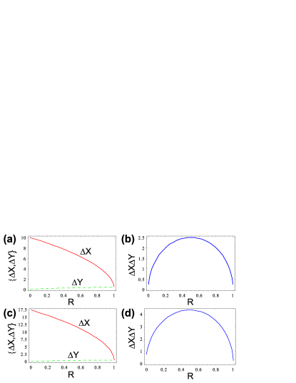
Figure 14: (a)-(b) Uncertainty relations for the quadrature operators in the spontaneous emission case for a single mode OPA. Left figure: Fluctuation on the $X$ quadrature (red straight line) and on the $Y$ quadrature (green dashedline) as a function of the parameter $R$ of the lossy channel. Right figure: Uncertainty relation $\Delta X\Delta Y$ as a function of the parameter $R$. (c)-(d) Uncertainty relations for the quadrature operators in the single-photon amplified case for a single mode OPA. Left figure: Fluctuation on the $X$ quadrature (red straight line) and on the $Y$ quadrature (green dashed line) as a function of the parameter $R$ of the lossy channel. Right figure: Uncertainty relation $\Delta X\Delta Y$ as a function of the parameter $R$. All figures refer to a gain value of $g=3$.

A similar behaviour is obtained for the single-photon squeezed state. The Wigner function for $N=1$ reads:

$$\begin{split}&W_{|1\rangle}(X,Y,R,t)=\frac{2}{\pi}\frac{1}{\sqrt{1+4(1-R)RS^{2}}}\,P_{|1\rangle}(X,Y,R,t)\\ &\times\exp\left[-2\frac{\left(X^{2}e^{-2g}+Y^{2}e^{2g}\right)+2RS\left(X^{2}e^{-g}+Y^{2}e^{g}\right)}{1+4(1-R)RS^{2}}\right]\end{split}$$ (82)

where:

$$\begin{split}&P_{|1\rangle}(X,Y,R,t)=1-\frac{4(1-R)}{1+4(1-R)RS^{2}}\left[\frac{1}{2}\left(1+2RS^{2}\right)+\right.\\ &+\left(X^{2}e^{-2g}+Y^{2}e^{2g}\right)+2\left(1+2RS^{2}\right)\times\\ &\times\left.\frac{\left(X^{2}e^{-2g}+Y^{2}e^{2g}\right)+2RS\left(X^{2}e^{-g}+Y^{2}e^{g}\right)}{1+4(1-R)RS^{2}}\right]\end{split}$$ (83)

The region where the Wigner function is negative becomes smaller when the parameter $R$ of the lossy channel is increased. In Fig.15 we report the plots of $W_{|1\rangle}(X,Y,R,t)$ for different values of the reflectivity $R$. As a first effect, the negative region is deleted for a reflectivity $R=1/2$: Fig.15-(d). Then, the form of the distribution remain unchanged until the reflectivity becomes close to 1 and all the photons present in the states are lost: $R\langle n\rangle\simeq\langle n\rangle$. As a further analysis, let us consider the value at $X=0$ and $Y=0$, in which the Wigner function has the maximum negativity. We obtain that $W_{|1\rangle}(0,0,R,t)<0$ for $R\leq\frac{1}{2}$, showing that the negativity is maintained in that range of the lossy channel efficiency. This property can be analyzed by the two-dimensional contour plots of fig.16.

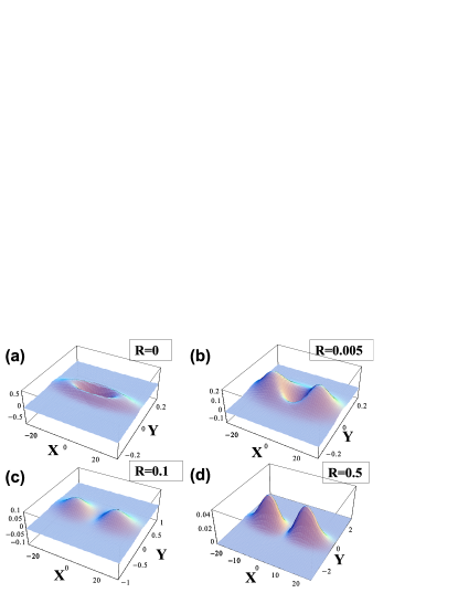
Figure 15: Wigner function of a single-photon amplified state in a single-mode degenerate OPA for $g=3$. (a) (R=0) Unperturbed case. (b) (R=0.005) For small reflectivity, the Wigner function remains negative in the central region. (c) (R=0.1) The Wigner function progressively evolve in a positive function in all the phase-space. (d) (R=0.5) Transition from a non-positive to a completely positive Wigner function.

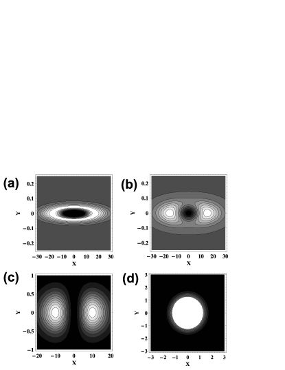
Figure 16: Contour plots of the Wigner function of a single-photon amplified state in a single-mode degenerate OPA for $g=3$. (a) (R=0) Unperturbed case. (b) (R=0.005) For small reflectivity, the Wigner distribution begin to evolve in a double-peaked function with a negative central region, analogously to the CSS case. (c) (R=0.5) Transition from the regime with a negative central region and a completely positive distribution (d) (R=1) Evolution of the Wigner function into a vacuum state when all photons are lost.

As a further analysis, starting from the Wigner function, we can evaluate the fluctuations in the quadrature operators after losses (Fig.14-(c):

$$\Delta X = \frac{1}{2}\sqrt{3Te^{2g}+(1-T)}$$ (84)

$$\Delta Y = \frac{1}{2}\sqrt{3Te^{-2g}+(1-T)}$$ (85)

As in the squeezed vacuum case, poissonian noise added by the lossy channel increases the fluctuations $\Delta X\Delta Y$ for any non-zero value of the losses parameter $R$: Fig.14-(d).

VI.2 Two-mode collinear amplifier

The previous calculation, performed in the case of a single-mode degenerate OPA, can be again used to analyze the collinear QI-OPA case. The characteristic function with a generic input two-mode state $|\Psi_{in}\rangle$ can be evaluated as:

$$\begin{split}\chi_{N,M}(\eta,\xi,R,t)&=\langle\Psi_{in}|e^{\eta\hat{c}^{{\dagger}}_{H}(t)-\eta^{\ast}\hat{c}_{H}(t)}\otimes\\ &\otimes e^{\xi\hat{c}^{{\dagger}}_{V}(t)-\xi^{\ast}\hat{c}_{V}(t)}|\Psi_{in}\rangle\end{split}$$ (86)

Analogously to the single-mode OPA case, the time evolution of the field operators, due to the amplification process and to the propagation in the lossy channel, takes the form:

$$\hat{c}^{{\dagger}}_{H}(t) = \sqrt{1-R}\,\hat{a}^{{\dagger}}_{H}(t)+\imath\sqrt{R}\,\hat{b}_{H}^{{\dagger}}$$ (87)

$$\hat{c}^{{\dagger}}_{V}(t) = \sqrt{1-R}\,\hat{a}^{{\dagger}}_{V}(t)+\imath\sqrt{R}\,\hat{b}_{V}^{{\dagger}}$$ (88)

where the expressions of the equation of motion for $\hat{a}_{H,V}^{{\dagger}}(t)$ are (4). We now proceed by writing the characteristic function in the $\left\{\vec{\pi}_{+},\vec{\pi}_{-}\right\}$ basis and by substituting the relations (87-88) for the time evolution in the Heisenberg picture of the field operators. The characteristic function then reads:

$$\begin{split}&\chi_{N,M}(\eta,\xi,R,t)=\langle\Psi_{in}|e^{\frac{\eta(t)\sqrt{1-R}}{\sqrt{2}}\hat{a}^{{\dagger}}_{+}-\frac{\eta^{\ast}(t)\sqrt{1-R}}{\sqrt{2}}\hat{a}_{+}}\\ &\otimes e^{\frac{\imath\sqrt{R}(\eta+\xi)}{\sqrt{2}}\hat{b}^{{\dagger}}_{+}-\frac{-\imath\sqrt{R}(\eta^{\ast}+\xi^{\ast})}{\sqrt{2}}\hat{b}_{+}}\otimes e^{\frac{\xi(t)\sqrt{1-R}}{\sqrt{2}}\hat{a}^{{\dagger}}_{-}-\frac{\xi^{\ast}(t)\sqrt{1-R}}{\sqrt{2}}\hat{a}_{-}}\\ &\otimes e^{\frac{\imath\sqrt{R}(\xi-\eta)}{\sqrt{2}}\hat{b}^{{\dagger}}_{-}-\frac{-\imath\sqrt{R}(\xi^{\ast}-\eta^{\ast})}{\sqrt{2}}\hat{b}_{-}}|\Psi_{in}\rangle\end{split}$$ (89)

The transformation between $\left(\eta,\eta^{\ast},\xi,\xi^{\ast}\right)\rightarrow\left(\eta(t),\eta^{\ast}(t),\xi(t),\xi^{\ast}(t)\right)$ is the same (34-35) of the unperturbed case. The evaluation of the average on an input injected state $|N+,M-\rangle$ in the QI-OPA and on the vacuum-injected port $b$ of the beam-splitter leads to the following result:

$$\begin{split}&\chi_{N,M}(\eta,\xi,R,t)=e^{-\frac{1}{4}R\left(|\eta+\xi|^{2}+|\xi-\eta|^{2}\right)}\\ &e^{-\frac{1}{4}(1-R)\left(|\eta(t)|^{2}+|\xi(t)|^{2}\right)}\left\{\sum_{n=0}^{N}\sum_{m=0}^{M}c_{n}^{N}c_{m}^{M}\right.\\ &\left.\left(\frac{|\eta(t)|^{2}}{2}\right)^{n}\left(\frac{|\xi(t)|^{2}}{2}\right)^{m}\right\}\end{split}$$ (90)

The Wigner function is then calculated as the 4-dimensional Fourier transform of the characteristic function. Analogously to the single-mode case, we proceed with the calculation by evaluating the Fourier integral that, after changing the integration variables with the transformation $\left(\eta,\eta^{\ast},\xi,\xi^{\ast}\right)\rightarrow\left(\eta(t),\eta^{\ast}(t),\xi(t),\xi^{\ast}(t)\right)$, can be written as:

$$\begin{split}W_{|N+,M-\rangle}(\alpha,\beta,R,t)&=\frac{1}{\pi^{4}}\int d^{2}\eta(t)\int d^{2}\xi(t)|J|\exp\left[-\frac{1}{2}\varepsilon\left(|\eta(t)|^{2}+|\xi(t)|^{2}\right)\right]\exp\left[-\frac{1}{2}\kappa\left(\eta^{2}(t)+\eta^{\ast\,2}(t)-\xi^{2}(t)-\xi^{\ast\,2}(t)\right)\right]\\ &\left(\sum_{n=0}^{N}c_{n}^{N}\frac{|\eta(t)|^{2n}}{2^{n}}\right)\left(\sum_{m=0}^{M}c_{m}^{M}\frac{|\xi(t)|^{2m}}{2^{m}}\right)\exp\left[\frac{1}{\sqrt{2}}\left(\eta^{\ast}(t)\overline{\alpha}-\eta(t)\overline{\alpha}^{\ast}\right)\right]\exp\left[\frac{1}{\sqrt{2}}\left(\xi^{\ast}(t)\overline{\beta}-\xi(t)\overline{\beta}^{\ast}\right)\right]\end{split}$$ (91)

where the parameters $\varepsilon,\kappa$ have been defined in (73-74), and the transformation between $\alpha\rightarrow\overline{\alpha}$ and $\beta\rightarrow\overline{\beta}$ is:

$$\overline{\alpha} = \frac{1}{\sqrt{2}}\left[(\alpha+\beta)C-(\alpha^{\ast}+\beta^{\ast})S\right]$$ (92)

$$\overline{\beta} = \frac{1}{\sqrt{2}}\left[(\beta-\alpha)C+(\beta^{\ast}-\alpha^{\ast})S\right]$$ (93)

The derived integral relations (77) lead to the final result:

$$\begin{split}W_{|N+,M-\rangle}(\alpha,\beta,R,t)&=\frac{1}{\pi^{2}}\left(\sum_{n=0}^{N}c_{n}^{N}I_{n}(\kappa,\kappa,\varepsilon,\overline{\alpha})\right)\\ &\times\left(\sum_{m=0}^{M}c_{m}^{M}I_{m}(-\kappa,-\kappa,\varepsilon,\overline{\beta})\right)\end{split}$$ (94)

Let us analyze the spontaneous emission case, when $N=M=0$. Adopting the same definition of the phase space used in the unperturbed case in Section III.2, we obtain:

$$\begin{split}W&{}_{|0+,0-\rangle}(X,Y,R,t)=\left(\frac{2}{\pi}\right)^{2}\frac{1}{1+4S^{2}R(1-R)}\\ &\times\exp\left[-\frac{\left(1+2RS^{2}+2RCS\right)X^{2}e^{-2g}}{1+4S^{2}R(1-R)}\right]\\ &\times\exp\left[-\frac{\left(1+2RS^{2}-2RCS\right)Y^{2}e^{2g}}{1+4S^{2}R(1-R)}\right]\end{split}$$ (95)

As in the single mode case, the degree of squeezing in the quadrature operators is progressively decreased by the poissonian noise introduced by the lossy channel.

Furthermore, let us analyze the case of the single photon amplified states, i.e. $N=1,M=0$ and $N=0,M=1$. The Wigner functions after losses for this quantum states are:

$$W_{|1+,0-\rangle}(X,Y,R,t) = W_{|0+,0-\rangle}\,P_{|1+,0-\rangle}(X,R,t)$$ (96)

$$W_{|0+,1-\rangle}(X,Y,R,t) = W_{|0+,0-\rangle}\,P_{|0+,1-\rangle}(Y,R,t)$$ (97)

where $P_{|1+,0-\rangle}(X,R,t)$ and $P_{|0+,1-\rangle}(Y,R,t)$ are the following $2^{nd}$ order polynomials:

$$\begin{split}P_{|1+,0-\rangle}&(X,R,t)=1+\frac{4(1-R)}{1+4S^{2}R(1-R)}\times\\ &\times\left[-\frac{1}{2}\left(1+X^{2}e^{-2g}\right)-RS^{2}+\left(1+2RS^{2}\right)\times\right.\\ &\times\left.\frac{1+2RS^{2}+2RCSX^{2}e^{-2g}}{1+4R(1-R)S^{2}}\right]\end{split}$$ (98)

$$\begin{split}P_{|0+,1-\rangle}&(Y,R,t)=1+\frac{4(1-R)}{1+4S^{2}R(1-R)}\times\\ &\times\left[-\frac{1}{2}\left(1+Y^{2}e^{2g}\right)-RS^{2}+\left(1+2RS^{2}\right)\times\right.\\ &\times\left.\frac{1+2RS^{2}-2RCSY^{2}e^{2g}}{1+4R(1-R)S^{2}}\right]\end{split}$$ (99)

In Fig.17 we report the Wigner function $W_{|1+,0-\rangle}(X,Y,R,t)$ for different values of the reflectivity $R$. The evolution of this distribution is similar to the single-mode OPA case analyzed previously.

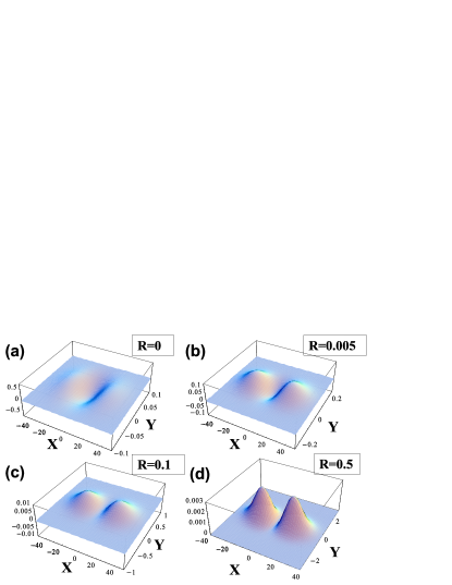
Figure 17: Wigner function of a single-photon $|1+\rangle$ amplified state in a two-mode degenerate OPA for $g=3$. (a) (R=0) Unperturbed case. (b) (R=0.005) For small reflectivity, the Wigner function remains negative in the central region. (c) (R=0.1) The Wigner function progressively evolve in a positive function in all the phase-space. (d) (R=0.5) Transition from a non-positive to a completely positive Wigner function.

VI.3 Resilience of quantum properties after decoherence

The Wigner functions calculated in the previous section allows to obtain a complete overview of the phase-space properties of the QI-OPA amplified states after the propagation over a lossy channel. In particular, we focus on the negativity of the W-representation in the specific case of a single-photon injected qubit. As said, the presence of a negative region in the phase-space domain is one possible parameter to recognize the non-classical properties of a generic quantum state.

Let us now consider the expression (98) for the polynomial $P_{|1+,0-\rangle}(X,R,t)$. In the lossless regime considered in Fig.4, the Wigner function takes its minimum value in the origin of the phase-space (X=0,Y=0). In presence of losses, the Wigner function remains negative in the origin for $R<\frac{1}{2}$. This behaviour is shown in the plots of the $Y=0$ sections of $W_{|1+,0-\rangle}(X,Y,R,t)$ reported in Fig.18, where for the value of $R=\frac{1}{2}$ ceases to be negative. This is also shown in Fig.19, that reports the value of $W_{|1+,0-\rangle}(0,0,R,t)$ as a function of the reflectivity $R$ of the beam-splitter that models the lossy channel. Finally, this behaviour, as for the quantum superposition of coherent states in the previous Section, can be analytically obtained by calculating $P_{|1+,0-\rangle}(X,R,t)$ in $X=0$. We obtain:

$$P_{|1+,0-\rangle}(X,R,t)=\frac{2R-1}{1+4R(1-R)S^{2}}\left\{\begin{array}[]{lrl}<0&\mathrm{if}&R<\frac{1}{2}\\ >0&\mathrm{if}&R>\frac{1}{2}\end{array}\right.$$ (100)

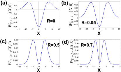
Figure 18: $Y=0$ section of the Wigner function for QIOPA single photon amplified states for $\langle n\rangle\approx 36$. (a) $R=0$: Unperturbed Wigner function, negative in the origin. (b) $R=0.05$: The negativity in the origin progressively decreases due to the coupling with the enviroment. (c) $R=0.5$: Transition from a non-positive to a completely positive Wigner function. (d) $R=0.7$: The Wigner function is positive in all the $\left\{X,Y\right\}$ plane.

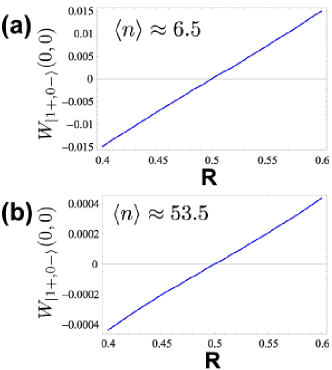
Figure 19: Transition from a non-positive distribution to a completely positive Wigner function for QI-OPA single-photon amplified states in presence of decoherence, as a function of the beam-splitter reflectivity $R$. Average photon number of (a) $\langle n\rangle\approx 6.5$ and (b) $\langle n\rangle\approx 53.5$. The negativity is evaluated as the value of the Wigner function in the origin.

This analysis explicitly shows the persistence of quantum properties in the QI-OPA single-photon amplified state even in presence of losses. However, the negativity of the Wigner function is not the only parameter that reveals the quantum behaviour in a given system. Hence, more detailed analysis have to be performed including different approaches in order to investigate the $R>\frac{1}{2}$ regime.

We conclude our analysis by comparing the behaviour of the two different macroscopic quantum superpositions analyzed in this paper. In Fig. 20 we compare the decrease of the Wigner function negativity for the QI-OPA single-photon amplified states and for the superposition of coherent states, for two different values of the average number of photons. We observe that the QI-OPA solution possesses a higher resilience to losses, i.e. a slower decrease of the negative part, with respect to the $|\alpha\rangle\pm|-\alpha\rangle$ states. However, the Wigner function for both quantum superposition ceases to be negative at $R=\frac{1}{2}$.

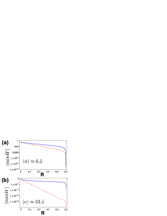
Figure 20: Absolute value of the negativity, evaluated as the minimum of the Wigner function, in the reflectivity range $0\leq R\leq\frac{1}{2}$. The blue straight lines correspond to QI-OPA amplified states, while red dashed lines to the $|\alpha\rangle\pm|-\alpha\rangle$ quantum superposition. (a) $\langle n\rangle\approx 6.5$ and (b) $\langle n\rangle\approx 53.5$.

VII Persistence of coherence in macroscopic quantum superpositions: Fock-space analysis

In this Section we perform a complementary analysis in the Fock-space of the macroscopic quantum superposition generated by the quantum cloning of single-photon states, by applying two criteria DeMa09 based on the concept of distance in Hilbert spaces, more specifically the Bures metric. This approach allows to quantify from a different point of view the different resilience to losses that this quantum superposition posses in contrast to the fragility of the $|\alpha\rangle$ states MQS.

First, we introduce the coherence criteria and discuss their interpretation. Then we apply this last approach to the two different MQS under investigation showing analogies and differences. Furthermore, with an opportune POVM technique, based on the O-Filter device introduced in Naga07 ; DeMa08 , the properties in the Fock-space of QIOPA amplified states can be exploited to obtain a higher discrimination in the measurement stage, at the cost of a lower events rate.

VII.1 Criteria for Macroscopic Quantum Superpositions

Metrics in Hilbert spaces. In order to distinguish between two different quantum states, we need to define a metric distance in the Hilbert space. An useful parameter to characterize quantitatively the overlap of two quantum states is the fidelity between two generic density matrices $\widehat{\rho}$ and $\widehat{\sigma}$, defined as: $\mathcal{F}(\widehat{\rho},\widehat{\sigma})=\mathrm{Tr}^{2}\left(\sqrt{\widehat{\rho}^{\frac{1}{2}}\widehat{\sigma}\widehat{\rho}^{\frac{1}{2}}}\right)$ Jozs94 . This parameter reduces to $\mathcal{F}(|\psi\rangle,|\varphi\rangle)=\left|\langle\psi|\varphi\rangle\right|^{2}$ for pure states, and is an extension of the scalar product between quantum states to the density matrix formalism. We have $0\leq\mathcal{F}\leq 1$, where $\mathcal{F}=1$ for identical states, and $\mathcal{F}=0$ for orthogonal states. This quantity is not a metric, but can be adopted to define two different useful metrics, which are the angle distance $D_{A}(\widehat{\rho},\widehat{\sigma})=\arccos\mathcal{F}(\widehat{\rho},\widehat{\sigma})$ Niel00 , and the Bures distance Bure69 ; Hubn92 ; Hubn93 :

$$D(\widehat{\rho},\widehat{\sigma})=\sqrt{1-\sqrt{\mathcal{F}(\widehat{\rho},\widehat{\sigma})}}$$ (101)

Furthermore, the fidelity can also be used to calculate a lower and an upper bound for the trace distance, defined as $D_{T}(\widehat{\rho},\widehat{\sigma})=\frac{1}{2}\mathrm{Tr}\left|\widehat{\rho}-\widehat{\sigma}\right|$ and related to the fidelity by Niel00 : $1-\sqrt{\mathcal{F}(\widehat{\rho},\widehat{\sigma})}\leq D(\widehat{\rho},\widehat{\sigma})\leq\sqrt{1-\mathcal{F}(\widehat{\rho},\widehat{\sigma})}$. In this Section we will adopt the Bures distance as a metric in the quantum state space, as it is connected to the probability of obtaining an inconclusive result with a suitable Positive Operator Valued Measurement (POVM) Hutt96 ; Pere95 , which is $\sqrt{F\left(|\phi\rangle,|\psi\rangle\right)}=|\langle\psi|\phi\rangle|$ for pure states .

Distinguishability, MQS Visibility. Let us characterize two macroscopic states $|\phi_{1}\rangle$ and $|\phi_{2}\rangle$ and the corresponding MQS’s: $|\phi^{\pm}\rangle=\frac{\mathcal{N}_{\pm}}{\sqrt{2}}\left(|\phi_{1}\rangle\pm|\phi_{2}\rangle\right)$ by adopting two criteria. I) The distinguishability between $|\phi_{1}\rangle$ and $|\phi_{2}\rangle$ can be quantified as $D\left(|\phi_{1}\rangle,|\phi_{2}\rangle\right)$. II) The ”Visibility”, i.e. ”degree of orthogonality” of the MQS’s $|\phi^{\pm}\rangle$ is expressed again by: $D\left(|\phi^{+}\rangle,|\phi^{-}\rangle\right)$. Indeed, the value of the MQS visibility depends exclusively on the relative phase of the component states:$\ |\phi_{1}\rangle$ and $|\phi_{2}\rangle$. Assume two orthogonal superpositions $|\phi^{\pm}\rangle$: $D\left(|\phi^{+}\rangle,|\phi^{-}\rangle\right)=1$. In presence of losses the relative phase between $\ |\phi_{1}\rangle$ and $|\phi_{2}\rangle$ progressively randomizes and the superpositions $|\phi^{+}\rangle$ and $|\phi^{-}\rangle$ approach an identical fully mixed state leading to: $D\left(|\phi^{+}\rangle,|\phi^{-}\rangle\right)=0$. The aim of this Section is to study the evolution in a lossy channel of the phase decoherence acting on two macroscopic states $|\phi_{1}\rangle$ and $|\phi_{2}\rangle\$and on the corresponding superpositions $|\phi^{\pm}\rangle$ and the effect on the size of the corresponding $D\left(|\phi_{1}\rangle,|\phi_{2}\rangle\right)$ and $D\left(|\phi^{+}\rangle,|\phi^{-}\rangle\right)$.

VII.2 Bures distance for $|\alpha\rangle$ states MQS

In order to quantify the loss of coherence in the macroscopic superposition of coherent states, we estimate their relative Bures distance. For the basis $\alpha$ states we have:

$$D(|\alpha e^{\imath\varphi}\rangle,|\alpha e^{-\imath\varphi}\rangle)=\sqrt{1-e^{-2T|\alpha|^{2}\sin^{2}\varphi}}$$ (102)

The distinguishability between these two states keeps close to $1$ up to high values of the beamsplitter reflectivity, when almost all photons are reflected.

Let us now estimate the distance between the superposition states. We consider the following condition $|\langle\beta e^{\imath\varphi}|\beta e^{-\imath\varphi}\rangle|=e^{-2T|\alpha|^{2}\sin^{2}\varphi}\approx 0$, which corresponds to $T|\alpha|^{2}\sin^{2}\varphi>1$. Hence, except for very small $T$, the coherent states $|\beta e^{\pm\imath\varphi}\rangle$ after the propagation over a lossy channel remain almost orthogonal. In such situation we can associate to $\left\{|\beta e^{\imath\varphi}\rangle{},|\beta e^{-\imath\varphi}\rangle{}\right\}$ the two orthogonal states of a qubit $\left\{|0\rangle{},|1\rangle{}\right\}$. Let us introduce the parameters $\chi=2|\alpha|^{2}R\sin^{2}\varphi$ and $\psi=|\alpha|^{2}R\sin 2\varphi$. The density matrices after losses can be represented as $2\times 2$ matrices associated to the qubit state:

$$\hat{\rho}_{C}^{\pm\,\varphi}=\frac{1}{2}\begin{pmatrix}1&\pm e^{-\chi}e^{\imath\psi}\\ \pm e^{-\chi}e^{-\imath\psi}&1\end{pmatrix}$$ (103)

To estimate the fidelity $\mathcal{F}\left(\hat{\rho}_{C}^{+\,\varphi},\hat{\rho}_{C}^{-\,\varphi}\right)$ we need to calculate:

$$\left(\hat{\rho}_{C}^{+\,\varphi}\right)^{\frac{1}{2}}\hat{\rho}_{C}^{-\,\varphi}\left(\hat{\rho}_{C}^{+\,\varphi}\right)^{\frac{1}{2}}=\frac{1}{4}\begin{pmatrix}1-e^{-2\chi}&0\\ 0&1-e^{-2\chi}\end{pmatrix}$$ (104)

Hence we get:

$$\mathcal{F}\left(\hat{\rho}_{C}^{+\,\varphi},\hat{\rho}_{C}^{-\,\varphi}\right)=1-e^{-2\chi}=1-e^{-4|\alpha|^{2}R\sin^{2}\varphi}$$ (105)

From the definition (101), we found:

$$D\left(\hat{\rho}_{C}^{\varphi\,+},\hat{\rho}_{C}^{\varphi\,-}\right)=\sqrt{1-\sqrt{1-e^{-4R|\alpha|^{2}\sin^{2}\varphi}}}$$ (106)

This curve represents all the coherent states MQS’s of the form (56), for any value of $\alpha$ and $\varphi$. The distance depends exclusively from the average number of reflected photons, $R|\alpha|^{2}$, multiplied by a scale factor $\xi_{\varphi}^{2}=\sin^{2}\varphi$. This term is proportional to the phase-space distance (Fig.8) between the two components $|\alpha e^{\imath\varphi}\rangle{}$and $|\alpha e^{-\imath\varphi}\rangle{}$, equal to $d_{\varphi}^{2}=4|\alpha|^{2}\sin^{2}\varphi$. In fig.21 are reported the distances for different values of $\varphi$ for $\alpha=4$.

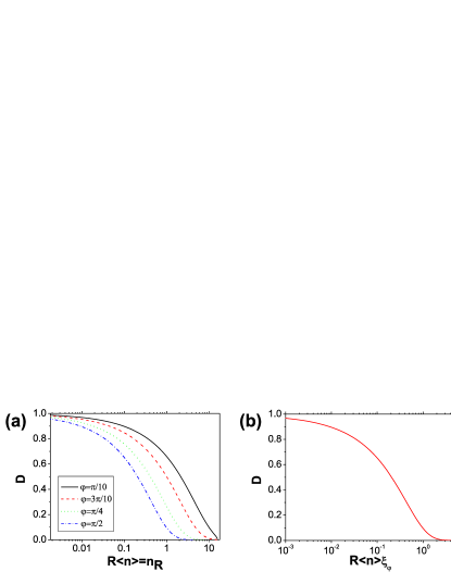
Figure 21: (a) Analytical results of the Bures distance for the superposition of coherent states, with $\alpha=4$ and for different values of the phase, as function of the average number of reflected photons. (b) Universal curve of the Bures distance for the superposition of coherent states for any $\alpha$ and $\varphi$, obtained by plotting eq.(106) as a function of the parameter $x=R\langle n\rangle\xi_{\varphi}$, with $\xi_{\varphi}=\sin^{2}\varphi$.

For $\varphi=\frac{\pi}{2}$, the coherent states exhibit opposite phases. Such condition represents the limit situation, in which the loss of coherence is higher since $\sin^{2}\varphi=1$. We observe, as is shown by fig.21, that the value of $D$ is reduced down to $\sim 0.1$ once $R|\alpha|^{2}=R\langle n\rangle=1$. Hence, the loss on the average of a single photon cancels most of the coherence in the quantum superposition state.

VII.3 Bures distance for QI-OPA amplified states

As a following step, we have evaluated numerically the distinguishability of $\left\{|\Phi^{+,-}\rangle\right\}$ through the distance $D(|\Phi^{+}\rangle,|\Phi^{-}\rangle)$ between the multiphoton states generated by QI-OPA. It is found that this property of $\left\{|\Phi^{+,-}\rangle\right\}$ coincides with the MQS Visibility of $|\Psi^{\pm}\rangle$, in virtue of the phase-covariance of the process: $D(|\Psi^{+}\rangle,|\Psi^{-}\rangle)$ = $D(|\Phi^{R}\rangle,|\Phi^{L}\rangle)$= $D(|\Phi^{+}\rangle,|\Phi^{-}\rangle)$. The visibility of the MQS $\left\{|\Psi^{+,-}\rangle\right\}$ has been evaluated numerically analyzing the Bures distance as a function of the average lost photons: $x\equiv R<n>$. This calculation have been performed by taking the complete expression of the density matrix, reported in Section IV and Appendices A-B, and by performing an approximate calculation of the fidelity through numerical algebraic matrix routines. This algorithm has been tested by evaluating numerically the Bures distance between the quantum superposition of coherent states $|\alpha\rangle\pm|-\alpha\rangle$. The comparison with the analytical result of Eq.(106) gave a high confidence level for the approximate results. The results for different values of the gain for equatorial macroqubits are reported in Fig.22 -(a).

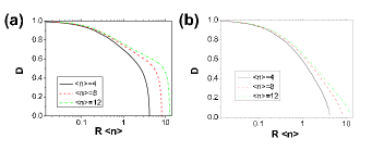
Figure 22: (a) Numerical evaluation of the distance $D(x)$ between two orthogonal equatorial macro-qubits $|\Phi^{\phi,\phi_{\bot}}\rangle$ as function of the average lost particle $x=R<n>$. Black straight line refers to $g=0.8$ and hence to $\langle n\rangle\approx 4$, red dashed line to $g=1.1$ and $\langle n\rangle\approx 8$, green dash-dotted line to $g=1.3$ and $\langle n\rangle\approx 12$. (b) Numerical evaluation of the distance $D(x)$ between two orthogonal linear macro-qubits $|\Phi^{H,V}\rangle$ as function of the average lost particle $x=R<n>$. Black straight line refers to $g=0.8$ and hence to $\langle n\rangle\approx 4$, red dashed line to $g=1.1$ and $\langle n\rangle\approx 8$, green dash-dotted line to $g=1.3$ and $\langle n\rangle\approx 12$.

Note that for small values of $x$ the decay of $D(x)$ is far slower than for the coherent state case shown in Fig.21- (b). Furthermore, after a common inflection point at $D\sim 0.6$ the slope of all functions $D(x)$ corresponding to different values of $<n>$ increases fast towards the infinite value, for increasing $\ x\rightarrow<n>$ and: $R\rightarrow 1$. The latter property can be demonstrated with a perturbative approach on the density matrix. We find, in the low $T$ and high gain limit of $\frac{\partial D(\hat{\rho}^{T}_{\varphi},\hat{\rho}^{T}_{\varphi_{\bot}})}{\partial T}$, the slope: $\lim_{g\rightarrow\infty}\lim_{T\rightarrow 0}\frac{\partial D(\hat{\rho}^{T}_{\varphi},\hat{\rho}^{T}_{\varphi_{\bot}})}{\partial T}=\lim_{g\rightarrow\infty}(1+4C^{2}+2C^{2}\Gamma(1+2\Gamma^{2})^{\frac{1}{2}})=\infty$. For total particle loss, $R$ = $1$ and $x$ = $<n>$ is: $D(x)$ = $0$. All this means that the MQS Visibility can be significant even if the average number $x$ of lost particles is very close to the initial total number $<n>$, i.e. for $R\sim 1$. This behavior is opposite to the case of coherent states where the function $D(R|\alpha|^{2})$ approaches the zero value with a slope equal to zero: Fig.21-(b).

For sake of completeness, we then performed the same calculation for the linear macroqubits $|\Phi^{H,V}\rangle$, and the results are reported in Fig.22-(b). For this injected qubit, not lying in the equatorial plane of the Bloch sphere, the amplification process does not correspond to an ”optimal cloning machine”. For this reason, the flow of noise from the enviroment in the amplification stage is not the minimum optimal value, and hence the output states possess a faster decoherence rate. Indeed, the output distributions, as shown in Fig.10-(b), do not possess the strong unbalancement in polarization of the equatorial macroqubits $|\Phi^{\varphi}\rangle$ that is responsible of their resilience structure.

VII.4 Distinguishability enhancement through an Orthogonality-Filter

As a further investigation, we consider the case of a more sophisticated measurement scheme based on an electronic device named O-Filter (OF). The demonstration of microscopic-macroscopic entanglement by adopting the O-Filter based measurement strategy was reported in DeMa08 . The POVM like technique Pere95 implied by this device locally selects, after an intensity measurement the events for which the difference between the photon numbers associated with two orthogonal polarizations $|n_{\pi}-m_{\pi_{\bot}}|>k$, i.e. larger than an adjustable threshold $k$ Naga07 , where $n_{\pi}$ is the number of photon polarized $\pi$ and $m_{\pi_{\bot}}$ the number of photon polarized $\pi_{\bot}$. By this method a sharper discrimination between the output states $|\Phi^{\varphi}\rangle$ and $|\Phi^{\varphi_{\bot}}\rangle$ can be achieved. The action of the OF, sketched in Fig.1 can be formalized through the POVM elements:

$$\hat{F}^{(+1)}_{\pi,\pi_{\bot}}(k) = \sum_{n=k}^{\infty}\sum_{m=0}^{n-k}\hat{\Pi}_{n,m}$$ (107)

$$\hat{F}^{(-1)}_{\pi,\pi_{\bot}}(k) = \sum_{m=k}^{\infty}\sum_{n=0}^{m-k}\hat{\Pi}_{n,m}$$ (108)

$$\hat{F}^{(0)}_{\pi,\pi_{\bot}}(k) = \hat{I}-\hat{F}^{(+1)}_{\pi}-\hat{F}^{(-1)}_{\pi}$$ (109)

where the $\hat{\Pi}_{n,m}=|n\pi,m\pi_{\bot}\rangle\,\langle n\pi,m\pi_{\bot}|$ are Fock-state Von-Neumann projectors that describe the performed intensity measurement. The average of the couple of operators $\langle\hat{F}^{(-1)}_{\pi,\pi_{\bot}}(k)\rangle+\langle\hat{F}^{(+1)}_{\pi,\pi_{\bot}}(k)\rangle$ defines the success probability of the O-Filter, i.e. the rate of events leading to one of the conclusive outcomes ($\pm 1$). To calculate the action of the O-Filter in the Bures distance, we projected the density matrix of the states over the joint subset corresponding to the ($\pm 1$) outcomes, neglecting only the terms leading to the inconclusive (0) result. Then, the same numerical analysis of the previous section has been performed. In Fig.23-(a) the results for $g=0.8$ and different values of $k$ are reported. Note the increase of the value of $D(x)$, i.e. of the MQS Visibility, by increasing $k$. Of course, the increase in the MQS Visibility through the O-Filter device is achieved at the cost of a lower success probability (Fig.23-(a)). According to the graphical analysis of Section IV on the photon number distributions of the equatorial amplified macro-states, the O-Filter device improves the MQS Visibility since it exploits the peculiar unbalancement in polarization of the equatorial amplified macro-states in a Fock-space analysis. In the selected regions, the $\left\{|\Phi^{\varphi}\rangle,|\Phi^{\varphi_{\bot}}\rangle\right\}$ states can be discriminated with a higher fidelity. As a further analysis, we reported in fig.23-(b) the trend of the success probability as a function of the threshold $k$ for different values of the transmittivity. Interestingly enough, we note that the success probability depends only on the ratio between the threshold $k$ and the number of transmitted photons $T\langle n\rangle$, since the three curves for different $T$ are almost superimposed. This is a consequence of the property of the photon number distribution of the equatorial macro-qubits, since its form is almost left unaltered after the propagation over a lossy channel.

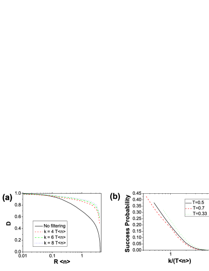
Figure 23: (a) Numerical evaluation of the Bures distance between two orthogonal equatorial macro-qubits after discrimination with the O-Filter for different values of the threshold $k$ ($g=0.8$). The filtering probabilities for the three cases are respectively $P(k=4T\langle n\rangle)=1.6*10^{-3}$, $P(k=6T\langle n\rangle)=7.14*10^{-5}$ and $P(k=8T\langle n\rangle)=3.06*10^{-6}$. (b) Success probability for the O-Filter for $g=0.8$ and different values of the transmittivity as a function of the parameter $\frac{k}{T\langle n\rangle}$. The latter expresses the threshold $k$ with respect to the average number of the incident photons in the detection apparatus. We note that the curves for different transmittivities can be almost superimposed.

VIII Wigner function for non-degenerate quantum injected optical parametric amplifier in the EPR configuration

In this section we derive the Wigner function associated to the non-degenerate quantum injected optical parametric amplifier, working in a non-collinear EPR configuration. The scheme for this device is reported in fig.24.

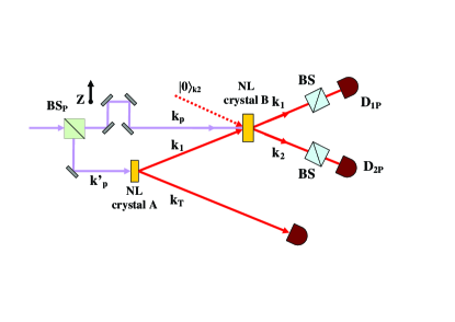
Figure 24: Scheme for the non-collinear optical parametric amplification of a single-photon state. An EPR pair is generated in a first non-linear crystal. The photon on mode $\mathbf{k}_{T}$ acts as a trigger to conditionally prepare the photon on mode $\mathbf{k}_{1}$. The latter is superimposed with a strong $\mathbf{k}_{P}$ pump beam, and is amplified in a second non-linear crystal oriented in the same optical configuration of the EPR source. The beam-splitters on modes $\mathbf{k}_{1}$ and $\mathbf{k}_{2}$ in the figure represent the lossy transmission channel.

In the stimulated regime, this amplifier acts as an $N\rightarrow M$ universal optimal quantum cloning machine Pell03 ; DeMa04 . The interaction Hamiltonian of this device can be written in the form:

$$\hat{\mathcal{H}}_{epr}=\imath\hbar\chi\left(\hat{a}_{1\pi}^{{\dagger}}\hat{a}_{2\pi_{\bot}}^{{\dagger}}-\hat{a}_{1\pi_{\bot}}^{{\dagger}}\hat{a}_{2\pi}^{{\dagger}}\right)+\mathrm{h.c.}$$ (110)

where $\pi$ stands for any polarization state, and $i=1,2$ for the two spatial modes. The time evolution of the field operators can be directly derived by the Heisenberg equations, obtaining:

$$\hat{a}_{1\pi(2\pi_{\bot})}^{{\dagger}}(t) = \hat{a}_{1\pi(2\pi_{\bot})}^{{\dagger}}C+\hat{a}_{2\pi_{\bot}(1\pi)}S$$ (111)

$$\hat{a}_{1\pi_{\bot}(2\pi)}^{{\dagger}}(t) = \hat{a}_{1\pi_{\bot}(2\pi)}^{{\dagger}}C-\hat{a}_{2\pi(1\pi_{\bot})}S$$ (112)

In the following paragraphs we shall proceed with the calculation of the Wigner function for this amplifier in the stimulated regime, i.e. when a generic Fock-state is injected on the spatial mode $\mathbf{k}_{1}$.

VIII.1 Wigner function for the non-collinear QIOPA in absence of decoherence

In this section we derive the Wigner function for the QIOPA in a non collinear configuration. Without loss of generality, let us restrict our attention to the equatorial polarization basis $\vec{\pi}_{\varphi}=\frac{1}{\sqrt{2}}\left(\vec{\pi}_{H}+e^{\imath\varphi}\vec{\pi}_{V}\right)$ and $\vec{\pi}_{\varphi_{\bot}}=\frac{1}{\sqrt{2}}\left(-e^{-\imath\varphi}\vec{\pi}_{H}+\vec{\pi}_{V}\right)$. As for the collinear case, the injected state over spatial mode $\mathbf{k}_{1}$ is the generic Fock-state $|\psi_{in}\rangle_{12}=|N\varphi,M\varphi_{\bot}\rangle_{1}\otimes|0\varphi,0\varphi_{\bot}\rangle_{2}$. The characteristic function is then evaluated starting from the definition:

$$\chi_{N,M}\left\{\eta,\xi,t\right\} =\,_{12}\langle\psi_{in}|e^{\eta_{1}\hat{a}_{1H}^{{\dagger}}(t)-\eta_{1}^{\ast}\hat{a}_{1H}(t)}e^{\eta_{2}\hat{a}_{2V}^{{\dagger}}(t)-\eta_{2}^{\ast}\hat{a}_{2V}(t)}$$ (113)

$$e^{\xi_{1}\hat{a}_{1V}^{{\dagger}}(t)-\xi_{1}^{\ast}\hat{a}_{1V}(t)}e^{\xi_{2}\hat{a}_{2H}^{{\dagger}}(t)-\xi_{2}^{\ast}\hat{a}_{2H}(t)}|\psi_{in}\rangle_{12}$$

Let us apply the transformation $\left\{\eta,\xi\right\}\rightarrow\left\{\overline{\eta}(t),\overline{\xi}(t)\right\}$, where:

$$\overline{\eta}_{1}=\frac{1}{\sqrt{2}}\left(\eta_{1}+e^{-\imath\varphi}\xi_{1}\right) \overline{\xi}_{1}=\frac{1}{\sqrt{2}}\left(-e^{\imath\varphi}\eta_{1}+\xi_{1}\right)$$ ; (114)

$$\overline{\eta}_{2}=\frac{1}{\sqrt{2}}\left(\eta_{2}-e^{\imath\varphi}\xi_{2}\right) \overline{\xi}_{2}=\frac{1}{\sqrt{2}}\left(e^{-\imath\varphi}\eta_{2}+\xi_{2}\right)$$ ; (115)

and:

$$\overline{\eta}_{1(2)}(t) = \overline{\eta}_{1(2)}C-\overline{\eta}_{2(1)}^{\ast}S$$ (116)

$$\overline{\xi}_{1(2)}(t) = \overline{\xi}_{1(2)}C+\overline{\xi}_{2(1)}^{\ast}S$$ (117)

With analogous calculation to the one performed in Section III we obtain:

$$\chi_{N,M}\left\{\eta,\xi,t\right\} =\exp\left[-\frac{1}{2}\sum_{j=1}^{2}\left(|\overline{\eta}_{j}(t)|^{2}+|\overline{\xi}_{j}(t)|^{2}\right)\right]$$ (118)

$$\times\left(\sum_{n=0}^{N}\frac{N!(-1)^{n}}{(N-n)!n!^{2}}|\overline{\eta}_{1}(t)|^{2n}\right)$$

$$\times\left(\sum_{m=0}^{M}\frac{M!(-1)^{m}}{(M-m)!m!^{2}}|\overline{\xi}_{1}(t)|^{2m}\right)$$

The Wigner function of the amplified field can be then expressed as the 8-dimensional Fourier transform of the characteristic function, according to its definition. By inserting the explicit expression of the characteristic function, by separating the integrals on each couple of complex conjugate variables, and by exploiting the integral relations already used in sec.III we find:

$$W {}_{|N\varphi,M\varphi_{\bot}\rangle}\left\{\alpha,\beta,t\right\}=\left(\frac{2}{\pi}\right)^{4}(-1)^{N+M}e^{-2|\Delta|^{2}}$$ (119)

$$L_{N}\left(|\Delta_{A}\left\{\alpha\right\}+e^{-\imath\varphi}\Delta_{B}\left\{\beta\right\}|^{2}\right)$$

$$L_{M}\left(|-\Delta_{A}\left\{\alpha\right\}e^{\imath\varphi}+\Delta_{B}\left\{\beta\right\}|^{2}\right)$$

The $\Delta_{A}\left\{\alpha\right\}$, $\Delta_{B}\left\{\beta\right\}$ and $|\Delta|^{2}$ variables are defined in Appendix C, where all the details of the calculation of the Wigner function are reported.

Let us we consider the injection of a single photon with polarization state $|\varphi\rangle_{1}=\frac{1}{\sqrt{2}}\left(|H\rangle+e^{\imath\varphi}|V\rangle\right)$. The Wigner function reads DeMa98 :

$$W_{|1\varphi,0\varphi_{\bot}\rangle}\left\{\alpha,\beta,t\right\}=\frac{16}{\pi^{4}}e^{-2|\Delta|^{2}}(|\Delta_{A}\left\{\alpha\right\}+e^{-\imath\varphi}\Delta_{B}\left\{\beta\right\}|^{2}-1)$$ (120)

where $|\Delta_{A}\left\{\alpha\right\}+e^{-\imath\varphi}\Delta_{B}\left\{\beta\right\}|^{2}$ represents the interference term due to the quantum superposition form of the input state. Indeed this interference term defines a phase-space region where the Wigner function is negative, showing the broadcasting of the quantum properties of the injected single photon state to the amplified field. For more details on the amplification of a single photon, refer to DeMa98 .

VIII.2 Wigner function for the non-collinear EPR optical parametric amplifier in presence of decoherence

In this section we are interested in the Wigner function for the non-degenerate optical parametric amplifier in presence of losses. The lossy channels on the two spatial modes $\left\{\mathbf{k}_{1},\mathbf{k}_{2}\right\}$ are again simulated by a beam-splitter model, with input-output relations:

$$\hat{c}^{{\dagger}}_{i}=\sqrt{T}\hat{a}_{i}(t)+\imath\sqrt{R}\hat{b}_{i}$$ (121)

where a vacuum state is injected in the $\hat{b}_{i}$ ports of the beam-splitters. We considered the case of two transmission channels for modes $\mathbf{k}_{1}$ and $\mathbf{k}_{2}$ with equal efficiencies.

The characteristic function is then evaluated as:

$$\chi_{N,M}\left\{\eta,\xi,R,t\right\}=\,_{AB}\langle\psi_{in}|e^{\overline{\eta}_{1}\hat{a}_{1\varphi}^{{\dagger}}(t)-\overline{\eta}_{1}^{\ast}\hat{a}_{1\varphi}(t)}e^{\overline{\eta}_{2}\hat{a}_{2\varphi_{\bot}}^{{\dagger}}(t)-\overline{\eta}_{2}^{\ast}\hat{a}_{2\varphi_{\bot}}(t)}e^{\overline{\xi}_{1}\hat{a}_{1\varphi_{\bot}}^{{\dagger}}(t)-\overline{\xi}_{1}^{\ast}\hat{a}_{1\varphi_{\bot}}(t)}e^{\overline{\xi}_{2}\hat{a}_{2\varphi}^{{\dagger}}(t)-\overline{\xi}_{2}^{\ast}\hat{a}_{2\varphi}(t)}|\psi_{in}\rangle_{AB}$$ (122)

The transformation to the $\left\{\overline{\eta},\overline{\xi}\right\}$ variables is the same as in the unperturbed case, and has been defined previously in Eqq.(114-115). Following the approach of Section VIII, we insert the beam-splitter relations (121) and evaluate the averages after writing the exponential operators in normally ordered form. We obtain:

$$\chi_{N,M} \left\{\eta,\xi,R,t\right\}=\exp\left[-\frac{1}{2}\left(1+2RS^{2}\right)\sum_{j=1}^{2}\left(|\overline{\eta}_{j}(t)|^{2}+|\overline{\xi}_{j}(t)|^{2}\right)\right]\exp\left[-RCS\left(\overline{\eta}_{1}(t)\overline{\eta}_{2}(t)+\overline{\eta}_{1}^{\ast}(t)\overline{\eta}_{2}^{\ast}(t)\right)\right]$$ (123)

$$\times\exp\left[RCS\left(\overline{\xi}_{1}(t)\overline{\xi}_{2}(t)+\overline{\xi}_{1}^{\ast}(t)\overline{\xi}_{2}^{\ast}(t)\right)\right]\left(\sum_{n=0}^{N}\frac{N!(-T)^{n}}{(N-n)!n!^{2}}|\overline{\eta}_{1}(t)|^{2n}\right)\left(\sum_{m=0}^{M}\frac{M!(-T)^{m}}{(M-m)!m!^{2}}|\overline{\xi}_{1}(t)|^{2m}\right)$$

The Wigner function of the field can then be evaluated as the 8-dimensional Fourier transform:

$$W_{|N\varphi,M\varphi_{\bot}\rangle}\left\{\alpha,\beta,R,t\right\} =\frac{1}{\pi^{8}}\int\int\int\int\left(\prod_{j=1}^{2}d^{2}\overline{\eta}_{j}d^{2}\overline{\xi}_{j}\right)\chi_{N,M}\left\{\eta,\xi,R,t\right\}\exp\left\{\sum_{j=1}^{2}\left[\overline{\eta}^{\ast}_{j}(t)\overline{\alpha}_{j}(t)-\overline{\eta}_{j}(t)\overline{\alpha}^{\ast}_{j}(t)\right]\right\}$$ (124)

$$\times\exp\left\{\sum_{j=1}^{2}\left[\overline{\xi}^{\ast}_{j}(t)\overline{\beta}_{j}(t)-\overline{\xi}_{j}(t)\overline{\beta}^{\ast}_{j}(t)\right]\right\}$$

After the explicit insertion of the characteristic function, the Wigner function can be written as a product of two integrals:

$$W_{|N\varphi,M\varphi_{\bot}\rangle}\left\{\alpha,\beta,R,t\right\}=I^{+}_{N}\left\{\alpha,R,t\right\}I_{M}^{-}\left\{\beta,R,t\right\}$$ (125)

where the $I_{N}^{+}\left\{\alpha,R,t\right\}$ and $I_{M}^{-}\left\{\alpha,R,t\right\}$ are:

$$I^{+}_{N}\left\{\alpha,R,t\right\} = \frac{1}{\pi^{2}}\sum_{n=0}^{N}d_{n}^{N}(T)J_{n,0}\left(\varepsilon^{{}^{\prime}},\mu;\overline{\alpha}_{1}(t),\overline{\alpha}_{2}(t)\right)$$ (126)

$$I^{-}_{M}\left\{\beta,R,t\right\} = \frac{1}{\pi^{2}}\sum_{m=0}^{M}d_{m}^{M}(T)J_{m,0}\left(\varepsilon^{{}^{\prime}},-\mu;\overline{\beta}_{1}(t),\overline{\beta}_{2}(t)\right)$$ (127)

The $J_{n,0}$ integrals are explicited in Appendix A in Eq.(170). The parameters $\varepsilon^{{}^{\prime}},\mu,d_{n}^{N}(T)$ for the non-collinear optical parametric amplifier are:

$$d_{n}^{N}(T) = \begin{pmatrix}N\\ n\end{pmatrix}\frac{(-T)^{n}}{n!}$$ (128)

$$\varepsilon^{{}^{\prime}} = \frac{1}{2}\left(1+2RS^{2}\right)$$ (129)

$$\mu = RCS$$ (130)

Let us again focus on the single-photon case, corresponding to $N=1$ and $M=0$. With an analogous procedure to the collinear case, we analyze the persistence of negative regions in the Wigner function after the decoherence process. Analyzing the form of Eq.(120), we note that the minimum occurs when $|\Delta_{A}\left\{\alpha\right\}+e^{-\imath\varphi}\Delta_{B}\left\{\beta\right\}|^{2}=0$ and $|\Delta|^{2}=0$. This point corresponds to the origin of the 8-dimensional phase space given by the $\left\{\overline{\alpha}(t),\overline{\beta}(t)\right\}$ variables. The evolution of the Wigner function in this point is explicitly evaluated as:

$$W_{|1\varphi,0\varphi_{\bot}\rangle}\left\{0,0,R,t\right\}=\frac{16}{\pi^{4}}\frac{2R-1}{\left[1+4R(1-R)S^{2}\right]^{3}}$$ (131)

The value in the origin of the Wigner function is reported in Fig. 25. We note an analogous trend with respect to the collinear case, while the absolute value of the amount of negativity is smaller. This is due to the universal cloning feature of the non-collinear QI-OPA, in which the cloning fidelity is smaller than the one in phase-covariant case.

We conclude this Section on the non-collinear QI-OPA by stressing that a full phase-space characterization of the quantum states generated by this device would require a couple of double homodyne measurement setups, one for each spatial mode, as the one discussed in Section III.3.

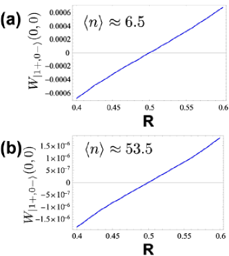
Figure 25: Transition from a non-positive distribution to a completely positive Wigner function of the single-photon amplified states, obtained by the non-collinear QI-OPA in presence of decoherence, as a function of the beam-splitter reflectivity $R$. Average photon number of (a) $\langle n\rangle\approx 6.5$ and (b) $\langle n\rangle\approx 53.5$. The negativity is evaluated as the value of the Wigner function in the origin.

IX Conclusion and perspectives

The quantum properties of the QI-OPA generated macroscopic system, have been investigated in phase-space by a Wigner quasi-probability function analysis when this class of states is transmitted over a lossy channel, i.e. in presence of a decohering system - enviroment interaction which represents the main limitation in the implementation of quantum information tasks. We first considered the ideal case, in absence of losses, showing the presence of peculiar quantum properties such as squeezing and a non-positive W-representation. Then, after a brief review of the properties of the coherent states MQS, the resilience to losses of QI-OPA amplified states in a lossy configuration was investigated, allowing to observe the persistence of the non-positivity of the Wigner function in a certain range of the system-enviroment interaction parameter $R$. This behaviour was analyzed in close comparison with the $|\alpha\rangle$ states MQS, which possesses a non-positive W-representation in the same interval of the interaction parameter $R$. Moreover, the more resilient structure of the QI-OPA amplified states was emphasized by their slower decoherence rate, represented by both the slower decrease in the negative part of the Wigner function and by the behavior of the Bures distance between orthogonal macrostates, the latter evaluated in the Fock-Space. Since the negativity of the W-representation is a sufficent but not a necessary condition for the non-classicality of any physical system, future investigations could be aimed to the analysis of the decoherence regime in which the Wigner function is completely positive, analyzing the presence of quantum properties from a different point of view.

We acknowledge useful discussions with Wolfgang Schleich. Work supported by PRIN 2005 of MIUR and INNESCO 2006 of CNISM.

Appendix A Density matrix of the equatorial amplified states after the propagation over a lossy channel

In this appendix we perform the derivation of the density matrix of the equatorial amplified states after the propagation over a lossy channel. The applied model is the same BS-scattering process used throughout the whole paper.

The starting point is the expression of the unperturbed state $|\Phi^{\varphi}\rangle{}$:

$$|\Phi^{\varphi}\rangle{} =\frac{1}{C^{2}}\sum_{i,j=0}^{\infty}\left(e^{-\imath\varphi}\frac{\Gamma}{2}\right)^{i}\left(-e^{\imath\varphi}\frac{\Gamma}{2}\right)^{j}$$ (132)

$$\times\frac{\sqrt{(2i+1)!}\,\sqrt{2j!}}{i!\,j!}|(2i+1)\varphi,(2j)\varphi_{\bot}\rangle{}$$

where $C=\cosh g$ and $\Gamma=\tanh g$, with $g$ gain of the amplifier, with the state written in the polarization basis $\left\{\vec{\pi}_{\varphi},\vec{\pi}_{\varphi_{\bot}}\right\}$. The state can be written in terms of the creation operators:

$$|\Phi^{\varphi}\rangle{}=\frac{1}{C^{2}}\sum_{i,j=0}^{\infty}\left(e^{-\imath\varphi}\frac{\Gamma}{2}\right)^{i}\left(-e^{\imath\varphi}\frac{\Gamma}{2}\right)^{j}\frac{\left(\hat{a}_{\varphi}^{{\dagger}}\right)^{2i+1}\,\left(\hat{a}_{\varphi_{\bot}}^{{\dagger}}\right)^{2j}}{i!\,j!}|0\rangle{}$$ (133)

We then apply the time evolution independent operators $\hat{U}_{BS}^{(\varphi)}$ and $\hat{U}_{BS}^{(\varphi_{\bot})}$, which describe the interaction in the beam-splitter: $\hat{U}_{BS}=e^{\imath\frac{\theta}{2}\left(\hat{a}^{{\dagger}}\hat{b}+\hat{a}\hat{b}^{{\dagger}}\right)}$. As a reasonable assumption, we consider the transmittivity $T_{\varphi}$ and $T_{\varphi_{\bot}}$ to be equal for all polarization states. We can then write the evolved state in the Schrodinger picture $|\Phi^{{}^{\prime}\varphi}\rangle$ as:

$$|\Phi^{\prime\varphi}\rangle{} =\hat{U}_{BS}^{(\varphi)}\hat{U}_{BS}^{(\varphi_{\bot})}|\Phi^{\varphi}\rangle{}=\frac{1}{C^{2}}\sum_{i,j=0}^{\infty}\left(e^{-\imath\varphi}\frac{\Gamma}{2}\right)^{i}\left(-e^{\imath\varphi}\frac{\Gamma}{2}\right)^{j}$$ (134)

$$\times\frac{\left(\sqrt{T}\hat{c}_{\varphi}^{{\dagger}}+\imath\sqrt{R}\hat{d}_{\varphi}^{{\dagger}}\right)^{2i+1}\,\left(\sqrt{T}\hat{c}_{\varphi_{\bot}}^{{\dagger}}+\imath\sqrt{R}\hat{d}_{\varphi_{\bot}}^{{\dagger}}\right)^{2j}}{i!\,j!}|0\rangle{}$$

We can now exploit the binomial expansion $(a+b)^{n}=\sum_{i=0}^{n}a^{i}b^{n-i}\begin{pmatrix}n\\ i\end{pmatrix}$, as the operators for the two output mode of the beam-splitter $\hat{c},\hat{d}$ commute and can be treated as algebraic variables. Subsequently applying the creation operators to the vacuum we then obtain the final expression of the state after the propagation in the beam-splitter:

$$|\Phi^{\prime\varphi}\rangle{} =\frac{1}{C^{2}}\sum_{i,j=0}^{\infty}\left(e^{-\imath\varphi}\frac{\Gamma}{2}\right)^{i}\left(-e^{\imath\varphi}\frac{\Gamma}{2}\right)^{j}$$ (135)

$$\times\sum_{m=0}^{2i+1}\sum_{n=0}^{2j}\left[\begin{pmatrix}2i+1\\ m\end{pmatrix}\begin{pmatrix}2j\\ n\end{pmatrix}\right]^{\frac{1}{2}}\frac{\sqrt{(2i+1)!}\,\sqrt{2j!}}{i!\,j!}$$

$$\times\left(\sqrt{T}\right)^{n+m}\left(\imath\sqrt{R}\right)^{2i+2j+1-n-m}$$

$$\times|m,n\rangle_{C}\otimes|2i+1-m,2j-n\rangle_{D}$$

The density matrix of the quantum state is then obtained as $\hat{\rho^{\prime}}^{\varphi}=|\Phi^{\prime}{}^{\varphi}\rangle\langle\Phi^{\prime}{}^{\varphi}|$. Let us call:

$$\gamma_{ij,mn} =\frac{1}{C^{2}}\left(e^{-\imath\varphi}\frac{\Gamma}{2}\right)^{i}\left(-e^{\imath\varphi}\frac{\Gamma}{2}\right)^{j}\left[\begin{pmatrix}2i+1\\ m\end{pmatrix}\begin{pmatrix}2j\\ n\end{pmatrix}\right]^{\frac{1}{2}}$$ (136)

$$\times\frac{\sqrt{(2i+1)!}\,\sqrt{2j!}}{i!\,j!}\left(\sqrt{T}\right)^{n+m}\left(\imath\sqrt{R}\right)^{2i+2j+1-n-m}$$

Tracing the density matrix $\hat{\rho^{\prime}}^{\varphi}$ on the reflected $\hat{d}$ BS-mode in order to consider our ignorance over the number of reflected photons we obtain:

$$\hat{\rho}_{T}^{\varphi} =\mathrm{Tr}_{D}\left(\hat{\rho^{\prime}}^{\varphi}\right)=\sum_{x,y=0}^{\infty}\,{}_{D}\langle x,y|\Phi^{\prime\varphi}\rangle\,\langle\Phi^{\prime\varphi}|x,y\rangle_{D}=$$ (137)

$$=\sum_{x,y=0}^{\infty}\sum_{i,j,k,l=0}^{\infty}\sum_{m=0}^{2i+1}\sum_{n=0}^{2j}\sum_{p=0}^{2k+1}\sum_{q=0}^{2l}\gamma_{ij,mn}\gamma^{\ast}_{kl,pq}|m,n\rangle\,\langle p,q|$$

$$\otimes\,_{D}\langle x,y|2i+1-m,2j-n\rangle_{D}\,{}_{D}\langle 2k+1-p,2l-q|x,y\rangle_{D}$$

The evaluation of the scalar products between Fock-states lead to the desired result. The expression of the density matrix on the transmitted $\hat{c}$ spatial BS-mode is then written in the form:

$$\hat{\rho}_{T}^{\varphi}=\sum_{i,j,k,q=0}^{\infty}\,\langle i,j|\hat{\rho}_{T}^{\varphi}|k,q\rangle\,|i,j\rangle\,\langle k,q|$$ (138)

We now report the expressions of the density matrix coefficients, which depend on the parity. For $i,j,k,q$ even we obtain:

$$\langle i,j|\hat{\rho}^{\varphi}_{T}|k,q\rangle =\frac{1}{C^{4}}\left(\frac{\Gamma}{2}\right)^{\frac{i+k}{2}}\left(-\frac{\Gamma}{2}\right)^{\frac{j+q}{2}}\left(e^{\imath\varphi}\right)^{\frac{j+k-i-q}{2}}R\left(\sqrt{T}\right)^{i+j+k+q}\frac{\sqrt{i!j!k!q!}}{\frac{i}{2}!\frac{j}{2}!\frac{k}{2}!\frac{q}{2}!}(i+1)(k+1)$$ (139)

$$\left[\frac{1}{1-R^{2}\Gamma^{2}}\right]^{2+\frac{i+j+k+q}{2}}\,_{2}F_{1}\left(-\frac{i}{2},-\frac{k}{2};\frac{3}{2};R^{2}\Gamma^{2}\right)\,_{2}F_{1}\left(-\frac{j}{2},-\frac{q}{2};\frac{1}{2};R^{2}\Gamma^{2}\right)$$

For $i,k$ odd and $j,q$ even, we obtain:

$$\langle i,j|\hat{\rho}^{\varphi}_{T}|k,q\rangle =\frac{1}{C^{4}}\left(\frac{\Gamma}{2}\right)^{\frac{i+k}{2}-1}\left(-\frac{\Gamma}{2}\right)^{\frac{j+q}{2}}\left(e^{\imath\varphi}\right)^{\frac{j+k-i-q}{2}}\left(\sqrt{T}\right)^{i+j+k+q}\frac{\sqrt{i!j!k!q!}}{\frac{i-1}{2}!\frac{j}{2}!\frac{k-1}{2}!\frac{q}{2}!}$$ (140)

$$\left[\frac{1}{1-R^{2}\Gamma^{2}}\right]^{2+\frac{i+j+k+q}{2}}\,_{2}F_{1}\left(-\frac{1+i}{2},-\frac{1+k}{2};\frac{1}{2};R^{2}\Gamma^{2}\right)\,_{2}F_{1}\left(-\frac{j}{2},-\frac{q}{2};\frac{1}{2};R^{2}\Gamma^{2}\right)$$

For $i,k$ even and $j,q$ odd, we obtain:

$$\langle i,j|\hat{\rho}^{\varphi}_{T}|k,q\rangle =\frac{1}{C^{4}}\left(\frac{\Gamma}{2}\right)^{\frac{i+k}{2}}\left(-\frac{\Gamma}{2}\right)^{\frac{j+q}{2}-1}\left(e^{\imath\varphi}\right)^{\frac{j+k-i-q}{2}}R^{2}\Gamma^{2}\left(\sqrt{T}\right)^{i+j+k+q}(i+1)(k+1)\frac{\sqrt{i!j!k!q!}}{\frac{i}{2}!\frac{j-1}{2}!\frac{k}{2}!\frac{q-1}{2}!}$$ (141)

$$\left[\frac{1}{1-R^{2}\Gamma^{2}}\right]^{2+\frac{i+j+k+q}{2}}\,_{2}F_{1}\left(-\frac{i}{2},-\frac{k}{2};\frac{3}{2};R^{2}\Gamma^{2}\right)\,_{2}F_{1}\left(\frac{1-j}{2},\frac{1-q}{2};\frac{3}{2};R^{2}\Gamma^{2}\right)$$

Finally, for $i,j,k,q$ odd we obtain:

$$\langle i,j|\hat{\rho}^{\varphi}_{T}|k,q\rangle =\frac{1}{C^{4}}\left(\frac{\Gamma}{2}\right)^{\frac{i+k}{2}-1}\left(-\frac{\Gamma}{2}\right)^{\frac{j+q}{2}-1}\left(e^{\imath\varphi}\right)^{\frac{j+k-i-q}{2}}R\Gamma^{2}\left(\sqrt{T}\right)^{i+j+k+q}\frac{\sqrt{i!j!k!q!}}{\frac{i-1}{2}!\frac{j-1}{2}!\frac{k-1}{2}!\frac{q-1}{2}!}$$ (142)

$$\left[\frac{1}{1-R^{2}\Gamma^{2}}\right]^{2+\frac{i+j+k+q}{2}}\,_{2}F_{1}\left(-\frac{1+i}{2},-\frac{1+k}{2};\frac{1}{2};R^{2}\Gamma^{2}\right)\,_{2}F_{1}\left(\frac{1-j}{2},\frac{1-q}{2};\frac{3}{2};R^{2}\Gamma^{2}\right)$$

In these expressions, ${}_{2}F_{1}\left(\alpha,\beta;\gamma;z\right)$ are Hyper-geometric functions Slat66 .

Appendix B Density matrix of the $\vec{\pi}_{H},\vec{\pi}_{V}$ amplified states after the propagation over a lossy channel

The procedure for the evaluation of the density matrix of the state after losses is the same applied in the previous section. Let us analyze the $|\Phi^{H}\rangle$ state, whose density matrix after the amplification process reads:

$$\hat{\rho}^{H} =|\Phi^{H}\rangle\,\langle\Phi^{H}|=\frac{1}{C^{4}}\sum_{n,m=0}^{\infty}\Gamma^{n+m}\sqrt{n+1}\sqrt{m+1}$$ (143)

$$|(n+1)H,nV\rangle\,\langle(m+1)H,mV|$$

After the insertion of the BS unitary transformation, the joint density matrix of the transmitted and reflected modes is:

$$\hat{\rho}^{{}^{\prime}H} =\frac{1}{C^{4}}\sum_{m,n=0}^{\infty}\sum_{i=0}^{n+1}\sum_{j=0}^{n}\sum_{k=0}^{m+1}\sum_{q=0}^{m}\Gamma^{n+m}\sqrt{n+1}\sqrt{m+1}$$ (144)

$$(-1)^{2m+1-k-q}\left[\begin{pmatrix}n+1\\ i\end{pmatrix}\begin{pmatrix}n\\ j\end{pmatrix}\begin{pmatrix}m+1\\ k\end{pmatrix}\begin{pmatrix}m\\ q\end{pmatrix}\right]^{\frac{1}{2}}$$

$$\left(\sqrt{T}\right)^{i+j+k+q}\left(\sqrt{R}\right)^{n+m+2-i-j-k-q}$$

$$|iH,jV\rangle_{C}\langle kH,qV|\otimes$$

$$\otimes|(n+1-i)H,(n-j)V\rangle_{D}\langle(m+1-k)H,(m-q)V|$$

After tracing over the reflected mode, we finally obtain:

$$\hat{\rho}^{H}_{T}=\sum_{i=1}^{\infty}\sum_{j=0}^{i-1}\sum_{k=0}^{\infty}\left(\sum_{p=0}^{\infty}\overline{\gamma}_{ijk;p}\right)|iH,jV\rangle\,\langle kH,(k+j-i)V|+$$ (145)

$$+\sum_{i=0}^{\infty}\sum_{j=i}^{\infty}\sum_{k=0}^{\infty}\left(\sum_{p=j+1-i}^{\infty}\overline{\gamma}_{ijk;p}\right)|iH,jV\rangle\,\langle kH,(k+j-i)V|$$

where the coefficients $\overline{\gamma}_{ijk;p}$ are:

$$\overline{\gamma}_{ijk;p} =\frac{\Gamma^{2p+i+k-2}}{C^{4}}\sqrt{p+i}\sqrt{p+k}\,T^{k+j}R^{2p+i-1-j}$$ (146)

$$\left[\begin{pmatrix}p+i\\ i\end{pmatrix}\begin{pmatrix}p+i-1\\ j\end{pmatrix}\begin{pmatrix}p+k\\ k\end{pmatrix}\begin{pmatrix}p+k-1\\ k+j-1\end{pmatrix}\right]^{\frac{1}{2}}$$

Appendix C Wigner function for the non collinear QI-OPA in absence of decoherence

We begin the calculation of the Wigner function, without loss of generality, by restricting our attention to the equatorial polarization basis, defined by:

$$\vec{\pi}_{\varphi} = \frac{1}{\sqrt{2}}\left(\vec{\pi}_{H}+e^{\imath\varphi}\vec{\pi}_{V}\right)$$ (147)

$$\vec{\pi}_{\varphi_{\bot}} = \frac{1}{\sqrt{2}}\left(-e^{-\imath\varphi}\vec{\pi}_{H}+\vec{\pi}_{V}\right)$$ (148)

As for the collinear case, the injected state over spatial mode $\mathbf{k}_{1}$ is the generic Fock-state $|\psi_{in}\rangle_{12}=|N\varphi,M\varphi_{\bot}\rangle_{1}\otimes|0\varphi,0\varphi_{\bot}\rangle_{2}$. The characteristic function is then evaluated starting from the definition:

$$\chi_{N,M}\left\{\eta,\xi,t\right\} =\,_{12}\langle\psi_{in}|e^{\eta_{1}\hat{a}_{1H}^{{\dagger}}(t)-\eta_{1}^{\ast}\hat{a}_{1H}(t)}e^{\eta_{2}\hat{a}_{2V}^{{\dagger}}(t)-\eta_{2}^{\ast}\hat{a}_{2V}(t)}$$ (149)

$$e^{\xi_{1}\hat{a}_{1V}^{{\dagger}}(t)-\xi_{1}^{\ast}\hat{a}_{1V}(t)}e^{\xi_{2}\hat{a}_{2H}^{{\dagger}}(t)-\xi_{2}^{\ast}\hat{a}_{2H}(t)}|\psi_{in}\rangle_{12}$$

Let us apply the following transformations over the $\left\{\eta,\xi\right\}$ variables, corresponding to the rotations from the $\left\{\vec{\pi}_{H},\vec{\pi}_{V}\right\}$ to the $\left\{\vec{\pi}_{\varphi},\vec{\pi}_{\varphi_{\bot}}\right\}$ polarization basis:

$$\overline{\eta}_{1} = \frac{1}{\sqrt{2}}\left(\eta_{1}+e^{-\imath\varphi}\xi_{1}\right)$$ (150)

$$\overline{\xi}_{1} = \frac{1}{\sqrt{2}}\left(-e^{\imath\varphi}\eta_{1}+\xi_{1}\right)$$ (151)

$$\overline{\eta}_{2} = \frac{1}{\sqrt{2}}\left(\eta_{2}-e^{\imath\varphi}\xi_{2}\right)$$ (152)

$$\overline{\xi}_{2} = \frac{1}{\sqrt{2}}\left(e^{-\imath\varphi}\eta_{2}+\xi_{2}\right)$$ (153)

We then explicitly insert the time evolution of the field operators (111-112). Defining:

$$\overline{\eta}_{1}(t) = \overline{\eta}_{1}C-\overline{\eta}_{2}^{\ast}S$$ (154)

$$\overline{\eta}_{2}(t) = \overline{\eta}_{2}C-\overline{\eta}_{1}^{\ast}S$$ (155)

$$\overline{\xi}_{1}(t) = \overline{\xi}_{1}C+\overline{\xi}_{2}^{\ast}S$$ (156)

$$\overline{\xi}_{2}(t) = \overline{\xi}_{2}C+\overline{\xi}_{1}^{\ast}S$$ (157)

we can re-write the characteristic function in the following form:

$$\chi_{N,M}\left\{\eta,\xi,t\right\} =\,_{12}\langle\psi_{in}|e^{\overline{\eta}_{1}(t)\hat{a}_{1\varphi}^{{\dagger}}-\overline{\eta}_{1}^{\ast}(t)\hat{a}_{1\varphi}}e^{\overline{\eta}_{2}(t)\hat{a}_{2\varphi_{\bot}}^{{\dagger}}-\overline{\eta}_{2}^{\ast}(t)\hat{a}_{2\varphi_{\bot}}}$$ (158)

$$e^{\overline{\xi}_{1}(t)\hat{a}_{1\varphi_{\bot}}^{{\dagger}}-\overline{\xi}_{1}^{\ast}(t)\hat{a}_{1\varphi_{\bot}}}e^{\overline{\xi}_{2}(t)\hat{a}_{2\varphi}^{{\dagger}}-\overline{\xi}_{2}^{\ast}(t)\hat{a}_{2\varphi}}|\psi_{in}\rangle_{12}$$

The averages can now be evaluated by writing the operators in the normally ordered form. With analogous calculation to the one performed in Section III we obtain:

$$\chi_{N,M}\left\{\eta,\xi,t\right\} =\exp\left[-\frac{1}{2}\sum_{j=1}^{2}\left(|\overline{\eta}_{j}(t)|^{2}+|\overline{\xi}_{j}(t)|^{2}\right)\right]$$ (159)

$$\times\left(\sum_{n=0}^{N}\frac{N!(-1)^{n}}{(N-n)!n!^{2}}|\overline{\eta}_{1}(t)|^{2n}\right)$$

$$\times\left(\sum_{m=0}^{M}\frac{M!(-1)^{m}}{(M-m)!m!^{2}}|\overline{\xi}_{1}(t)|^{2m}\right)$$

The Wigner function of the amplified field can be then expressed as the 8-dimensional Fourier transform of the characteristic function, according to its definition. The integration variables are changed according to $\left\{\eta_{j},\xi_{j}\right\}_{j=1}^{2}\rightarrow\left\{\overline{\eta}_{j}(t),\overline{\xi}_{j}(t)\right\}_{j=1}^{2}$, leading to:

$$W_{|N\varphi,M\varphi_{\bot}\rangle}\left\{\alpha,\beta,t\right\} =\frac{1}{\pi^{8}}\int\int\int\int\left(\prod_{j=1}^{2}d^{2}\overline{\eta}_{j}d^{2}\overline{\xi}_{j}\right)\chi_{N,M}\left\{\eta,\xi,t\right\}\exp\left\{\sum_{j=1}^{2}\left[\overline{\eta}^{\ast}_{j}(t)\overline{\alpha}_{j}(t)-\overline{\eta}_{j}(t)\overline{\alpha}^{\ast}_{j}(t)\right]\right\}$$ (160)

$$\exp\left\{\sum_{j=1}^{2}\left[\overline{\xi}^{\ast}_{j}(t)\overline{\beta}_{j}(t)-\overline{\xi}_{j}(t)\overline{\beta}^{\ast}_{j}(t)\right]\right\}$$

The calculation then proceeds as follows. By inserting the explicit expression of the characteristic function, by separating the integrals on each couple of complex conjugate variables, and by exploiting the integral relations already used in sec.III we find:

$$W {}_{|N\varphi,M\varphi_{\bot}\rangle}\left\{\alpha,\beta,t\right\}=\left(\frac{2}{\pi}\right)^{4}(-1)^{N+M}L_{N}\left(4|\overline{\alpha}_{1}(t)|^{2}\right)$$ (161)

$$L_{M}\left(4|\overline{\beta}_{1}(t)|^{2}\right)\exp\left\{-2\sum_{j=1}^{2}\left[|\overline{\alpha}_{j}(t)|^{2}+|\overline{\beta}_{j}(t)|^{2}\right]\right\}$$

As a further step, we can define the following set of squeezed and antisqueezed variables:

$$\gamma_{A+} = \left(\alpha_{1}+\alpha_{2}^{\ast}\right)e^{g}$$ (162)

$$\gamma_{A-} = \imath\left(\alpha_{1}-\alpha_{2}^{\ast}\right)e^{-g}$$ (163)

$$\gamma_{B+} = \left(\beta_{1}-\beta_{2}^{\ast}\right)e^{g}$$ (164)

$$\gamma_{B-} = \imath\left(\beta_{1}+\beta_{2}^{\ast}\right)e^{-g}$$ (165)

and the following set of quadrature variables:

$$\Delta_{A}\left\{\alpha\right\} = \frac{1}{\sqrt{2}}\left(\gamma_{A+}-\imath\gamma_{A-}\right)$$ (166)

$$\Delta_{B}\left\{\beta\right\} = \frac{1}{\sqrt{2}}\left(\gamma_{B+}-\imath\gamma_{B-}\right)$$ (167)

$$|\Delta|^{2} = \frac{1}{2}\left(|\gamma_{A+}|^{2}+|\gamma_{A-}|^{2}+|\gamma_{B+}|^{2}+|\gamma_{B-}|^{2}\right)$$ (168)

The Wigner function can then be simply expressed as:

$$W {}_{|N\varphi,M\varphi_{\bot}\rangle}\left\{\alpha,\beta,t\right\}=\left(\frac{2}{\pi}\right)^{4}(-1)^{N+M}e^{-2|\Delta|^{2}}$$ (169)

$$L_{N}\left(|\Delta_{A}\left\{\alpha\right\}+e^{-\imath\varphi}\Delta_{B}\left\{\beta\right\}|^{2}\right)$$

$$L_{M}\left(|-\Delta_{A}\left\{\alpha\right\}e^{\imath\varphi}+\Delta_{B}\left\{\beta\right\}|^{2}\right)$$

Appendix D Integral relation

In this appendix we derive the integral relation used in the text in Section VIII.2. We are interested in evaluating integrals of the form:

$$J_{n,m} (\tau,\mu;z,w)=\frac{1}{\pi^{2}}\int\int d^{2}\alpha d^{2}\beta\,|\alpha|^{2n}|\beta|^{2m}$$ (170)

$$e^{\alpha^{\ast}z-\alpha z^{\ast}}e^{\beta^{\ast}w-\beta w^{\ast}}e^{-\tau\left(|\alpha|^{2}+|\beta|^{2}\right)}e^{-\mu\left(\alpha\beta+\alpha^{\ast}\beta^{\ast}\right)}$$

We first note that:

$$J_{n,m} (\tau,\mu;z,w)=(-1)^{n+m}$$ (171)

$$\frac{\partial^{2n+2m}}{\partial z^{n}\partial z^{\ast n}\partial w^{m}\partial w^{\ast m}}\Big{[}J_{0,0}(\tau,\mu;z,w)\Big{]}$$

According to this result, it is sufficient to evaluate only the $J_{0,0}$ integral. We start from its explicit expression:

$$J_{0,0} (\tau,\mu;z,w)=\frac{1}{\pi^{2}}\int\int d^{2}\alpha d^{2}\beta e^{\alpha^{\ast}z-\alpha z^{\ast}}$$ (172)

$$e^{\beta^{\ast}w-\beta w^{\ast}}e^{-\tau\left(|\alpha|^{2}+|\beta|^{2}\right)}e^{-\mu\left(\alpha\beta+\alpha^{\ast}\beta^{\ast}\right)}$$

We now apply the following $|J|=1$ integration variables rotation:

$$\alpha = \cos\theta\,\gamma+\sin\theta\,\delta$$ (173)

$$\beta = -\sin\theta\,\gamma+\cos\theta\,\delta$$ (174)

Choosing $\cos\theta=\sin\theta=\frac{1}{\sqrt{2}}$ we obtain:

$$J_{0,0} (\tau,\mu;z,w)=\frac{1}{\pi^{2}}\int\int d^{2}\gamma d^{2}\delta e^{\gamma^{\ast}\overline{z}-\gamma\overline{z}^{\ast}}$$ (175)

$$e^{\delta^{\ast}\overline{w}-\delta\overline{w}^{\ast}}e^{-\tau\left(|\gamma|^{2}+|\delta|^{2}\right)}e^{-\frac{1}{2}\mu\left(\delta^{2}+\delta^{\ast 2}-\gamma^{2}-\gamma^{\ast 2}\right)}$$

where we defined the rotated parameters:

$$\overline{z} = \frac{1}{\sqrt{2}}\left(z-w\right)$$ (176)

$$\overline{w} = \frac{1}{\sqrt{2}}\left(z+w\right)$$ (177)

The integrals over $\gamma$ and $\delta$ are now uncoupled, and can be evalated separately by using Eq.(76). Exploiting this integral relation, and applying the inverse rotation $\left\{\overline{z},\overline{w}\right\}\rightarrow\left\{z,w\right\}$, we obtain:

$$J_{0,0}(\tau,\mu;z,w) =\frac{1}{\tau^{2}-\mu^{2}}\exp\left[-\frac{\tau\left(|z|^{2}+|w|^{2}\right)}{\tau^{2}-\mu^{2}}\right]$$ (178)

$$\exp\left[\frac{-\mu\left(zw+z^{\ast}w^{\ast}\right)}{\tau^{2}-\mu^{2}}\right]$$

The latter result allow then to explicitly evaluate the $J_{n,m}$ integrals, by starting from $J_{0,0}$ and performing the opportune derivatives, according to Eq.(171).

References

- (1) M. A. Nielsen and I. L. Chuang, Quantum Information and Quantum Computation (Cambridge University Press, 2000).
- (2) W. H. Zurek, Physics Today 44(10), 36 (1991).
- (3) W. H. Zurek, Rev. Mod. Phys. 75, 715 (2003).
- (4) W. H. Zurek, Progr. in Math. Phys. 48, 1 (2007).
- (5) W. Dur, C. Simon, and J. I. Cirac, Phys. Rev. Lett. 89, 210402 (2002).
- (6) W. Dur and H.-J. Briegel, Phys. Rev. Lett. 92, 180403 (2004).
- (7) M. Brune, S. Haroche, J. M. Raimond, L. Davidovich, and N. Zagury, Phys. Rev. A 45, 5193 (1992).
- (8) J. M. Raimond, M. Brune, and S. Haroche, Rev. Mod. Phys. 73, 565 (2001).
- (9) J. S. Neergaard-Nielsen, B. M. Nielsen, C. Hettich, K. Molmer, and E. S. Polzik, Phys. Rev. Lett. 97, 083604 (2006).
- (10) A. Ourjoumtsev, R. Tualle-Bruori, J. Laurat, and P. Grangier, Science 312, 83 (2006).
- (11) A. Ourjoumtsev, H. Jeong, R. Tualle-Bruori, and P. Grangier, Nature 448, 784 (2007).
- (12) A. Ourjoumtsev, F. Ferreyrol, R. Tualle-Bruori, and P. Grangier, Nature Physics 5, 189 (2009).
- (13) J. Eisert, S. Scheel, and M. B. Plenio, Phys. Rev. Lett. 89, 137903 (2002).
- (14) R. Dong et al., Nature Physics 4, 919 (2008).
- (15) F. De Martini, Phys. Rev. Lett. 81, 2842 (1998).
- (16) F. De Martini, Phys. Lett. A 250, 15 (1998).
- (17) F. De Martini, F. Sciarrino, and V. Secondi, Phys. Rev. Lett. 95, 240401 (2005).
- (18) F. De Martini and F. Sciarrino, Progr. Quantum Electron. 29, 165 (2005).
- (19) F. Sciarrino and F. De Martini, Phys. Rev. A 72, 062313 (2005).
- (20) E. Nagali, T. De Angelis, F. Sciarrino, and F. De Martini, Phys. Rev. A 76, 042126 (2007).
- (21) F. De Martini, F. Sciarrino, and C. Vitelli, Phys. Rev. Lett. 100, 253601 (2008).
- (22) W. Schleich, Quantum Optics in Phase Space (Wiley, 2001).
- (23) E. Wigner, Phys. Rev. 40, 749 (1932).
- (24) K. E. Cahill and R. J. Glauber, Phys. Rev. 177, 1882 (1969).
- (25) D. F. Walls and G. J. Milburn, Quantum Optics (Springer, 1995).
- (26) K. Banaszek and K. Wodkiewicz, Phys. Rev. A 58, 4345 (1998).
- (27) M. S. Bartlett, Proc. Cambridge Philos. Soc. 41, 71 (1945).
- (28) M. J. Collett, Phys. Rev. A 38, 2233 (1988).
- (29) F. De Martini, F. Sciarrino, and N. Spagnolo, Phys. Rev. A 79, 052305 (2009).
- (30) R. J. Glauber, Phys. Rev. 131, 2766 (1963).
- (31) E. C. G. Sudarshan, Phys. Rev. Lett. 10, 277 (1963).
- (32) O. Cohen, Phys. Rev. A 56, 3484 (1997).
- (33) A. Biswas and G. S. Agarwal, Phys. Rev. A 75, 032104 (2007).
- (34) A. P. Lund, H. Jeong, T. C. Ralph, and M. S. Kim, Phys. Rev. A 70, 020101(R) (2004).
- (35) W. Schleich, M. Pernigo, and F. Le Kien, Phys. Rev. A 44, 2172 (1991).
- (36) Z. Y. Ou, S. F. Pereira, H. J. Kimble, and K. C. Peng, Phys. Rev. Lett. 68, 3663 (1992).
- (37) Y. Zhang et al., Phys. Rev. A 62, 023813 (2000).
- (38) C. Silberhorn et al., Phys. Rev. Lett. 86, 4267 (2001).
- (39) W. P. Bowen, R. Schnabel, and P. K. Lam, Phys. Rev. Lett. 90, 043601 (2003).
- (40) E. Giacobino and C. Fabre, Appl. Phys. B 55, 189 (1992).
- (41) C. Schori, J. L. Sorensen, and E. S. Polzik, Phys. Rev. A 66, 033802 (2002).
- (42) M. Abramowitz and I. Stegun, Handbook of Mathematical Functions (Dover, 2001).
- (43) R. Loudon, The Quantum Theory of Light (Oxford University Press, 2000).
- (44) G. A. Durkin, C. Simon, J. Eisert, and D. Bouwmeester, Phys. Rev. A 70, 062305 (2004).
- (45) G. A. Durkin, Light and Spin Entanglement, PhD thesis, Corpus Christi College, University of Oxford, 2004.
- (46) U. Leonhardt, Phys. Rev. A 48, 3265 (1993).
- (47) R. R. Puri, Mathematical Methods of Quantum Optics (Springer-Verlag, 2001).
- (48) R. Jozsa, J. Mod. Opt. 41, 2315 (1994).
- (49) D. Bures, Trans. Am. Math. Soc. 135, 199 (1969).
- (50) M. Hubner, Phys. Lett. A 163, 239 (1992).
- (51) M. Hubner, Phys. Lett. A 179, 226 (1993).
- (52) B. Huttner, A. Muller, J. D. Gautier, H. Zbinden, and N. Gisin, Phys. Rev. A 54, 3783 (1996).
- (53) A. Peres, Quantum Theory: Methods and Concepts (Kluwer Academic Publisher, 1995).
- (54) D. Pelliccia, V. Schettini, F. Sciarrino, C. Sias, and F. De Martini, Phys. Rev. A 68, 042306 (2003).
- (55) F. De Martini, D. Pelliccia, and F. Sciarrino, Phys. Rev. Lett. 92, 067901 (2004).
- (56) L. J. Slater, Generalyzed Hypergeometric Functions (Cambridge University Press, 1966).