Markovian and Post-Markovian dynamics of nonequilibrium thermal entanglement

Abstract

The dynamics of two spins coupled to bosonic baths at different temperatures is studied. The analytical solution for the reduced density matrix of the system in the Markovian and Post-Markovian case with exponential memory kernel is found. The dynamics and temperature dependence of spin-spin entanglement is analyzed.

I Introduction

The influence of the environment plays an essential role in the description of the realistic quantum system  toqs . Usually, environment destroy entanglement in the subsystem of interest. However in some cases it can create quantum correlations in the system  braun ; diehl ; vedral . One of the ways to understand the role of the parameters of the system is to study exactly solvable models. Here, we study the dynamics of a model that was recently introduced by L. Quiroga Qui . It consists of two interacting spins in contact with two reservoirs at different temperatures. In such a non-equilibrium case most studies are restricted to the steady-state solutions  Qui ; prosen ; key-6 ; medi or to the zero temperature limit  key-7 .

This paper is organized as follows. In Sec. II we describe the model of a spin chain coupled to bosonic baths at different temperatures and derive a master equation in Born-Markov approximation. In Sec. III we present the analytical solution for the system dynamics in the Markovian case, details of the solution can be found in Ref. qph . In Sec. IV we present the analytical solution of the Post-Markovian master equation recently introduced by Shabani and Lidar  Lidar . Finally, in Sec. V we discuss the results and conclude.

II Model

We consider a system of two interacting spins, with each spin coupled to a separate bosonic bath. The total Hamiltonian is given by

$$\hat{H}=\hat{H}_{S}+\hat{H}_{B1}+\hat{H}_{B2}+\hat{H}_{SB1}+\hat{H}_{SB2},$$

where

$$\hat{H}_{S}=\frac{\epsilon_{1}}{2}\hat{\sigma}_{1}^{z}+\frac{\epsilon_{2}}{2}\hat{\sigma}_{2}^{z}+K(\hat{\sigma}_{1}^{+}\hat{\sigma}_{2}^{-}+\hat{\sigma}_{1}^{-}\hat{\sigma}_{2}^{+})$$

is the Hamiltonian describing spin-to-spin interactions and $\hat{\sigma}_{i}^{z},\hat{\sigma}_{i}^{\pm}$ are the Pauli matrices. Note, that the units are chosen such that $k_{B}=\hbar=1$. The constants $\epsilon_{1}$ and $\epsilon_{2}$ denote the energy of spins 1 and 2, respectively and $K$ denotes the strength of the spin-spin interaction. The Hamiltonians of the bosonic ”baths” for each spin $j=1,2$ are given by

$$\hat{H}_{Bj}=\sum_{n}\omega_{n,j}\hat{b}^{\dagger}_{n,j}\hat{b}_{n,j}.$$

The interaction between the spin subsystem and the reservoir with creation operators $\hat{b}^{\dagger}_{n,j}$ is described by

$$\hat{H}_{SBj}=\hat{\sigma}_{j}^{+}\sum_{n}g_{n}^{(j)}\hat{b}_{n,j}+\hat{\sigma}_{j}^{-}\sum_{n}g_{n}^{(j)*}\hat{b}_{n,j}^{{\dagger}}\equiv\sum_{\mu}\hat{V}_{j,\mu}\hat{f}_{j,\mu}.$$

The operators of the transitions in dynamical subsystem $\hat{V}_{j,\mu}$ are chosen to satisfy $[\hat{H}_{S},\hat{V}_{j,\mu}]=\omega_{j,\mu}\hat{V}_{j,\mu},$ and the $\hat{f}_{j,\mu}$ act on the reservoir degrees of freedom. The total system (two spins with reservoirs) is described by the Liouville equation

$$\frac{d}{dt}\hat{\alpha}=-i[\hat{H},\hat{\alpha}].$$

We assume that the evolution of the dynamical subsystem (coupled spins) does not influence the state of the environment (bosonic reservoirs) so that the density operator of the whole system $\hat{\alpha}(t)$ can be written as:

$$\hat{\alpha}(t)=\hat{\rho}(t)\hat{B}_{1}(0)\hat{B}_{2}(0),$$

where each bosonic bath is described by a canonical density matrix $\hat{B}_{j}=e^{-\beta_{j}\hat{H}_{Bj}}/\textrm{tr}[e^{-\beta_{j}\hat{H}_{Bj}}]$ and $\hat{\rho}(t)$ denotes the reduced density matrix of the spin subsystem.

In Born-Markov approximation the equation for the evolution of the reduced density matrix goldman is:

$$\frac{d\hat{\rho}}{dt}=-i[\hat{H}_{S},\hat{\rho}]+{\cal L}_{1}(\hat{\rho})+{\cal L}_{2}(\hat{\rho})$$

, with dissipators

$$\mathcal{L}_{j}(\hat{\rho})\equiv\sum_{\mu,\nu}J_{\mu,\nu}^{(j)}(\omega_{j,\nu})\{[\hat{V}_{j,\mu},[\hat{V}_{j,\nu}^{{\dagger}},\hat{\rho}]]-(1-e^{\beta_{j}\omega_{j,\nu}})[\hat{V}_{j,\mu},\hat{V}_{j,\nu}^{{\dagger}}\hat{\rho}]\}$$

and where the spectral density is given by

$$J_{\mu,\nu}^{(j)}(\omega_{j,\nu})=\int_{0}^{\infty}dse^{i\omega_{j,\nu}s}\langle e^{-is\hat{H}_{Bj}}\hat{f}_{j,\nu}^{{\dagger}}e^{is\hat{H}_{Bj}}\hat{f}_{j,\mu}\rangle_{j}.$$

To find a solution we go to the basis of the eigenvectors $|\lambda_{i}\rangle$ with eigenvalues $\lambda_{i}$ of the Hamiltonian $\hat{H}_{S},$

$$|\lambda_{1}\rangle=|0,0\rangle,\quad\lambda_{1}=-\frac{\epsilon_{1}+\epsilon_{2}}{2},$$

$$|\lambda_{2}\rangle=|1,1\rangle,\quad\lambda_{2}=\frac{\epsilon_{1}+\epsilon_{2}}{2},$$

$$|\lambda_{3}\rangle={\rm cos}(\theta/2)|1,0\rangle+{\rm sin}(\theta/2)|0,1\rangle,\quad\lambda_{3}=\kappa,$$

$$|\lambda_{4}\rangle=-{\rm sin}(\theta/2)|1,0\rangle+{\rm cos}(\theta/2)|0,1\rangle,\quad\lambda_{4}=-\kappa,$$

where $\kappa\equiv\sqrt{K^{2}+\frac{(\Delta\epsilon)^{2}}{4}}$ and ${\rm tan}\theta\equiv 2K/(\Delta\epsilon)$. In this representation the dissipators ${\cal L}_{i}(\hat{\rho})$ becomes

$${\cal L}_{j}(\hat{\rho})=\sum_{\mu=1}^{2}J^{(j)}(-\omega_{\mu})(2\hat{V}_{j,\mu}\hat{\rho}\hat{V}_{j,\mu}^{{\dagger}}-\{\hat{\rho},\hat{V}_{j,\mu}^{{\dagger}}\hat{V}_{j,\mu}\}_{+})$$

$$+J^{(j)}(\omega_{\mu})(2\hat{V}_{j,\mu}^{{\dagger}}\hat{\rho}\hat{V}_{j,\mu}-\{\hat{\rho},\hat{V}_{j,\mu}\hat{V}_{j,\mu}^{{\dagger}}\}_{+}),$$

with transition frequencies

$$\omega_{1}=\lambda_{2}-\lambda_{3},$$

$$\omega_{2}=\lambda_{2}+\lambda_{3}$$

and transition operators

$$\hat{V}_{1,1}={\rm cos}(\theta/2)(|\lambda_{1}\rangle\langle\lambda_{3}|+|\lambda_{4}\rangle\langle\lambda_{2}|),$$

$$\hat{V}_{1,2}={\rm sin}(\theta/2)(|\lambda_{3}\rangle\langle\lambda_{2}|-|\lambda_{1}\rangle\langle\lambda_{4}|),$$

$$\hat{V}_{2,1}={\rm sin}(\theta/2)(|\lambda_{1}\rangle\langle\lambda_{3}|-|\lambda_{4}\rangle\langle\lambda_{2}|),$$

$$\hat{V}_{2,2}={\rm cos}(\theta/2)(|\lambda_{3}\rangle\langle\lambda_{2}|+|\lambda_{1}\rangle\langle\lambda_{4}|).$$

In this paper we consider the bosonic bath as an infinite set of harmonic oscillators, so the spectral density has the form $J^{(j)}(\omega_{\mu})=\gamma_{j}(\omega_{\mu})n_{j}(\omega_{\mu})$, where $n_{j}(\omega_{\mu})=(e^{\beta_{j}\omega_{\mu}}-1)^{-1}$ and $J^{(j)}(-\omega_{\mu})=e^{\beta_{j}\omega_{\mu}}J^{(j)}(\omega_{\mu})$. For simplicity we choose the coupling constant to be frequency independent $\gamma_{1}(\omega)=\gamma_{1}$ and $\gamma_{2}(\omega)=\gamma_{2}.$ In the basis $|\lambda_{i}\rangle$ the equation for the diagonal elements of the reduced density matrix is given by

$$\frac{d}{dt}\left(\begin{array}[]{c}\rho_{11}(t)\\ \rho_{22}(t)\\ \rho_{33}(t)\\ \rho_{44}(t)\end{array}\right)=B\left(\begin{array}[]{c}\rho_{11}(t)\\ \rho_{22}(t)\\ \rho_{33}(t)\\ \rho_{44}(t)\end{array}\right),$$

where $B$ is a $4\times 4$ matrix with constant coefficients. The time-dependence for the non-diagonal elements has the following form

$$\rho_{i,j}(t)=e^{ts_{i,j}}\rho_{i,j}(0),$$

where $s_{i,j}$ is a complex number. For the initial state of the system in the computational basis $\left\{|00\rangle,|01\rangle,|10\rangle,|11\rangle\right\}$ we choose

$$\hat{\rho}(0)=p_{0}|00\rangle\langle 00|+p_{1}|01\rangle\langle 01|+p_{2}|10\rangle\langle 10|$$

$$+(1-p_{0}-p_{1}-p_{2})|11\rangle\langle 11|+c_{12}|01\rangle\langle 10|+c_{12}^{*}|10\rangle\langle 01|.$$

III Exact solution in the Markovian case

The analytical solution in the basis of eigenvectors $|\lambda_{i}\rangle$ is given by:

$$\rho_{ii}(t)=\frac{1}{X_{1}Y_{2}}\left(\begin{array}[]{cccc}a_{11}&a_{12}&a_{13}&a_{14}\\ a_{21}&a_{22}&a_{23}&a_{24}\\ a_{31}&a_{32}&a_{33}&a_{34}\\ a_{41}&a_{42}&a_{43}&a_{44}\end{array}\right)\left(\begin{array}[]{c}\rho_{11}(0)\\ \rho_{22}(0)\\ \rho_{33}(0)\\ \rho_{44}(0)\end{array}\right),$$

where the coefficients $a_{ij}$ are given by:

$$a_{11}=(X_{1}^{+}+X_{1}^{-}e^{-tX_{1}})(Y_{2}^{+}+Y_{2}^{-}e^{-tY_{2}}),$$

$$a_{12}=(1-e^{-tX_{1}})(1-e^{-tY_{2}})X_{1}^{+}Y_{2}^{+},$$

$$a_{13}=(1-e^{-tX_{1}})X_{1}^{+}(Y_{2}^{+}+Y_{2}^{-}e^{-tY_{2}}),$$

$$a_{14}=(X_{1}^{+}+X_{1}^{-}e^{-tX_{1}})(1-e^{-tY_{2}})Y_{2}^{+},$$

$$a_{21}=(1-e^{-tX_{1}})(1-e^{-tY_{2}})X_{1}^{-}Y_{2}^{-},$$

$$a_{22}=(X_{1}^{-}+X_{1}^{+}e^{-tX_{1}})(Y_{2}^{-}+Y_{2}^{+}e^{-tY_{2}}),$$

$$a_{23}=(X_{1}^{-}+X_{1}^{+}e^{-tX_{1}})(1-e^{-tY_{2}})Y_{2}^{-},$$

$$a_{24}=(1-e^{-tX_{1}})X_{1}^{-}(Y_{2}^{-}+Y_{2}^{+}e^{-tY_{2}}),$$

$$a_{31}=(1-e^{-tX_{1}})X_{1}^{-}(Y_{2}^{+}+Y_{2}^{-}e^{-tY_{2}}),$$

$$a_{32}=(X_{1}^{-}+X_{1}^{+}e^{-tX_{1}})(1-e^{-tY_{2}})Y_{2}^{+},$$

$$a_{33}=(X_{1}^{-}+X_{1}^{+}e^{-tX_{1}})(Y_{2}^{+}+Y_{2}^{-}e^{-tY_{2}}),$$

$$a_{34}=(1-e^{-tX_{1}})(1-e^{-tY_{2}})X_{1}^{-}Y_{2}^{+},$$

$$a_{41}=(X_{1}^{+}+X_{1}^{-}e^{-tX_{1}})(1-e^{-tY_{2}})Y_{2}^{-},$$

$$a_{42}=(1-e^{-tX_{1}})X_{1}^{+}(Y_{2}^{-}+Y_{2}^{+}e^{-tY_{2}}),$$

$$a_{43}=(1-e^{-tX_{1}})(1-e^{-tY_{2}})X_{1}^{+}Y_{2}^{-},$$

$$a_{44}=(X_{1}^{+}+X_{1}^{-}e^{-tX_{1}})(Y_{2}^{-}+Y_{2}^{+}e^{-tY_{2}}).$$

Taking into account the initial conditions, the non-vanishing non-diagonal elements are:

$$\rho_{34}(t)=\exp\left({-i2t\lambda_{3}-\frac{t(X_{1}+Y_{2})}{2}}\right)\rho_{34}(0),$$

$$\rho_{43}(t)=\bar{\rho}_{34}=\exp\left({i2t\lambda_{3}-\frac{t(X_{1}+Y_{2})}{2}}\right)\rho_{43}(0).$$

In the solution we have introduced some constants:

$$X_{i}=X_{i}^{+}+X_{i}^{-},$$

$$Y_{i}=Y_{i}^{+}+Y_{i}^{-},$$

$$X_{i}^{\mp}=2{\rm cos}^{2}(\theta/2)J^{(1)}(\pm\omega_{i})+2{\rm sin}^{2}(\theta/2)J^{(2)}(\pm\omega_{i})$$

$$Y_{i}^{\mp}=2{\rm sin}^{2}(\theta/2)J^{(1)}(\pm\omega_{i})+2{\rm cos}^{2}(\theta/2)J^{(2)}(\pm\omega_{i})$$

or

$$X_{i}^{\mp}=(J^{(1)}(\pm\omega_{i})+J^{(2)}(\pm\omega_{i}))+\frac{\Delta\epsilon}{\sqrt{4K^{2}+(\Delta\epsilon)^{2}}}(J^{(1)}(\pm\omega_{i})-J^{(2)}(\pm\omega_{i}))$$

$$Y_{i}^{\mp}=(J^{(1)}(\pm\omega_{i})+J^{(2)}(\pm\omega_{i}))-\frac{\Delta\epsilon}{\sqrt{4K^{2}+(\Delta\epsilon)^{2}}}(J^{(1)}(\pm\omega_{i})-J^{(2)}(\pm\omega_{i})).$$

One can easily see that the only steady-state solution possible in this system corresponds to the time moment $t=\infty$:

$$\lim_{t\rightarrow\infty}\rho_{ii}(t)=\frac{1}{X_{1}Y_{2}}\left(\begin{array}[]{c}X_{1}^{+}Y_{2}^{+}\\ X_{1}^{-}Y_{2}^{-}\\ X_{1}^{-}Y_{2}^{+}\\ X_{1}^{+}Y_{2}^{-}\end{array}\right),$$

$$\lim_{t\rightarrow\infty}\rho_{34}(t)=0.$$

In the regular basis $\rho_{\infty}$ is:

$$\rho_{\infty}=\frac{1}{X_{1}Y_{2}}\times$$

$$\left(\begin{array}[]{cccc}X_{1}^{-}Y_{2}^{-}&0&0&0\\ 0&{\rm c}^{2}X_{1}^{-}Y_{2}^{+}+{\rm s}^{2}X_{1}^{+}Y_{2}^{-}&{\rm s}(X_{1}^{-}Y_{2}^{+}-X_{1}^{+}Y_{2}^{-})&0\\ 0&{\rm s}(X_{1}^{-}Y_{2}^{+}-X_{1}^{+}Y_{2}^{-})&{\rm s}^{2}X_{1}^{-}Y_{2}^{+}+{\rm c}^{2}X_{1}^{+}Y_{2}^{-}&0\\ 0&0&0&X_{1}^{+}Y_{2}^{+}\end{array}\right),$$

where $c=\cos\left(\theta/2\right)$ and $s=\sin\left(\theta/2\right)$.

In order to quantify the entanglement between the spins we consider the concurrence woot . In the steady-state $(t\rightarrow\infty)$ it is given by

$$C_{\infty}=\frac{2}{X_{1}Y_{2}}\textrm{Max}\left(0,\frac{{\rm sin}\theta}{2}|X_{1}^{+}Y_{2}^{-}-X_{1}^{-}Y_{2}^{+}|-\sqrt{X_{1}^{-}X_{1}^{+}Y_{2}^{-}Y_{2}^{+}}\right).$$

IV Exact solution in the Post-Markovian case

It is a well known fact that positivity is guaranteed only in the case of the Markovian dynamics and in general even in the Born-approximation one can find that evolution in no longer positive. Recently Shabani and Lidar Lidar ; lidar2 suggested and studied an equation which describes positive and non-Markovian dynamics of the reduced system, so called Post-Markovian dynamics

$$\frac{d\rho}{dt}=\mathcal{L}\int_{0}^{t}dt^{\prime}k(t^{\prime})\exp{(t^{\prime}\mathcal{L})}\rho(t-t^{\prime}),$$

or

$$\frac{d\rho}{dt}=\mathcal{L}k(t)\exp{(t\mathcal{L})}\ast\rho(t).$$

Note, that the above dynamics contains a phenomenological memory kernel $k(t)$.

Solution of the post-Markovian equation can be constructed with the help of the Laplace transform

$$s\rho(s)-\rho(0)=[k(s)\ast\frac{\mathcal{L}}{s-\mathcal{L}}]\rho(s).$$

Then, the eigenvector-problem for the Lindbladian

$$\mathcal{L}\rho=\lambda\rho$$

can be solved and one gets the solution

$$\rho(t)=\sum_{i}Tr[L_{i}\rho(t)]R_{i}=\sum_{i}\mu_{i}(t)R_{i},$$

where

$$\mu_{i}(t)=\textrm{Lap}^{-1}[\frac{1}{s-\lambda_{i}k(s-\lambda_{i})}]\mu_{i}(0)=\xi_{i}(t)\mu_{i}(0).$$

Particularly, in the case considered in this article the post-Markovian equation takes the following form:

$$\frac{d\rho}{dt}=-i[H_{s},\rho]+(\mathcal{L}_{1}+\mathcal{L}_{2})\int_{0}^{t}dt^{\prime}k(t^{\prime})\exp{(t^{\prime}(\mathcal{L}_{1}+\mathcal{L}_{2}))}\rho(t-t^{\prime}).$$

In order to solve the eigenvector problem we find the Jordan decomposition for the Lindbladian

$$\mathcal{L}=\mathcal{L}_{1}+\mathcal{L}_{2}=SJS^{-1},$$

where

$$S=\left(\begin{array}[]{cccc}Y_{2}^{+}/Y_{2}^{-}&Y_{2}^{+}/Y_{2}-&-1&-1\\ X_{1}^{-}/X_{1}^{+}&-1&X_{1}^{-}/X_{1}^{+}&-1\\ X_{1}^{-}Y_{2}^{+}/X_{1}^{+}Y_{2}^{-}&-Y_{2}^{+}/Y_{2}^{-}&-X_{1}^{-}/X_{1}^{+}&1\\ 1&1&1&1\end{array}\right)$$

and

$$J=\textrm{diag}(0,-X_{1},-Y_{2},-X_{1}-Y_{2}).$$

In this paper we consider the exponential memory kernel FR

$$k(t)=\gamma_{0}e^{-\gamma_{0}t},$$

which implies that

$$\xi(\lambda_{i},t)=\frac{\gamma_{0}e^{\lambda_{i}t}+\lambda_{i}e^{-\gamma_{0}t}}{\gamma_{0}+\lambda_{i}}$$

The analytical solution for the diagonal elements is

$$\rho_{ii}(t)=S\times\textrm{diag}(1,\xi(J_{22},t),\xi(J_{33},t),\xi(J_{44},t))\times S^{-1}\left(\begin{array}[]{c}\rho_{11}(0)\\ \rho_{22}(0)\\ \rho_{33}(0)\\ \rho_{44}(0)\end{array}\right).$$

Taking into account that for the non-diagonal elements the Lindbladian has Jordan form the dynamics of the corresponding elements are given by $\xi(\lambda_{non-diag},t)$ with corresponding value.

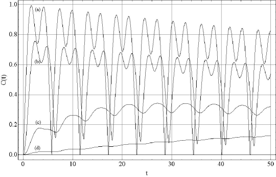
Figure 1: Dynamics of the concurrence $C(t)$ for the initial reduced density matrix $\hat{\rho}_{0}=|1,0\rangle\langle 1,0|$. The parameters of the model are chosen to be $\gamma_{1}=\gamma_{2}=0.001$, $\epsilon_{1}=2$, $\epsilon_{2}=1.1$, $K=1$, $T_{1}=0.2$, $T_{2}=0.5$ for different coefficients $\gamma_{0}$ in the memory kernel $k(t)$: curve $(a)$ corresponds to the Markovian case $k(t)=\delta(t)$; curves (b)-(d) post-Markovian cases; curve (b) $\gamma_{0}=1$; curve (c) $\gamma_{0}=0.1$; curve (d) $\gamma_{0}=0.01$.

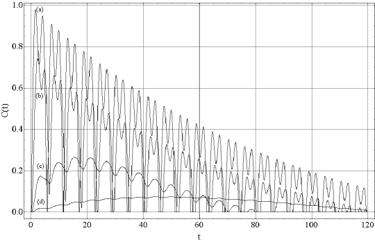
Figure 2: Dynamics of the concurrence $C(t)$ for the initial reduced density matrix $\hat{\rho}_{0}=|1,0\rangle\langle 1,0|$. The parameters of the model are chosen to be $\gamma_{1}=\gamma_{2}=0.001$, $\epsilon_{1}=2$, $\epsilon_{2}=1.1$, $K=1$, $T_{1}=1.2$, $T_{2}=1.5$ for different coefficients $\gamma_{0}$ in the memory kernel $k(t)$: curve $(a)$ corresponds to Markovian case $k(t)=\delta(t)$; curves (b)-(d) post-Markovian cases; curve (b) $\gamma_{0}=1$; curve (c) $\gamma_{0}=0.1$; curve (d) $\gamma_{0}=0.01$.

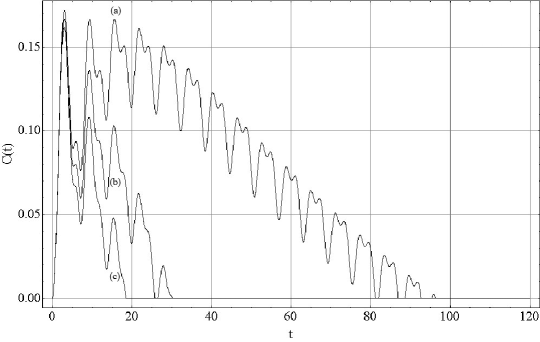
Figure 3: Dynamics of the concurrence $C(t)$ for the initial reduced density matrix $\hat{\rho}_{0}=|1,0\rangle\langle 1,0|$. The parameters of the model are chosen to be $\gamma_{1}=\gamma_{2}=0.001$, $\epsilon_{1}=1.5$, $\epsilon_{2}=1.1$, $K=1$, $\gamma_{0}=0.1$ for different temperatures of the ”baths”: curve $(a)$ corresponds to $T_{1}=0.2$, $T_{2}=0.5$; (b) $T_{1}=1.2$, $T_{2}=1.5$; (c) $T_{1}=2.2$, $T_{2}=2.5$.

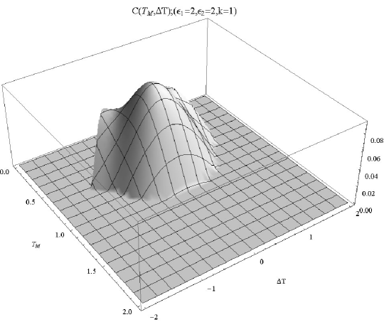
Figure 4: Steady-state concurrence $C(T_{M},\Delta T)$ as a function of the mean bath temperature $T_{M}=(T_{1}+T_{2})/2$ and temperature difference $\Delta T=T_{1}-T_{2}$ in the symmetric case $\epsilon_{1}=\epsilon_{2}=2$ with $K=1$.

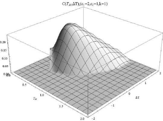
Figure 5: Steady-state concurrence $C(T_{M},\Delta T)$ as a function of the mean bath temperature $T_{M}=(T_{1}+T_{2})/2$ and the temperature difference $\Delta T=T_{1}-T_{2}$ in the case $\epsilon_{1}=2$, $\epsilon_{2}=1$, $K=1$.

V Results and Discussion

The dynamics of entanglement is analyzed in Figures 1-3. In Figures 1 and 2 the dynamics of the concurrence between the two qubits is shown for different coefficients $\gamma_{0}$ in the memory kernel $k(t)$ (for the Markovian case $\gamma_{0}=\infty$). One can see that with decreasing $\gamma_{0}$ memory effects play a more essential role in the system dynamics and practically suppress the oscillations in the concurrence dynamics due to the Hamiltonian dynamics of the system. In Figure 3 one can see that increasing the temperature of the baths destroys quantum correlations in the system. From Figure 3 and curve (c) on Figure 2 one can see the phenomenon of ”sudden death” of entanglement Refs. SDE1 ; SDE2 . The steady-state concurrence is analyzed in Figures 4 and 5. The detailed analysis of steady state concurrence for this model is given in Ref. qph . In Figures 4 and 5 we plot the steady-state concurrence for the symmetric $(\Delta\epsilon=0)$ and non-symmetric $(\Delta\epsilon\neq 0)$ cases as a function the mean temperature ($T_{M}=(T_{1}+T_{2})/2$) and the temperature difference ($\Delta T=T_{1}-T_{2}$) of the baths. One can see that in the symmetric case (Fig. 4) the maximal value of the entanglement corresponds to the thermodynamically equilibrium case $(T_{1}=T_{2})$ and in the non-symmetric case (Fig. 5) the maximum of the quantum correlations reaches in the thermodynamically non-equilibrium case.

In conclusion, we have found an analytical solution for a simple spin system coupled to bosonic baths at different temperatures in Markovian and Post-Markovian cases. We studied the influence of memory effect on the dynamics of entanglement.

References

• (1) Breuer, H.-P. The Theory of Open Quantum Systems / H.-P.Breuer, F.Petruccione. Oxford University Press, 2002. 648p.
• (2) Braun D., Creation of Entanglement by Interaction with a Common Heat Bath// Phys. Rev. Lett., 89, 2002, p277901.
• (3) Quantum States and Phases in Driven Open Quantum Systems with Cold Atoms/ S. Diehl et al., arXiv:0803.1482v1 [quant-ph].
• (4) Entanglement in many-body systems/ L. Amico et al., Rev. Mod. Phys. 80, 517 (2008).
• (5) Nonequilibrium thermal entanglement /L. Quiroga et al., Phys. Rev. A75, 032308 (2007).
• (6) Prosen, T. Third quantization: a general method to solve master equations for quadratic open Fermi systems/T. Prosen // New J. Phys. 10, 043026 (2008).
• (7) Mejia-Monasterio C., Heat transport in quantum spin chains: Stochastic baths vs. quantum trajectories/ C. Mejia-Monasterio, H. Wichterich// Eur. Phys. J. Spec. Top. 151, 113 (2007).
• (8) Burgarth D., Mediated homogenization/ D. Burgarth, V. Giovannetti // Phys. Rev. A 76, 062307 (2007).
• (9) Scala M., Dissipation and entanglement dynamics for two interacting qubits coupled to independent reservoirs/M. Scala, R. Migliore, A. Messina// arXiv:0806.4852v1 [quant-ph].
• (10) Sinaysky, I. Dynamics of nonequilibrium thermal entanglement/I. Sinaysky, F. Petruccione, D. Burgarth// Phys. Rev. A, 2008, 78, 062301.
• (11) Shabani, A. Completely positive post-Markovian master equation via a measurement approach / A. Shabani, D.A. Lidar// Phys. Rev. A, 2001, 71, 020101(R).
• (12) Goldman, M. Formal theory of spin–lattice relaxation/ M. Goldman// J.Magn.Reson., 2001, 149, 160-187.
• (13) Wootters, W.K. Entanglement of Formation of an Arbitrary State of Two Qubits / W.K. Wootters // Phys. Rev. Lett., 1998, 80, 2245-2248.
• (14) Non-Markovian dynamics of a qubit coupled to an Ising spin bath/ H. Krovi et al. // Phys. Rev. A 76, 052117 (2007).
• (15) Maniscalco, S. Non-Markovian dynamics of a qubit / S. Maniscalco, F. Petruccione// Phys. Rev. A, 2006, 73, 012111.
• (16) Al-Qasimi, A. Sudden death of entanglement at finite temperature / A. Al-Qasimi, D. F. V. James// Phys. Rev. A, 2008, 77, 012117.
• (17) Environment -Induced Sudden Death of Entanglement/ M. P. Almeida et al., Science. 316, 579 (2007).