SPT-09/050
A matrix model for plane partitions
B. Eynard 111 E-mail: bertrand.eynard@cea.fr
Institut de Physique Théorique de Saclay,
F-91191 Gif-sur-Yvette Cedex, France.
Abstract
We construct a matrix model equivalent (exactly, not asymptotically), to the random plane partition model, with almost arbitrary boundary conditions. Equivalently, it is also a random matrix model for a TASEP-like process with arbitrary boundary conditions. Using the known solution of matrix models, this method allows to find the large size asymptotic expansion of plane partitions, to ALL orders. It also allows to describe several universal regimes. On the algebraic geometry point of view, this gives the Gromov-Witten invariants of with branes, i.e. the topological vertex, in terms of the symplectic invariants of the mirror’s spectral curve.
1 Introduction
The statistical physics problem of counting plane partition configurations of some domain, as well as its various equivalent formulations, has become a very active and fascinating area of mathematical physics in the past years, culminating with Okounkov’s renowned work. Beyond a beautiful combinatorics problem, it has also many indirect applications, like a tiling problem similar to a discrete version of TASEP, i.e. the simplest model of out of equilibrium statistical physics, and algebraic geometry, as it plays a key role in the computation of Gromov-Witten invariants of some toric Calabi-Yau 3-folds, through the topological vertex method [3].
The works of Okounkov, Kenyon and Sheffield [48], have brought immense progress, in the understanding of large size asymptotics behaviors of plane partitions. It was observed, that in many universal regimes, the statistical properties of large plane partitions, is very similar to that of matrix models, and many works have taken advantage of that similarity.
Here, in this article, we show that there is not only a ”similarity” between plane partitions countings and matrix models, in fact we show that plane partitions IS a matrix model, even for finite size. As a consequence, we may use all the machinery developped for solving matrix models, and we are able to compute all orders corrections to the large size asymptotics.
Our matrix model, is a multimatrix model, with non-polynomial potentials. It may look very complicated at first sight, and its spectral curve may look rather complicated too. However, the solution of matrix models is expressed in terms of symplectic invariants, and up to a symplectic transformation (which does not change the symplectic invariants), our complicated matrix model’s spectral curve, is equivalent to the Harnack curve of Kenyon-Okounkov-Sheffield [48].
Moreover, our formulation allows to use the full toolbox of matrix models technology. For instance the method of orthogonal polynomials gives determinantal formulae for correlation functions, the integrable structure, Riemann-Hilbert problem, and much more. And the loop equations method allows to compute the large size expansion order by order [54, 53].
1.1 Main results of this article
Our main result is the theorem 3.1:
Theorem 3.1: The tiling model-plane partitions-tilings generating function, can be written as a matrix integral. (a more precise result is written in theorem 3.1). This identification is exact, it is not asymptotic.
An immediate consequence is obviously:
Corollary: All asymptotic limits of tiling model-plane partitions-tilings, are random matrix limit laws.
(but it remains to classify all possible random matrix limit laws).
Also, since our matrix model is a chain of matrices, classical results of matrix models apply:
Corollary: The matrix model is integrable, the generating function is a Tau-function, and for instance correlation functions are given by determinantal formulae of Janossi densities type [31].
We would like also to emphasize that our ”Tiling matrix model” identification works for very general cases, with almost any possible boundary conditions, we can also give weights to points of the domain to be tiled, some points can be forbidden (defects), or obliged, or just have an arbitrary weight.
The second part of our paper, starting at section 4, consists in ”solving” the matrix model. We do it explicitly only for some not too complicated boundary conditions. We recover the Harnack curves of Kenyon-Okounkov-Sheffield.
2 Some statistical physics models
2.1 Plane partitions
Consider 3 integers , and 3 partitions , for example:
| (2-1) |
A plane partition with boundaries , and of size , is a piling of cubic boxes in the corner of a room, with boundary conditions given by , for example:
![[Uncaptioned image]](/html/0905.0535/assets/x4.png) |
is the height of the plane-partition (height of the cubic boxes piling), (resp. ) is the extension towards left (resp. right), so that beyond (resp. ), the section is frozen to (resp. ).
The partition function we would like to compute is:
| (2-2) |
where is the number of boxes, i.e. the volume, it is called the ”weight” of .
This partition function is the so-called ”topological vertex” in topological string theories [3], it is the building block to compute Gromov-Witten invariants of all toric Calabi-Yau 3-folds [7, 14, 3, 52, 56, 57, 61, 62, 67, 55].
From the combinatorics point of view, it is the generating function for counting plane partitions with given boundaries and weighted by their volume. From the statistical physics point of view, it can be viewed as a model for a growing 3-dimensional crystal in the corner of a room. All those topics have remained important research areas in physics and mathematics, and it would be difficult to summarize all what has been done. Let us mention that Kasteleyn [44, 45] found an explicit expression for the partition function of a domino-tiling, which can be rephrased as plane partition, and since then, the subject has been studied a lot, see for example [16, 47, 23].
2.1.1 Remark: semi-standard tableaux
If we slice our plane partition at all integer times (time = horizontal coordinate) , at each time the slice is a 2-dimensional partition .
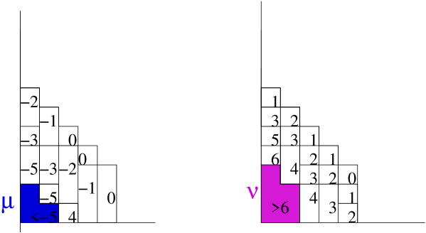 Figure 1: A plane partition is equivalent to the data of two semi-standard Young tableaux of the same shape . Each of these two tableaux, is the superposition of growing (or decreasing) partitions .
It is then clear that partitions are growing from to , and then decreasing from to :
| (2-3) |
where is the partial ordering of partitions ( means that can be obtained from by removing boxes). Since we have , we may draw all with inside the Ferrer diagram of , and we write in each box, the time at which the box appears for the first time. We do the same for , and we have two semi-standard tableaux with the same shape . A semi-standard tableau is a Ferrer diagram with integer entries decreasing along columns, and strictly decreasing along rows. See fig.1.
When , and , the statistics of the partition is the sum over all pairs of semi-standard tableaux of shape , i.e. it is the Plancherel measure [64, 65, 69]:
| (2-4) |
We shall study this limit in section 7.4.
2.2 Jumping non-intersecting particles
T.A.S.E.P. means ”totally asymmetric exclusion process” [51], it is the simplest model of statistical physics out of equilibrium, it has focused considerable amounts of works [18, 19, 63, 35, 36, 38], and it is still intensively studied. It is a model of self avoiding particles which can either stay at their place, or jump 1 step forward, provided that the next space is unoccupied. In the dynamics we shall be considering here, time is discrete, and at each unit of time, several particles can jump.
It is well known that plane partitions can be rephrased in terms of self-avoiding jumping particles model which is a kind of discrete T.A.S.E.P. [64, 65, 69, 68, 43, 6, 5, 2], let us re-explain it here.
Let us draw in red the non-intersecting lines going through tiles
![]() and
and ![]() :
:
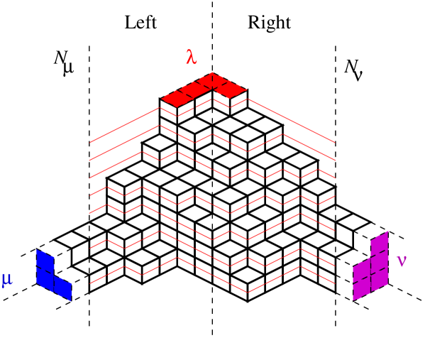 Figure 2:
The level lines, go only through upright or downright tiles, they form non-intersecting lines whose slopes are piecewise .
Figure 2:
The level lines, go only through upright or downright tiles, they form non-intersecting lines whose slopes are piecewise .
The tiles ![]() correspond to upright lines with slope ,
and the tiles
correspond to upright lines with slope ,
and the tiles ![]() correspond to downright lines with slope .
The intersection of those red lines with integer time lines are interpreted as positions of some particles ( is at the top). See figure 2.
correspond to downright lines with slope .
The intersection of those red lines with integer time lines are interpreted as positions of some particles ( is at the top). See figure 2.
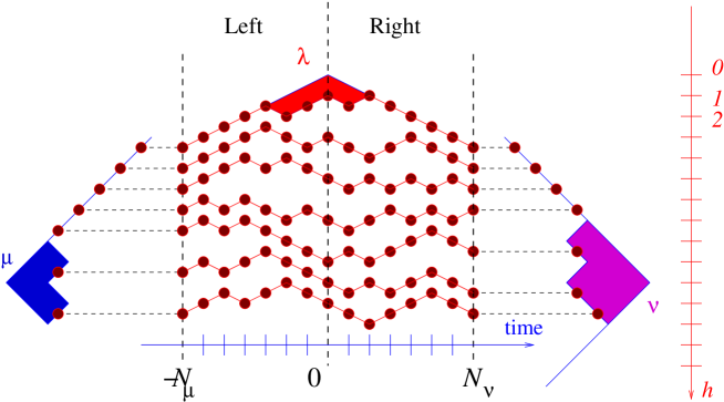 Figure 3:
Therefore, a plane partition , can also be described as the data of sets of variables:
| (2-5) |
such that for every integer , the are non-negative ordered integers:
| (2-6) |
where is the profile function of the partition .
At time and time we have:
| (2-7) |
and at each time , we have a partition :
| (2-8) |
we thus have and .
Moreover we have:
| (2-9) |
This is what we call here a discrete T.A.S.E.P. process:
there are particles at positons , and at each unit of time, they jump by , and they can never occupy the same position (in the usual formulation of TASEP, particles jump by 0 or 1, and here we have tilted the picture so that they jump by , which is clearly the same thing up to ).
2.2.1 Summary plane partition and jumping particles
A plane partition with boundaries , and of size , is equivalent to , , , such that:
| (2-10) | |||||
| (2-11) | |||||
| (2-12) | |||||
| (2-13) |
The total numer of boxes in the partition is:
| (2-14) |
2.2.2 Height function and density
There is a relationship between the height function of the pile of cubes, and the density of ’s. Define the density at time as the Dirac-comb distribution:
| (2-15) |
The profile of the partition at time is recovered from the integral of as follows. Define the integrated density:
| (2-16) |
computes the index such that . Then, define the function
| (2-17) |
The plot of against is the shape of the partition is at time . See fig.4.
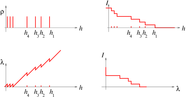 Figure 4: The density encodes the profile of the partition .
The surface of the pile of cubes in is recovered from plotting the partition at all times, i.e. it is given by:
| (2-18) |
2.3 Lozenge tilings
Another representation of plane partitions and the self-avoiding particle model, is with lozenge tilings of the rhombus lattice.
The rhombus lattice is a tiling of the plane, with lozenges ![]() , whose centers are at the positions such that and , see fig 5.
, whose centers are at the positions such that and , see fig 5.
 Figure 5: The rhombus lattice is a tiling of the plane, with lozenges whose centers are at the positions such that and . Notice that we orient from top to bottom.
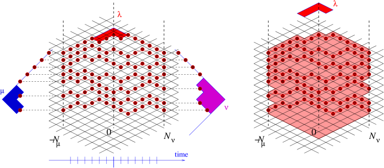 Figure 6:
A plane partition configuration, can be represented as self-avoiding walks in some domain of the rhombus tiling of the plane. The white lozenges are forbidden, they are related to the 3 boundary partitions .
Figure 6:
A plane partition configuration, can be represented as self-avoiding walks in some domain of the rhombus tiling of the plane. The white lozenges are forbidden, they are related to the 3 boundary partitions .
A plane partition or a self-avoiding particle model configuration can be represented as oriented self-avoiding walks in some domain of the rhombus tiling of the plane. See figure 6. At a given time, each walker moves to the right , and either up or down .
The centers of occupied lozenges are at positions , .
The domain is the domain which contains all possible paths. is a subdomain of the hexagon defined by the following 6 inequalities:
| (2-19) | |||||
| (2-20) | |||||
| (2-21) |
Indeed, since at each time, and particularly at and , we have , no path starting at some at and ending at some at can go out of this hexagon.
Moreover, the domain can be chosen such that some positions are forbidden, in fact we allow to be any arbitrary subset of the maximal hexagon.
For example for plane partitions, the positions corresponding to the boundaries are forbidden, i.e. has holes corresponding to the 3 partitions at the boundaries:
At , we remove from , all lozenges which are not of the form for some .
At , we remove from , all lozenges which are not of the form for some .
At every time we impose .
See fig 6.
2.3.1 Defects
It is interresting to generalize our model to include walks on more general domains, not only limitted by 3 boundary partitions. In particular, we may allow defects and holes at almost any place.
Consider a connected compact domain in the rhombus lattice, but not necessarily simply connected.
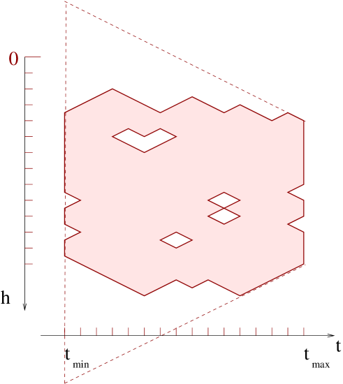 Figure 7: The maximal domain of is the region comprised in the dashed line.
Definitions:
The maximal domain of is the intersection of with (see the dashed region in figure 7 and figure 8).
The defect of , is . The shadow of , is the domain which is unaccessible to particles moving in , with slopes . We have .
Those notions are illustrated in fig 8.
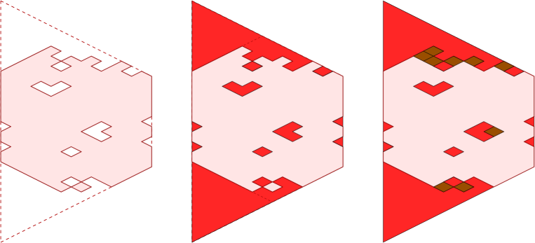 Figure 8: Consider a given domain . Its maximal domain is represented with dashed line on the left figure (it is obtained by lines of slopes starting from the extremities of the domain at ).
In the middle figure we have represented the defect of , that is (the red region).
In the right figure we have represented the shadow of , that is the domain which is unaccessible to particles moving in , with slopes (the brown+red region), it contains . This means that particles moving in can never enter the brown tiles.
Figure 8: Consider a given domain . Its maximal domain is represented with dashed line on the left figure (it is obtained by lines of slopes starting from the extremities of the domain at ).
In the middle figure we have represented the defect of , that is (the red region).
In the right figure we have represented the shadow of , that is the domain which is unaccessible to particles moving in , with slopes (the brown+red region), it contains . This means that particles moving in can never enter the brown tiles.
Definition:
The minimal defect of , is the smallest subdomain of , such that:
| (2-23) |
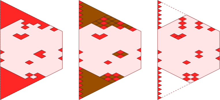 Figure 9:
The left figure represents the domain and its defect in red.
The right figure represents (in red) the minimal defect of .
The middle figure shows that both and have the same shadow (in brown+red).
Figure 9:
The left figure represents the domain and its defect in red.
The right figure represents (in red) the minimal defect of .
The middle figure shows that both and have the same shadow (in brown+red).
2.3.2 Domain at time t
Let us call , the slice of the domain at time , i.e. the set of allowed positions of particles at time :
| (2-24) |
Let us call the slice of at time , i.e. the position of holes:
| (2-25) |
Let us assume that the number of particles , is such that:
| (2-26) |
in other words such that it is indeed possible for avoiding particles to move in .
Remark 2.1
Most often we will choose , i.e. the position of all particles at time are fixed. Very often we will also choose the domain such that , i.e. the position of all particles are also fixed at time .
But we emphasize that the method we present here works also without those assumptions.
2.3.3 Filling fractions
In general, the domain at time , is a union of intervals:
| (2-27) |
If the intervals are disconnected, no particle can jump from one interval to another, and thus the number of particles moving in an interval is constant in time, until intervals join. We may thus fix the number of particles in each interval. Call it filling fraction of the interval at time . We have:
| (2-28) |
In general, if the domain has holes, there are independent filling fractions.
2.4 Partition function
The partition function which we wish to compute is:
| (2-29) |
where at each time we have , and where and have fixed values given by two partitions and (encoded by the boundaries of ):
| (2-30) |
We count the configuration with a weight , and with weights per number of upward jumps ![]() between time and , and with weights per number of downward jumps
between time and , and with weights per number of downward jumps ![]() between time and .
between time and .
It can be rewritten:
| (2-33) | |||||
where here, is the Kroenecker’s -function.
2.5 Applications
In topological string theory, Gromov Witten invariants of toric Calabi-Yau 3-folds are computed with the topological vertex, which is the following sum of plane partitions [3, 58]:
| (2-35) |
When , and , and , this sum is known, it is the Mac-Mahon formula:
| (2-36) |
The Razumov-Stroganov conjecture [4, 22] has put forward a problem of combinatorics of totally symmetric sel-complementary plane partitions (TSSCPP), and the claim is about the relationship with the combinatorics of alternating sign matrices (ASM). There is a 6-vertex matrix model formulation for ASM [72], and it would be interesting to also have a matrix model for TSSCPP, that’s what we address in section 8 below.
3 Matrix model
We are going to represent our self avoiding particle process partition function eq. (2-29) as a multi-matrix integral.
Let us sketch the idea of the next subsection: we shall introduce normal matrices of size , for all integer times between and , whose eigenvalues are the . Moreover, we shall Fourrier-transform the functions which enforce :
| (3-1) | |||||
| (3-2) | |||||
| (3-3) |
i.e. we shall introduce some Lagrange multipliers at all half-integer times, and we will introduce a hermitian matrix whose eigenvalues are the Lagrange multipliers , , which implement the functions for the jumps between time and . See fig.10.
More generally, if we wanted to allow jumps of several steps , we would take the Fourrier transform of .
The non-intersecting condition for paths can be realized as a determinant, like Gessel-Viennot formula [37], which allows to rewrite
| (3-5) |
and we recognize that this expression is the Itzykson-Zuber-Harish-Chandra formula [39, 41]:
| (3-6) |
This is the key to obtain a matrix integral, it introduces angular degrees of freedom in addition to eigenvalues:
| (3-7) |
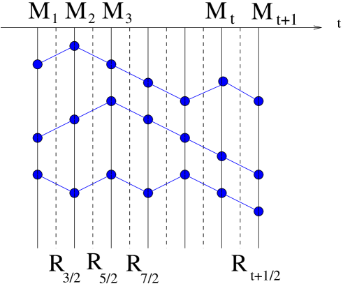 Figure 10: We introduce a chain of matrices. The eigenvalues of the random matrices with integer, are the random . And the with half integer are Lagrange multipliers which enforce the relations .
And we shall introduce some potential for the matrices , to ensure that their eigenvalues are in , and and enforce the initial values at time or .
We shall find that the sum over ’s can be rewritten as a ”chain of matrices” matrix model.
So, let us describe the model now.
3.1 The multi-matrix model
Let us consider the following multi-matrix integral:
| (3-9) | |||||
Each integral over with is over the set of hermitian matrices of size , and each integral over with is over the set of anti-hermitian matrices of size . And there is no integration over , which is a fixed external field, which we choose equal to:
| (3-11) |
The potentials or are defined as follows:
for half-integer:
| (3-12) |
this potential for is the Fourrier transform of the jumps, see eq. (3-1), we have just rescaled by .
and for integer, , we choose the potential such that:
| (3-13) |
can be more or less interpreted as the characteristic function of the domain , or more precisely, the complementary domain of the defect .
However, this definition does not define a unique potential , and many potentials may have the property eq. (3-13). In particular, we see that the value of in the shadow of , more precisely in , is undetermined. We show below some rather canonical examples of satisfying those constraints.
We will see below that the value of the partition function does not depend on the choice of .
and for , we choose the potential such that:
| (3-14) |
In other words, we do not even require that in the domain, we only require that it is .
Examples of :
Since our domain is compact, we have to find a potential with prescribed values at a finite number of points, and a possibility is to choose to be the Lagrange interpolating polynomial going through the prescribed values.
For example, if our domain at time is contained in the interval
| (3-15) |
we may choose the potential as the Lagrange interpolating polynomial:
| (3-16) |
Another possibility is to take the limit :
| (3-17) |
or we may also choose:
| (3-18) |
Depending on the type of applications we are interested with, it is sometimes more convenient to work with a potential of type eq. (3-16) or a potential of type eq. (3-17), or also their -deformations, or sometimes other potentials having property eq. (3-13).
In general, we see that must have logarithmic singularities on , and thus we may write:
| (3-19) |
where can be any arbitrary entire function which vanishes on , and where is an analytical function such that if we have . Since fixing the values of and does not fix the values of and at those points, we see that what characterizes is that it has simple poles with residue in , plus an almost arbitrary analytical function.
3.1.1 Diagonalization
Let us diagonalize all matrices in eq. (3-9). One needs to know that any normal matrix (and in particular hermitian matrices) can be diagonalized by a unitary transformation:
| (3-20) |
and the matrix measures are:
| (3-21) |
where is the Haar measure on and is the Vandermonde determinant:
| (3-22) |
Similarly for the matrices :
| (3-23) |
3.2 Relation between the matrix model and the self-avoiding particles model
3.2.1 Integrals over Lagrange multipliers
Then let us perform the integral over , we have:
| (3-36) | |||||
| (3-37) | |||||
| (3-39) | |||||
| (3-41) | |||||
This term implies that there must exist some permutation such that
| (3-43) |
with respective probabilities . And in particular, since this is true for , we have :
| (3-44) |
In particular that implies that , and thus if and if . In particular, the matrix integral is indeed independent of the choice of , provided that it satisfies eq. (3-13).
Then, since the quantities we are summing are symmetric, we can assume, up to a multiplication by , that all are ordered:
| (3-45) |
and this yields a factor , which we shall discard because we consider the partition function up to global trivial constants.
In other words, the result of the integral is a sum over , where are ordered integers:
| (3-47) | |||||
where the sum over , is such that:
| (3-49) |
and
| (3-50) |
Then, notice that if and if . In other words, the sum is only over ’s such that
| (3-51) |
In other words, we have a self-avoiding particle process on the rhombus lattice, which avoids a prescribed domain , i.e. we recover our self-avoiding particles partition function:
Theorem 3.1
The self-avoiding particles model partition function in a domain , is proportional to the matrix integral :
| (3-52) |
where the constant depends only on and , and nothing else. It contains the normalization factors, such as the volumes of unitary groups, and the powers of .
This theorem implies immediately, as a tautology, that whatever limit we consider (for instance large size limit, limit, bulk regime, behavior near edges, ), the asymptotic statistical properties are always matrix models limit laws !
This explains why one finds sine kernel laws in the bulk, Tracy-Widom laws near some boundaries, Pearcey laws, and many more…
3.3 Determinantal formulae
Theorem 3.1 allows to apply to the self-avoiding particles model and plane partitions, all the technology developed for matrix models, in particular the methods of orthogonal polynomials [53, 54].
Consider a ”chain of matrices” integral:
| (3-53) |
where are some potentials, where is the set of normal matrices having their eigenvalues on contour , and where is not integrated upon.
The Eynard-Mehta theorem [31] shows that correlation functions of densisities of eigenvalues , are determinants. Namely, there exist some kernels such that:
| (3-54) |
where the kernels are Christoffel-Darboux kernels for some families of biorthogonal polynomials.
4 Matrix model’s topological expansion
The good thing about theorem 3.1, is that the general expansion of matrix integrals of the chain of matrices type is known to all orders.
4.1 Generalities about the expansion of matrix integrals
See appendix C for a more detailed description.
Consider a ”chain of matrices” integral:
| (4-1) |
where are some potentials, where is the set of normal matrices having their eigenvalues on contour , and where is not integrated upon.
In some good cases (depending on the choice of potentials and paths ), such an integral has a large expansion of the form:
| (4-2) |
Such an expansion does not always exist. It exists only if the paths which support the eigenvalues, are ”steepest descent paths” for the potentials (see e.g. [28, 25]). Finding the steepest descent paths associated to given potentials is an extremely difficult problem.
Fortunately, many applications of random matrices regard combinatorics, i.e. they are formal series in some formal parameter, and very often, the corresponding so-called “formal matrix integrals” do have a large expansion almost by definition222For formal matrix integrals, the integration paths for eigenvalues, are most often not known explicitely, they can be determined so that a large power series expansion does exist., and eq. (4-2) holds order by order in the formal parameter (a formal parameter which is not necessarily ). Here, we are considering applications to statistical physics, our partition functions are formal series, and we shall assume that such an expansion exists (order by order in a suitable formal parameter).
The problem is then to compute the coefficients .
The answer was found in [33], by using loop equations (i.e. Schwinger-Dyson equations in the context of matrix models), and which just correspond to integrations by parts.
The solution proceeds in two steps (which we explain below):
1) Compute the ”spectral curve” of the matrix model. The spectral curve is a pair of two analytical functions of a variable living on a Riemann surface. The spectral curve is obtained from the ”classical limit” of the integrable system whose tau-function is the matrix integral. Roughly speaking, if we eliminate , the function is more or less the equilibrium density of eigenvalues of the first matrix of the chain. We explain in appendix C how to find the spectral curve of a general chain of matrices. We emphasize that associating a spectral curve to a given matrix model, is something already done in the matrix models literature.
4.2 Spectral curve of the self-avoiding particles matrix model
We recall in appendix C the main results of [33], i.e. how to compute the spectral curve of an arbitrary chain of matrices. Here, in this section, we merely apply the general recipe of [33] (see appendix C) to our matrix integral eq. (3-9), and we give a ”ready to use recipe”.
Recipe for finding the spectral curve of the matrix integral eq. (3-9):
Find analytical functions of a variable ( belongs to a Riemann surface ). There is one such analytical function for each matrix of the chain, plus one additional function at the end of the chain. Let us call them:
| (4-4) |
Those functions are completely determined by the following constraints:
-
1.
Those functions must obey the following system of equations :
(4-5) -
2.
There exists a point in , which we call , such that has a simple pole at , and we have:
(4-6) -
3.
There exists points , such that is an eigenvalue of :
(4-7) and has simple poles at the points and behaves like:
(4-8) -
4.
Define for :
(4-9) and call it ”the resolvent” of the matrix . We require that , is analytical in a vicinity of , and behaves like:
(4-10) and can be analytically continued to
(4-11) where we recall that is a compact region of .
-
5.
Typically, may have branchcuts or isolated singularities, like poles or log singularities. The set of points at which is not analytical is called the support:
(4-12) The interior of is called ”the liquid region” (it contains the cuts, it excludes the isolated singularities). We have , and
(4-13) If , we require that : is connected.
-
6.
If the domain at time is a disconnected union , we require that :
(4-14) where the integration contour surrounds the interval in the plane, in the clockwise direction.
Finding functions satisfying all those requirements for a general domain, with general weights is a difficult problem. But for not too complicated domains and weights, some simplifications may occur, and we will see many examples of explicit solutions below.
From now on, let us assume that we have found the functions and satisfying all the requirements. Once we have found a solution to this problem, i.e. found the functions and , we define the spectral curves:
Definition 4.1
The spectral curve at time is the pair of functions:
| (4-15) |
Remark 4.1
Because of eq. (4-5), the following 2-forms in , restricted to the spectral curve, are equal:
| (4-16) | |||||
| (4-17) |
and therefore, the spectral curves and are symplecticaly equivalent:
| (4-19) |
4.3 Symplectic invariants and topological expansion
The symplectic invariants were introduced in [27]. To any spectral curve , one can associate, by simple algebraic computations, an infinite sequence of complex numbers , . We recall their definition in appendix B.
One of their main properties, is that if two spectral curves and are symplectically equivalent, then we have .
In our case, because of eq. (4-19), we have:
| (4-20) |
and therefore is independent of , the ’s are conserved quantities.
It was proved in [33], for any chain of matrices, and here we apply it to our case, that:
Theorem 4.1
| (4-21) |
where the right hand side is independent of .
This theorem holds order by order in some appropriate formal large parameter expansion. We will see examples below, where the formal parameter can be the size of the system, or , or ,…etc.
4.3.1 Arctic circle
For most interesting applications, there is some ”large parameter ” in our problem (typically the size of the domain , or , or sometimes other parameters), such that the spectral curve scales like , typically:
| (4-22) |
(where we write for a spectral curve ).
The large spectral curve was already computed in many works and in particular by Kenyon-Okounkov-Sheffield [48] who found the limit shape of the liquid region.
From the homogeneity property of ’s (see [27] and appendix B) we have , i.e. we find a large expansion:
| (4-23) |
Such an expansion is not very useful if depends on .
In fact, in many examples related to TASEP and plane partitions, we find that the spectral curve depends on , but up to a symplectic transformation we have miraculously (this happens for instance in the matrix model considered in [26]):
| (4-24) |
which implies:
| (4-25) |
and in that case, is independent of .
This miracle is deeply related to the structure of the self-avoiding particles model partition function, and with the so called ”arctic circle phenomenon”, i.e. the fact that the system freezes beyond a certain size [42]. This can also be related to the fact that we have some arbitrariness in choosing the potentials , and we could choose some potentials which depend on in an appropriate way such that the spectral curve would not depend on . Although it is doable in theory, finding the corresponding ’s seems horrendous. A rather explicit example of this phenomenon was discussed in [26].
Only in the case where we have this ”arctic circle phenomenon”, we have:
| (4-26) |
where the spectral curve is the curve derived from the Harnack curve of Kenyon-Okounkov-Sheffield [48].
In that case, we can compute the large expansion of our self-avoiding particles model model, to all orders in , not only the large leading order limit.
4.4 Reduced matrix model
For a fully general domain , there are as many equations eq. (4-5) to solve as the size of the domain, but, when the domain has very few defects, many of those equations simplify considerably, and we may consider a reduced problem.
Notice, that everytime , we may choose for all , and thus . Therefore, it is possible to simplify dramatically the equations determining the spectral curve.
Notice also, that there can be many times at which , but since particles can only follow lines with slopes , many places (the shadow of ) are never visited. In other words, we may replace the defects by the minimal defect of , and since in general is a very small subset of , this allows to simplify the problem.
Only the minimal defect needs to be specified.
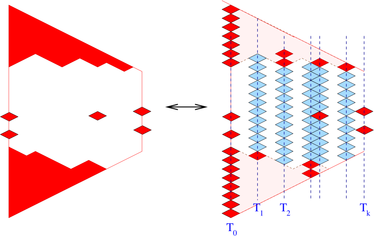 Figure 11:
The left figure represents the domain and its defect in red.
The right figure represents the minimal defect in red. If there are times containing red lozenges, then the reduced matrix model is a matrix model.
The potentials of the reduced model must be such that at the center of red lozenges, and at the blue ones. The values of elsewhere are arbitrary.
Figure 11:
The left figure represents the domain and its defect in red.
The right figure represents the minimal defect in red. If there are times containing red lozenges, then the reduced matrix model is a matrix model.
The potentials of the reduced model must be such that at the center of red lozenges, and at the blue ones. The values of elsewhere are arbitrary.
Let the times at which be called:
| (4-27) |
among those ’s we include the extremities and :
| (4-28) |
The spectral curve equations eq. (4-5) can be rewritten:
| (4-29) |
We thus define:
| (4-30) |
and the potentials
| (4-31) |
i.e.
| (4-32) |
The loop equations eq. (4-29) are equivalent to:
| (4-33) |
One recognizes that these equations are exactly the equations of the spectral curve of another matrix model, which is a chain of matrices, but with only matrices instead of , and we get the following result:
Theorem 4.2
The matrix model partition function can be rewritten:
| (4-35) | |||||
i.e. a chain of matrices, instead of a chain of as we had before.
Notice that knowing , we can reconstruct for all times :
| (4-37) |
and if
| (4-38) |
5 Liquid region
Our spectral curve is thus given by a collection of functions and , defined for all integer times . We assume that the potentials are non-zero only for times , and the domain at time is the union of intervals:
| (5-1) |
with filling fractions , i.e. we require that there are particles in .
This implies that the potentials are of the form:
| (5-2) |
where is some analytical function, and is the digamma function. We used the well known property of that:
| (5-3) |
5.1 Interpolation to real times
It is in fact better to enlarge these definitions to all times (not necessarily integers or half-integers) by interpolation:
| (5-4) |
and we write:
| (5-5) |
i.e.:
| (5-6) |
The function is discontinuous at time :
| (5-7) |
Similarly we define for :
| (5-8) |
If is constant over some interval, then we can find explicitly the interpolating function:
| (5-9) |
where is defined as (see appendix A):
| (5-10) |
If , we have:
| (5-11) |
Notice that this expression depends linearly on .
5.2 Densities of particles
Consider the density of particles at time (in section 2.2.2, we have seen that these densities are related to the profile of the plane partitions):
| (5-12) |
We also consider their Stieltjes transforms, i.e. the resolvents:
| (5-13) |
Let us assume that our model has a formal large expansion in some parameter , it follows from the general solution of the chain of matrices [33], that one can write:
| (5-14) |
where the first term is given by eq. (4-9):
| (5-15) |
and the density is the discontinuity of across :
| (5-16) |
All the higher corrections for were also computed in [33], and they are the correlators of the symplectic invariants (see appendix B or [27]) of the spectral curve . In other words, if we know the spectral curve at time , there is a simple recursive algebraic algorithm to compute all the corrections, of any correlation function, to all orders in . We shall not detail this here.
Remark 5.1
Let us mention, that if the arctic circle property does not hold (this may be the case for complicated domains), then the spectral curve may depend on , and thus all the depend on . In other words, eq. (5-14) is true as an equality of formal series, but it is not really a large expansion. In particular, is not necessarily the large limit. When the arctic circle property holds, then, the are independent of , and we really have a large expansion. We will see examples where this holds, below in section 7.
Let us now study the leading term.
can have various sorts of singularities, it can have isolated singularities, like poles, or log singularities, and it can have branchcuts. In terms of the density , the poles of correspond to -Dirac distributions, and cuts correspond to smooth positive densities. Log singularities of correspond to discontinuous jumps of the density.
Notice that eq. (4-10) implies that is normalized, with total weight :
| (5-17) |
but if we exclude the isolated singularities, i.e. if we integrate only in the liquid region (the interior of the support), we have:
| (5-18) |
Notice also that if is disconnected, i.e. a union of intervals , we have required that the filling fraction is fixed:
| (5-19) |
5.3 The Envelope of the liquid region
The liquid region, is the interior of the support of the density, i.e. it excludes all the isolated singularities of , it contains only the cuts.
The complement of the liquid region in , is called the ”solid” region, it contains the isolated singularities of , and possibly their accumulation points.
The boundary of the liquid region is called the envelope of the liquid region. It is given by the branchpoints.
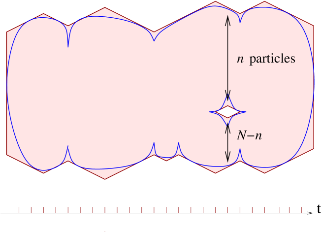 Figure 12: Given a domain , we compute its spectral curve for all times . From the spectral curves we compute the densities , whose supports are contained in . The interior of the support is called the ”liquid region”.
The liquid region is delimited by the envelope, which is a curve contained in .
The points on the envelope are branchpoints of the functions , i.e. zeroes of
We shall see below that the envelope has some special properties of tangency to the domain .
Figure 12: Given a domain , we compute its spectral curve for all times . From the spectral curves we compute the densities , whose supports are contained in . The interior of the support is called the ”liquid region”.
The liquid region is delimited by the envelope, which is a curve contained in .
The points on the envelope are branchpoints of the functions , i.e. zeroes of
We shall see below that the envelope has some special properties of tangency to the domain .
The branchpoints at time , are zeroes of the differential form , i.e. they are the points where the density has a vertical tangent:
| (5-20) |
where is the differential with respect to . Not all branchpoints are boundaries of the liquid region, let us consider only those which are on the envelope. The boundary of the liquid region is thus at such that:
| (5-21) |
By definition, the envelope is a curve contained in . Let us study some of its properties.
5.3.1 Tangency
Theorem 5.1
If a point of the envelope has a tangent of slope , then this point must be on the boundary of the shadow of .
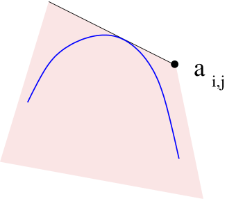 Figure 13:
A point of the envelope at which the tangent has a slope , is necessarily on the boundary of the shadow of , this means that there is a point of the defect on the tangent.
Figure 13:
A point of the envelope at which the tangent has a slope , is necessarily on the boundary of the shadow of , this means that there is a point of the defect on the tangent.
proof:
Let be such that the point is a point of the envelope at which the tangent has slope (resp. ). Let , i.e. we have .
Since on the envelope we have , we see that at all times we have:
| (5-22) |
and therefore we must have:
| (5-23) |
and, from eq. (5-8), this implies that
| (5-24) |
Then, if (resp. ), we see from eq. (5-8), that :
| (5-25) |
and in particular at , we have:
| (5-26) |
which means that the tangent to the envelope at point , passes through the point at time :
| (5-27) |
Then, notice that can be equal to or , only if has a singularity at . Because of eq. (4-33), we see that, singularities of can occur only if has a singularity.
Remember that has no singularity on , it has singularities only at the defects , and thus, this means that the point belongs to the defect . But we know that the point belongs to , and the slope between the points and is equal to , i.e. the point is in the shadow of the defect .
5.3.2 Local Convexity
In the classical case, where is constant, we have a convexity property:
Theorem 5.2
If is constant in time, the liquid region is locally convex.
proof:
The density at time must have a real support, starting at a branchpoint, i.e. at . Consider that, up to a reparametrization of , and up to trivial translations in and , we can write localy, near the branchpoint point we write:
| (5-28) |
and up to a rescaling of , we assume . Notice from eq. (5-11), that the assumption constant guarantees that is linear in , there is no term.
The branchpoint at time is at given by , i.e.:
| (5-29) |
i.e., the envelope is, up to order :
| (5-30) |
Our assumption on the reality of the supports, implies that for all , and therefore and must be real quantities.
The point such that is:
| (5-31) |
The function is then given by solving eq. (5-8):
| (5-32) | |||||
| (5-33) |
and therefore
| (5-34) |
and the density , with is, up to order :
| (5-35) |
This implies that in the liquid region. If the liquid region is above , we must have , and if the liquid region is below , we must have . In all cases, the liquid region is locally convex.
Remark 5.2
If we are not in the classical case, i.e. if is not constant, then is not linear in , there maybe a second derivative , and the envelope is locally:
| (5-36) |
and although has a constant sign, can have any sign, and the envelope is not necessarily convex.
5.3.3 Cusps
Notice that is discontinuous at , i.e. there is a left value and a right value. This implies that has a right tangent and left tangent, and thus generically, the envelope has cusps at .
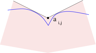 Figure 14: The envelope has a cusp at .
5.3.4 Genus and holes
Condition 6 of section 4.2, i.e. eq. (4-14) tells us that the spectral curve must have at least as many non trivial cycles as the number of holes in our domain, i.e. the genus of our spectral curve is at least the number of holes, and generically, it coincides with the number of holes.
In particular, if we consider a simply connected domain with no holes, we can expect to have genus , which means that the functions and are analytical functions of a complex variable . The Riemann surface in which lives can be chosen as a domain of the complex plane.
6 Asymptotic regimes
Of course, our model depends on so many parameters (shape of the domain, coefficients , potentials , …) that it is almost impossible to classify all possible asymptotic regimes. However, a few asymptotic regimes are more relevant for applications in statistical physics or algebraic geometry.
We classify them into 2 kinds:
macroscopic asymptotic regimes, which describe the behavior of the partition function, i.e. the statistics of our self-avoiding particles model at the scale of the size of the domain. Typically, we shall consider asymptotic behaviors for large size, of for small .
microscopic asymptotic regimes, which describe the statistics of our self-avoiding particles model particles in a very small region of the domain, typically, the behavior in the bulk, or near the edges, especially near special points, like near the envelope, or near cusps of the envelope.
Let us comment a few of them, and let us emphasize that our method, works for all possible asymptotic regimes, and it gives not only the leading order asymptotics, it gives the full asymptotic expansion to all orders.
6.1 Classical case q=1, and large size asymptotics
Classical means that we choose . Here, we shall assume that the weights are constant, although the general case is doable by the same methods.
Consider a domain whose size is . Assume that there are defects, and does not depend on :
| (6-1) |
The defects are at times , where are independent of , and the defect at time is the union of intervals:
| (6-2) |
where again and don’t depend on .
Assume also that the number of particles scales like :
| (6-3) |
and the number of particles in each interval scales like :
| (6-4) |
and of course
| (6-5) |
See fig 15.
 Figure 15: A polygonal domain with defect at times .
The envelope of the spectral curve, is the algebraic curve of smallest degree, tangent to all boundaries.
Figure 15: A polygonal domain with defect at times .
The envelope of the spectral curve, is the algebraic curve of smallest degree, tangent to all boundaries.
6.1.1 The spectral curve
The spectral curve equations eq. (4-33) are:
| (6-6) |
where we choose the potentials according to eq. (3-19):
| (6-7) |
where has no singularity, and is the digamma function. We used the well known property of that:
| (6-8) |
Moreover, the last matrix of the chain is not integrated upon. Its spectrum is , i.e. it is delimited by the intervals . Then, equation eq. (4-8) reads:
| (6-9) |
6.1.2 Rescaling
Since our model is defined as a formal power series, and we are looking for the large expansion, we should try to find the spectral curve in the large expansion. In that purpose we rescale the variables:
| (6-10) |
and we use Stirling’s asymptotic formula for the and functions, see appendix A:
| (6-11) |
where are the Bernouilli numbers.
That gives:
| (6-12) |
where the term is, to each power of , a rational function of with poles at or , plus possibly an arbitrary analytical function with no singularity. We also have:
| (6-13) |
where the term is, to each power of , a rational function of with poles at or , plus possibly an arbitrary analytical function with no singularity.
6.1.3 Singularities
We see from eq. (6-12),and eq. (6-13), that if , the ratio has a zero, and thus either has a zero, or has a pole, or both.
In fact, since and are multivalued function of , there might be several points on the spectral curve such that . In that case, it may happen that corresponds to in one sheet, and corresponds to in another sheet. Or if both has a zero, and has a pole at the same point, this means that has a double zero, i.e. has a zero, and this means that we are at a branchpoint, i.e. the point where two sheets meet.
Therefore, we shall assume that generically both possibilities occur, and we conclude that:
has a zero when or , and has a pole when or .
Since the ’s and ’s have only meromorphic singularities, it is natural to look for an algebraic solution, i.e. such that and are meromorphic functions on an algebraic curve . Indeed, our freedom to choose the potential can be used to eliminate all the singularities except those described above.
The problem then consists in finding algebraic functions , , such that:
,
has a simple zero when or , and has a simple pole when or .
the density measures (where are the two points on each side of the support) must have their supports in (in particular the supports are real). Those reality conditions for an algebraic curve, are closely related to the conditions which defines the Harnack curve in Kenyon-Okounkov-Sheffield [48].
6.1.4 The large size limit: Harnack curve
So, we have to find a spectral curve, and its envelope, satisfying many equations (which give the poles and zeroes), as well as many reality conditions. Since we have only meromorphic types of singularities (poles), it is natural to look for real algebraic spectral curves.
It is also natural to look for minimal degree algebraic curves, i.e. having just the number of poles and zeroes implied by our equations and no other poles. In fact introducing other poles would most probably break the condition on the homology of steepest descent paths. Also we can again use our freedom to choose the potential in order to reduce the degree, so that we eliminate all the singularities except those described above.
An envelope and spectral curve having all the required properties can be found from the work of Kenyon-Okounkov-Sheffield [48], and they proved that their envelope is indeed the limit shape of the liquid domain to leading order at large .
Their spectral curve is a Harnack curve, and the envelope is an algebraic curve given by a polynomial equation
| (6-16) |
where is a real polynomial, which has some very special properties.
In particular, it satisfies all the properties we want for our envelope, and also, being a maximal Harnack curve means that the area enclosed by the envelope is maximal. Another property, is that the genus of , is exactely the number of holes of the domain in the envelope.
6.1.5 Recipe for an algebraic spectral curve
Therefore, let us make the assumption that the spectral curve is the algebraic curve of smallest degree satisfying all the constraints. We shall discuss the consistency of that assumption in section 6.1.7 below.
The problem we have to solve in order to find the spectral curve is then:
-
•
Find a Riemann surface whose genus is equal to the number of holes in .
-
•
Find 2 meromorphic functions and , with only simple poles, and let us denote the set of poles as , , .
-
•
We denote
(6-17) and :
(6-18) and we require that (cusp condition):
(6-19) -
•
The meromorphic functions and must be such that :
(6-20) (6-21) (6-22) (6-23) -
•
and we have the filling fractions:
(6-24) where
(6-25) and where we assume that the number of particles in is .
Explicit examples for given domains (hexagon, cardioid) are treated in section 7.
6.1.6 Envelope of the liquid region
The envelope of the liquid region corresponding to the spectral curve above, is obtained as follows:
the branchpoints are solutions of , and in fact, it is much easier to compute as a function of , namely:
| (6-26) |
Then, one computes , and again, it is easier to parametrize this equation by , that gives:
| (6-27) |
We see that the envelope is an algebraic curve, and from section 5.3.1,we know that it is an algebraic curve tangent to the boundary of the shadow of , with cusps at , and whose genus is the same as the number of holes of .
Again, explicit examples of envelopes are given in section 7. For example, the envelope of an hexagonal domain is the ellipse tangent to all sides of the hexagon, see fig 17.
Recovering the spectral curve from the envelope:
Assume that we know the envelope , i.e. the algebraic curve tangent to the boundaries of . Let us explain how to recover the full spectral curve .
Given the equation of the envelope (which is a multivalued algebraic function), one can choose locally as a local parameter. One finds that the spectral curve is (at least in the domain of where can be chosen as a local parameter):
| (6-28) |
Therefore, knowing the envelope allows to recover the full spectral curve, i.e. the functions and .
6.1.7 Large size Asymptotic expansion
Now, suppose that we have found those functions, and that we have indeed found the correct spectral curve. The spectral curve is then the pair of functions , i.e., up to a symplectic transformation:
| (6-29) |
and we notice that and do not depend on , therefore we have .
And thus, from theorem 4.1, we have the full large asymptotic expansion:
Conjecture 6.1
sketch of a possible proof:
A hint to that conjecture, is that the leading large densities are governed by , and it can be seen that this coincides with the limit shape found by Kenyon-Okounkov-Sheffield [48].
In order to prove this conjecture, relying on the work of [33], we only have to prove that we have indeed found the correct spectral curve, and that our guess (that and are algebraic functions of smallest possible degree) is correct.
In principle, this means proving that the integration paths in our self-avoiding particles matrix model, are indeed the steepest descent paths for our potentials, but this seems too difficult. For matrix models with polynomial potentials, this is usually proved by the Riemann-Hilbert method of Deift & co [17].
Another possible proof, is to prove this order by order in some formal parameter, especially if the model tends to a Gaussian matrix integral in the small parameter limit.
One suggestion is to notice that in our matrix model, the potentials may depend on , and our spectral curve can be expected to depend on , and somehow, the Harnack curve gives only the leading term:
| (6-31) |
where is given by the Harnack curve of [48]. Indeed, we have not really taken into account the term in eq. (6-12) and eq. (6-13).
However, we have some freedom in the choice of , and we can choose any provided that the spectral curve satisfies eq. (6-12) and eq. (6-13), and in particular, we may choose the spectral curve , which does satisfy eq. (6-12) and eq. (6-13), with the term vanishing. In other words, we use the freedom of choosing the potentials , and we define from the spectral curve through eq. (6-12), instead of the contrary.
Somehow, we go backwards. we first construct the spectral curve , and then we construct the potentials which correspond to it.
This very special choice of guarantees that is the spectral curve of our model, and then it is independent of .
6.2 Quantum case
Now we consider . We also assume for simplicity that the weights are constant.
The potential appearing in eq. (4-32) is:
| (6-32) |
where is the product (it is a quantum deformation of the -function, see appendix A). And thus:
| (6-34) |
where .
We choose the same domain as in the classical case, i.e. a domain which scales with a factor .
Several possibilities may occur:
-
•
The regime , is more or less the same as , which we have studied in the previous section, i.e. there is a liquid region of typical size .
-
•
In the regime , there is a liquid region of typical size , and most of the domain is in a frozen phase.
-
•
In the intermediate regime , the liquid phase if of typical size . This is the most interesting regime.
6.3 Case
We consider the regime where is large and is small, and . We define:
| (6-37) |
Then we shall repeat most of the steps of the classical case . First we rescale:
| (6-38) |
6.3.1 Equation of the spectral curve
Notice that those equations imply only meromorphic singularities for and , and again, it is natural to look for an algebraic spectral curve. Notice that if has a zero (resp. a pole) at , then we have (resp. ).
6.3.2 Recipe for an algebraic spectral curve
Therefore, let us make the assumption that our functions are algebraic of smallest possible degree satisfying all the constraints. The consistency of that assumption can be discussed like in section 6.1.7 for , and we discuss it again in section 6.3.4 below.
The problem we have to solve in order to find the spectral curve is then:
-
•
Find a Riemann surface whose genus is equal to the number of holes in .
-
•
Find 2 meromorphic functions and , with only simple poles, and let us denote the set of poles as , , .
-
•
We denote
(6-42) and :
(6-43) and we require that (cusp condition):
(6-44) -
•
The meromorphic functions and must be such that (tangency conditions):
(6-45) (6-46) (6-47) (6-48) - •
Explicit examples for given domains (hexagon) are treated in section 7.
6.3.3 Envelope
The envelope is given by the branchpoints solutions of , and again, it is easier to find as a function of than the contrary. We have:
| (6-50) |
The envelope is also better given in a parametric form with the parameter as:
| (6-51) |
Since and are meromorphic, this implies that and are related by a polynomial equation:
| (6-52) |
Again, we claim that this polynomial is the same as the Harnack curve of Kenyon-Okounkov-Sheffield [48].
In other words, the plane curve , is an algebraic plane curve inscribed in the image of the domain under the map .
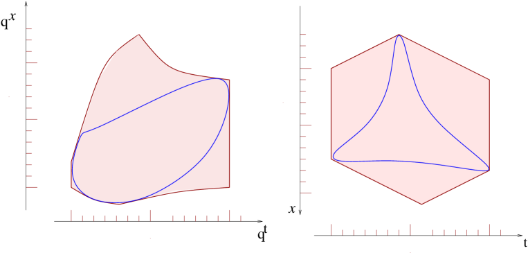 Figure 16: The envelope of the liquid region, is the smallest degree algebraic plane curve, tangent to the image of the hexagon under .
Recovering the spectral curve from the envelope:
Assume that we know the envelope , or, writing and , assume that we know the plane curve , i.e. an algebraic curve tangent to the boundaries of the image of under . Let us explain how to recover the full spectral curve .
Given the equation of the envelope (which is a multivalued algebraic function), one can choose locally as a local parameter.
One finds that the spectral curve is (at least in the domain of where can be chosen as a local parameter):
| (6-53) |
Therefore, knowing the envelope allows to recover the full spectral curve, i.e. the functions and also from eq. (6-35).
6.3.4 Small Asymptotic expansion
Now, suppose that we have found those functions, and that we have indeed found the correct spectral curve. The spectral curve is then the pair of functions , i.e., up to a symplectic transformation:
| (6-54) |
and we notice that and do not depend on , they depend only on , therefore we have .
And thus, from theorem 4.1, we have the full large asymptotic expansion:
Conjecture 6.2
A possible proof could follow the same ideas which we discussed in section 6.1.7 for .
6.4 Microscopic asymptotics
It is a truism to say that since our model is a matrix model, it has all the local universal behaviors of matrix models.
6.4.1 Zoom near a point
Let us choose a point anywhere in the plane (it can be in or outside the domain, or on the border).
Let us rescale and with some scaling parameter , with some exponents and , i.e. we write:
| (6-56) |
Also, on the spectral curve, we choose a point such that , and we rescale it by choosing a rescaled local parameter :
| (6-57) |
We rewrite the asymptotics of the functions and in terms of those rescaled variables:
| (6-58) |
If the exponents are well chosen, then the spectral curve , is a regular spectral curve (it has only branchpoints of square-root types). We call this curve, the blow up of the spectral curve near the point . In practice, finding the blow up is a rather trivial task, it merely consists in finding the first non-vanishing terms in the Taylor expansion near a point.
From [27], we have that the correlation functions :
| (6-59) |
behave at small like:
| (6-60) |
where are the “symplectic invariants” correlation functions of [27] associated to the spectral curve .
In other words, since the correlation functions are symplectic invariant correlators of a spectral curve , their local behavior is, to leading order, given by the symplectic invariant correlators of the blown up spectral curve. This theorem found in [27] is very easy to prove by recursion on and (see appedix B).
Therefore, it suffices to find the blown up spectral curve to characterize the leading behavior of the correlation functions near a point.
6.4.2 Airy kernel near regular boundaries of the liquid region
Near a regular point of the envelope , we have at and thus, we have a Taylor expansion in of the form:
| (6-61) |
where each has a regular Taylor expansion in . Let us rescale:
| (6-62) |
We have to the first few orders in :
| (6-63) |
We also have
| (6-64) |
and therefore
| (6-65) |
The blown up curve is thus:
| (6-66) |
which satisfies:
| (6-67) |
The spectral curves such that where is a polynomial of degree and is a polynomial of degree , appear in the so-called -minimal models, i.e. in the classification of conformal field theories [49, 20]. It has central charge . Here, this is the minimal model, with central charge , which is well known to be generated by the Airy differential system , and the correlation functions are determinants of the Airy kernel. It is also well known to be related to the Tracy-Widom law of extreme eigenvalues statistics [70].
6.4.3 Pearcey kernel near cusps
We have a cusp each time a pole disappears, generically a simple pole. Thus we have a Laurent expansion in starting at , and such that the residue of the pole vanishes at , i.e.:
| (6-68) |
and all the coefficients have a regular Taylor expansion near . Let us rescale and , to order , and up to constant terms, we have:
| (6-69) |
and generically, behaves like:
| (6-70) |
The blown up curve is thus:
| (6-71) |
and the local behaviors of correlation functions, are the correlation functions of that universal curve.
This is the spectral curve whose correlators are generated by the Pearcey kernel.
We thus recover the well known Pearcey kernel behaviour [71].
6.4.4 Critical points
If we consider a point on the boundary, such that more derivatives vanish, typically we find that the spectral curve behaves locally like:
| (6-72) |
It was shown in [27], that the correlation functions tend towards those of the reduction of the K-P hierarchy, i.e. the minimal model of central charge .
The model of central charge is called ”pure gravity”, the model of central charge is called Lee-Yang, The model of central charge is called the Ising model,… Their correlators are generated by determinantal formulae from a kernel involving the -system associated to a non-linear equation of Gelfand-Dikii type (Painlevé I is the Gelfand-Dikii equation for pure gravity ). Some details can be found in [20, 8].
6.4.5 Other local behaviors
Also, we expect that locally in the bulk of the liquid region, the behavior is given by the sine-kernel [10, 6, 43], and near vertical boundaries of the liquid region, we have , i.e. we expect the model, described by the Hermit kernel of the “birth of a cut” (see [13, 34]). And we also expect to find the ”Bead model” limit in the tentacles of the amoeba when is large, see [12].
However, these cases are such that the blown up curve is not regular, and we cannot directly apply the method of [27].
6.4.6 Arbitrary local behaviors
Then, one could easily invent some domains, for which a local blown up curve could be any spectral curve specified in advance, and by choosing sufficiently complicated domains one can obtain any limit law.
The classifications of all possible laws is more or less the classification of singularities of spectral curves, and it is more or less the classification of spectral curves themselves.
7 Examples
In this section, we illustrate our method by applying it to several classical examples, which were already studied in the literature with other methods. Here, however, we have a method to obtain not only the large size limit, but also all corrections to all orders.
7.1 The hexagon
Our domain is the hexagon of figure 17, with slopes .
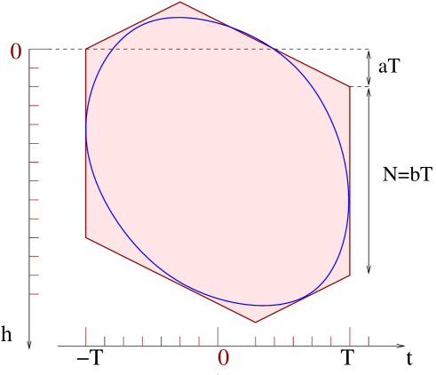 Figure 17: Domain for the hexagon.
We choose . We choose the weighs at all times. We write .
There is no defect, therefore we have , the reduced matrix integral is a 2-matrix model with an external field:
| (7-1) |
where is the fixed following matrix:
| (7-2) |
For , we can choose
| (7-3) |
7.1.1 The classical hexagon
We apply the recipe of section 6.1.5.
First, the domain has no hole, and we look for an algebraic curve of genus , therefore it can be parametrized by a uniformizing variable in the complex plane . Let us look for 2 rational fractions and , with 2 poles, and we write:
| (7-4) |
Up to a reparametrization of , we choose the poles to be at and . Moreover, we require that at the pole at disappears, and that at the pole at disappears, this implies that and and are of the form:
| (7-5) |
| (7-6) |
We define:
| (7-7) |
Then we find the coefficients by solving the following system:
| (7-8) |
We have 3 unknowns and 4 equations, but one can check that there are only 3 independent equations, and the system has a solution.
We easily find:
| (7-9) |
Envelope
The branchpoints are found from , and we find that there are two branchpoints:
| (7-10) |
That gives:
| (7-11) |
or explicitely
| (7-12) |
One can easily check that this is the equation of the ellipse tangent to all sides of the hexagon. See the ellipse in fig.17.
7.1.2 The quantum hexagon
Now consider , and write:
| (7-13) |
and we shall define the -numbers:
| (7-14) |
Let us now apply the recipe of section 6.3.2.
We write:
| (7-15) |
where and are rational fractions with two poles. Up to a reparametrization of , we choose the poles to be at and . Moreover, we require that at the pole at disappears, and that at the pole at disappears, this implies that and and are of the form:
| (7-16) |
We define:
| (7-17) |
Then we find the coefficients by solving the following system:
| (7-18) |
We have 3 unknowns and 4 equations, but one can check that there are only 3 independent equations, and the system has a solution. We find:
| (7-19) |
| (7-20) |


 Figure 18: The envelope of the hexagonal domain. The plots of eq. (7-21) are for the hexagon , , and for values of respectively .
Notice that the liquid region is convex only for close to .
Figure 18: The envelope of the hexagonal domain. The plots of eq. (7-21) are for the hexagon , , and for values of respectively .
Notice that the liquid region is convex only for close to .
Envelope
7.2 The cardiod
Consider the classical case . The domain is the one represented in figure 19. We assume , and .
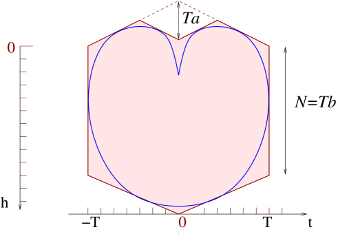 Figure 19: The domain of the cardioid. The envelope is a cardioid.
We find the spectral curve by applying the recipe of section 6.1.5.
Consider
| (7-22) |
where and are rational fractions with 3 poles.
Up to a reparametrization of , we choose the poles to be at . Moreover, we require that at the pole at disappears, at the pole at disappears, and at the pole at disappears. Moreover, since the domain has a symmetry , we choose and and of the form:
| (7-23) |
| (7-24) |
The symmetry is such that .
We write:
| (7-25) |
| (7-26) |
| (7-27) |
The coefficients are determined from the following system (we have written only the independent equations):
| (7-28) |
Those equations imply that:
| (7-29) |
| (7-30) |
| (7-31) |
And we have:
| (7-32) |
Envelope
Let .
Parametrically
| (7-33) |
| (7-34) |
One can check that it is the equation of the cardioid inscribed in the domain, see fig.19.
The same domain can also be considered in the quantum case, but we don’t do it here.
7.3 The trapezoid
Take , is the domain at and at . We choose the weights and with constant in time. We study the classical case .
Notice that , therefore the initial matrix is not fixed, it must have a potential satisfying conditions eq. (3-13) instead of eq. (3-14), but in fact it suffices to choose:
| (7-35) |


 Figure 20: The envelope of the trapezoidal domain. The plots are for .
Let us look for an algebraic genus zero spectral curve of minimal degree. First, notice that we have no cusp condition at . We thus need to have only 2 poles, let us say at and , and the pole at disappears at . Thus we write (with ):
| (7-36) |
That means
| (7-37) |
and
| (7-38) |
The coefficients can be determined by requiring that:
such that and .
such that and .
at .
The last condition implies and . Then, the 2 other conditions imply and .
Finally we find the following spectral curve:
| (7-39) |
| (7-40) |
| (7-41) |
The envelope of the liquid region is:
| (7-42) |
this is a parabola shifted by a straight line, and tangent to at least two of the trapezoid boundaries.
Notice that when , particles have the same probability to go upward or downward , and the spectral curve is symmetric with respect to . When is very small, the probability to go downward is very small, and therefore almost all the particles are in the solid region going upward, and the liquid region becomes a narrow region around the line . On the countrary, when is very large, the probability to go downward is very large, and almost all the particles are in the solid region going downward, and the liquid region becomes a narrow region around the line . See fig.21.
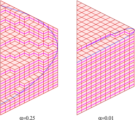 Figure 21: Typical self-avoiding particles model, or typical plane partitions in the trapezoid.
The tiling outside the liquid region is regular, it is frozen.
For small , the probability to go downward is very small, and therefore almost all the particles are in the solid region going upward, and the liquid region becomes a narrow region around the line .
Figure 21: Typical self-avoiding particles model, or typical plane partitions in the trapezoid.
The tiling outside the liquid region is regular, it is frozen.
For small , the probability to go downward is very small, and therefore almost all the particles are in the solid region going upward, and the liquid region becomes a narrow region around the line .
7.4 The Plancherel law
Let us choose a partition , and . we write:
| (7-43) |
we have:
| (7-44) |
Consider the domain , comprised between , and , and such that at the particles are at (in some sense the boundary is the trivial partition shifted by ), and at , the particles are at (the boundary is the partition ). See fig 22.
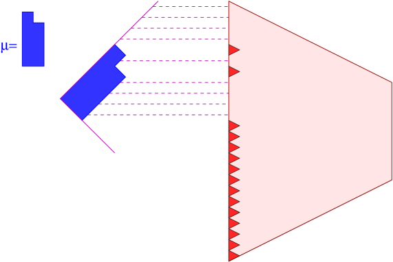 Figure 22: The domain for the Plancherel law. At time , we have , and at time we have .
Let us call the plane partitions generating function in this domain:
| (7-45) |
Let us define the ”Plancherel law” as the the limit :
| (7-46) |
It has been well known from a really long time [68], that:
| (7-47) |
and if , that reduces to the classical Plancherel law:
| (7-48) |
As a check of our matrix model approach, let us recover this classical result from the matrix model.
7.4.1 The classical Plancherel law
As presented in section 3, the domain is characterized by:
the matrix :
| (7-49) |
a potential at , which satisfies the conditions of eq. (3-14), we choose:
| (7-50) |
Notice that we have:
| (7-51) |
and thus:
| (7-52) |
and
| (7-53) |
Theorem 3.1, or more precisely its reduced version theorem 4.2, gives the relationship between the self-avoiding particles model partition function and the matrix model:
| (7-54) | |||||
| (7-55) |
i.e.:
| (7-56) |
And we can already guess, that in the large limit, the role of the ’s in the spectral curve is going to be subleading, i.e., to large leading order is going to be independent of .
In principle, our matrix model could be used to find the asymptotics of the Plancherel measure [60].
8 Obliged places and TSSCPPs
So far, we have considered a self-avoiding particles model with defects, i.e. forbidden places for the particles. Defects were introduced by choosing at the corresponding place .
One could also be interested in constrained self-avoiding particles model, where we want to oblige some places to be visitted at some given times. This cannot be achieved directly by tuning the potentials , but this can be achieved as follows.
8.1 Obliged places
We choose a potential such that at the place , i.e. we enforce a probability that the place can be visited. In other words, the contribution of self-avoiding particles configurations such that one particle visits will be proportional to , and the contribution of self-avoiding particles configurations such that no particle visits will be independent of (notice that no more than one particle can visit ). Therefore the partition function is made of two terms:
| (8-1) |
where is the partition function of self-avoiding particles configurations which visit . We have:
| (8-2) |
In other words, can be realized as some expectation value in our matrix integral. We write:
| (8-3) |
We have that:
| (8-4) |
More generally, if we want to have several obliged places , , we introduce a function for each of them.
| (8-5) |
Again, we have some arbitrariness in the choice of . The only requirements are:
and for integer, , we choose such that:
| (8-6) |
and arbitrary values everywhere else.
A possible choice could be:
| (8-7) |
but many other choices could also be made.
8.2 TSSCPP
An application of what precedes is the partition function for counting TSSCPP (Totally symmetric self-complementary plane partitions) see fig 23. Counting TSSCPP has become a famous combinatorics problem, due to its link with alternating sign matrices, Razumov-Stroganoff conjecture, Hecke algebras and qKZ relations [21, 4].
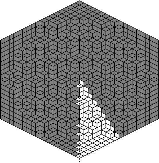 Figure 23: A TSSCPP, is a plane partition with all symmetries of the hexagon+ self complementarity (i.e. imagine that it is a pile of cubes within a big cube, then it must be equal to its complement).
A TSSCPP configuration is completely determined by a partition of th of the hexagon (the white region).
Figure 23: A TSSCPP, is a plane partition with all symmetries of the hexagon+ self complementarity (i.e. imagine that it is a pile of cubes within a big cube, then it must be equal to its complement).
A TSSCPP configuration is completely determined by a partition of th of the hexagon (the white region).
A TSSCPP configuration is completely determined by a partition of th of the hexagon.
In terms of a self-avoiding particles process, see fig. 24, this can be viewed as self avoiding particles jumping by , and such that particle has to follow a straight line after time :
| (8-8) |
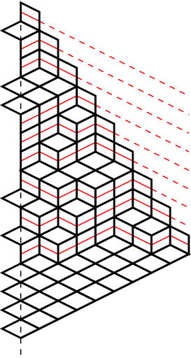 Figure 24: A plane partition of 1/12th of the hexagon, can be realized as a self-avoiding particles process such that if .
In other words, we have a self-avoiding particles process with some obliged positions. Also, we don’t fix the positions of the particles at time (although we could easily do it in our matrix model) .
Notice that if we fix at time , and if we oblige only at time , then the self-avoiding particles process necessarily evolves in a way such that if . In other words, it is sufficient to oblige only 1 position at each time: we oblige the position at time .
8.2.1 The matrix model
We choose for :
| (8-9) |
where the constant is such that .
We may also choose:
| (8-10) |
where the constant is such that .
For our matrix model, we choose the potential for all (there is no defect).
The TSSCPP partition function is thus realized by the matrix model:
| (8-12) | |||||
where we integrate an , and is not integrated upon. All matrices are of size .
8.2.2 Examples
:
| (8-13) |
| (8-14) |
:
| (8-16) | |||||
| (8-17) |
| (8-18) |
8.2.3 The spectral curve
Since we have chosen all , we have the same spectral curve as for the Trapezoid of section 7.3. Our partition function is computed as an expectation value.
| (8-20) | |||||
8.2.4 Fixed position at time t=0
If we want to fix the positions of particles at time , it suffices to introduce a potential
| (8-21) |
It would be interesting to relate those partition functions with fixed initial conditions for the particles, and see if we have some qKZ equations, and if they can be related to Alternating sign matrices partition functions.
It was already noted [72] that there is a matrix model formulation for the 6-vertex model counting Alternating sign matrices. It would be interesting to compare the spectral curve of the 6-vertex matrix model, and the spectral curve of the matrix model we introduced here.
9 Application to topological strings
Regarding the applications to algebraic geometry and topological strings, our method allows to see that Gromov-Witten invariants of the toric Calabi-Yau 3-folds with branes (called the topological vertex), are the symplectic invariants of their mirror’s spectral curve . In other words, we confirm that the ”remodelling the B-model” proposal of BKMP [11] holds for those toric CY 3-folds:
| (9-1) |
This claim is in the spirit of Dijkgraaf-Vafa conjecture, saying that B-model topological strings should be equivalent to some matrix model. Here, we have proved, that the topological vertex itself can be written as a matrix model.
In order to prove BKMP for general toric CY 3 folds, It remains to find a ”matrix-model way” to glue topological vertices together.
10 Conclusion
We have introduced a new formulation of self-avoiding particles model in statistical physics, or lozenge tilings, dimer models, or plane partitions, in terms of matrix models. Then we briefly discussed how to apply the rich technology of matrix models.
However, this is only a starting point, it is only a proposed framework, and we expect that exploiting the immense knowledge of matrix integrals developped since Wigner-Dyson-Mehta, we can find new consequences for self-avoiding particles model.
It should be possible to look at many extensions of this approach, for instance taking appropriate limits, it should be possible to apply this formalism to Dyson processes, or vicious walkers, and recover many results in the matrix model framework.
As an application to algebraic geometry, we have only found the ”topological vertex”, i.e. the building block for computing Gromov-Witten invariants of all toric CY 3-folds, but unfortunately, it is at the present time, not known how to perform the gluing of vertices, in the language of symplectic invariants of [27]. This question needs to be addressed.
Acknowledgments
We would like to thank Marcos Mariño for numerous discussions. We would also like to thank G. Borot, P. Di Francesco, A. Kashani-Poor, P. Ferrari, K. Mallick, M. Mulase, N. Orantin, A. Prats-Ferrer, S. Sheffield, C. Tracy, H. Widom, P. Zinn-Justin for useful and fruitful discussions on this subject. This work is partly supported by the Enigma European network MRT-CT-2004-5652, by the ANR project GIMP (Géométrie et intégrabilité en physique mathématique) ANR-05-BLAN-0029-01, by the ANR project GranMa (Grandes Matrices Aléatoires) ANR-08-BLAN-0311-01, by the Enrage European network MRTN-CT-2004-005616, by the European Science Foundation through the Misgam program, by the Quebec government with the FQRNT.
Appendix A Gamma-function and q-product
A.1 Gamma-function
The Gamma-function is such that:
| (1-1) |
If is a positive integer:
| (1-2) |
has poles at all negative integers:
| (1-3) |
We have:
| (1-4) |
Stirling formula:
| (1-5) |
where are the Bernouilli numbers.
| (1-6) |
A.2 q-product
The q-product is defined as an infinite product:
| (1-7) |
The function shares many similarities with the function , by replacing integers with numbers. It is a quantum -function. numbers are:
| (1-8) |
They tend to usual numbers in the limit .
If is an integer we have:
| (1-9) |
Stirling formula at small :
| (1-10) |
| (1-11) |
where is the Polylogarithme:
| (1-12) |
| (1-13) |
That is:
| (1-14) |
Appendix B Introduction to symplectic invariants
Here, we briefly recall the definition of symplectic invariants, but we refer the reader to [27, 28] for more details.
They were first introduced in [24, 15] and further formalized in [27], as a solution of the so called ”topological expansion” of matrix integrals. But then, in [27], they were defined as algebraic quantities for spectral curves, independently of the existence of an underlying matrix model.
B.1 Definition of symplectic invariants
Consider a spectral curve , where is a compact Riemann surface, and and are two analytical functions, such that and are meromorphic forms on .
The branchpoints are defined as the zeroes of :
| (2-1) |
We assume that the spectral curve is regular, i.e. we have a finite number of branchpoints, and they are simple branchpoints, which means that each is a simple zero of , and . This is equivalent to say that near , we have a square root behaviour:
| (2-2) |
Since we have a square root branchpoint near , this means that in the vicinity of , there exists on the other branch, i.e. :
| (2-3) |
is called the conjugate of near . It is defined only locally near branchpoints, and it is not necessarily defined globally.
On a Riemann surface , there exists a ”Bergman kernel”, i.e. a symmetric meromorphic 2-form, having a double pole, with no residue, on the diagonal, i.e. which behaves like:
| (2-4) |
where is any local parameter.
The Bergman kernel is unique if we also fix its periods , but this is not necessary for the definition of symplectic invariants. Let us assume that we have choosen one Bergman kernel .
Definition B.1
We define the following forms:
| (2-5) |
| (2-6) |
and by recursion for and , and if we denote collectively :
| (2-8) | |||||
where:
| (2-9) |
For , and , we define:
| (2-10) |
where is any function such that .
The ’s defined in this way are always symmetric meromorphic -forms, having poles only at branchpoints (except and ). And does not depend on the choice of integration constant for .
There is also a definition for and , but we refer the reader to [27].
B.2 Symplectic invariants of genus zero spectral curves
An interesting example is when is the complex plane . and are functions of a complex variable . In that case we have:
| (2-11) |
For example we have:
| (2-12) |
B.3 Examples of spectral curves and their symplectic invariants
Let us give a few examples of spectral curves:
The spectral curve defined by the functions , i.e. appears in the Weil-Petersson volumes of moduli spaces, its ’s are the Weil-Petersson volumes: , see [29].
The spectral curve defined by , i.e. is associated to the Airy kernel law, and to the universal behavior of extreme eigenvalues distribution, i.e. to the Tracy-Widom law [70]. The ’s of the Airy curve are equal to zero: .
The spectral curve , where is a polynomial of degree , is associated to the minimal model in conformal field theory (with central charge ), i.e. a reduction of the KdV hierarchy. Its ’s are related to the KdV Tau-function, and they can be computed by the asymptotic expansion of the solution of a Painlevé type equation (in fact the Gelfand-Dikii equation ). The case i.e. the minimal model is the Airy case. The case i.e. the minimal model is called pure gravity, and the case i.e. the minimal model is called Lee-Yang singularity.
Spectral curves of type appear in topological strings, where is a polynomial. More precisely, consider a Toric Calabi-Yau 3-fold . Through mirror symmetry [40], it has a mirror , which is also a toric Calabi-Yau 3-fold, and which is given by a submanifold of of equation where is a polynomial. The spectral curve , is defined as the singular locus of , which satisfies the equation . The ”remodelling the B-model” conjecture of BKMP [11], is that the generating function of Gromov-Witten invariants of genus of , is equal to the symplectic invariant of the spectral curve of the mirror:
| (2-13) |
This conjecture was proved in few cases, and in particular for the family of Hirzebruch manifolds (which include the connifold), see [26]. It was also partially proved for Seiberg-Witten theories [46], and for geometries [66].
B.4 Some properties of symplectic invariants
Let us now give a few properties of symplectic invariants. We refer the reader to [27, 28] for the general theory, and for proofs and details.
Properties:
Homogeneity: If we rescale , which we note , we have:
| (2-14) |
In particular that implies .
Symplectic invariance: if two spectral curves and are symplectically equivalent, i.e. if there is a map from to which sends one spectral curve to the other and conserves the symplectic form , then:
| (2-15) |
For instance we can change where is a rational function, or , or , … etc, without changing .
The with are not symplectic invariants, they change under symplectic transformations, but they change in a covariant way. For example is an exact form.
Variations: Consider an infinitesimal deformation of the spectral curve , such that is a meromorphic differential form on the spectral curve. Any meromorphic form is dual to a cycle on the curve, the duality pairing is realized through the Bergman kernel:
| (2-16) |
Then, the infinitesimal variation of and is given by:
| (2-17) |
The infinitesimal variation of is the case : .
Limits: Consider a one parameter family of spectral curves , such that at , the spectral curve becomes singular. Consider its blow up: , where the exponent is chosen such that the curve is regular. Then we have:
| (2-18) |
and more generally
| (2-19) |
This theorem is very useful, it gives the asymptotic behaviors. For instance, if we zoom near a regular branch point, the spectral curve always behaves like , i.e. , and we find the Airy law, and Tracy-Widom. Near an algebraic cusp singularity , we find the spectral curve of the minimal model of conformal field theories (of central charge ), which is a reduction of the KP hierarchy.
Thes are just a few of the properties satisfied by the ’s. See [27] for more. For instance there are also modular properties and holomorphic anomaly equations, Hirota equations, and diagrammatic representations.
Appendix C Solution of matrix models
Let us present a brief review about matrix models.
C.1 Generalities on the solution of matrix models
Consider a matrix integral of type:
| (3-1) |
where is the set of normal matrices having their eigenvalues on contour , and where is not integrated upon.
If one wants to find a large expansion of , the answer, is that one has first to compute the ”spectral curve” (defined below), then, in [33], it is proved that:
Theorem C.1
If is the spectral curve associated to potentials and paths , and if has a large expansion of the form
| (3-2) |
then, the coefficient is the symplectic invariant of degree of the spectral curve . Symplectic invariants of a spectral curve were defined and introduced in [27].
We shall explain the meaning of this theorem below in further details. We shall explain how to compute the spectral curve of a matrix model, and how to compute its symplectic invariants . We recall the definition of symplectic invariants in appendix B.
Let us just mention that finding the spectral curve is rather automatic, it is mostly an algebraic task, and for most examples the spectral curve is a rather simple object. Here, we have the the spectral curves of Kenyon-Okounkov-Sheffield [48].
Then, computing the symplectic invariants of a spectral curve, is rather easy. The definition of symplectic invariants [27] involves computing residues of rather standard functions (exponentials, logs, rational functions, …), and can be completely automatized, see appendix B. It is really an efficient method. For example can often be computed by hand. Moreover, symplectic invariants satisfy many properties, which make them really convenient to use, for example there are formulae for computing their derivatives with respect to any parameter, and formulae for finding their limits near singularities.
C.2 Generalities about loop equations
Loop equations are obtained by integration by parts in the matrix integral, or equivalently, by writing that an integral is invariant under change of variable. For example, assume that we make an infinitesimal change of variable in eq. (3-1):
| (3-3) |
one finds the Jacobian to first order in :
| (3-4) |
Writing that the integral is invariant to first order in implies:
| (3-5) | |||||
| (3-6) |
Similarly, by considering other appropriate changes of variables, one can write a family of relationships of the type eq. (3-5) between expectation values, this was done systematically in [33].
Instead of considering expectation values of powers , is is more convenient to group them in a formal generating function . This leads to introduce:
| (3-7) |
(where the subscript means the cumulant, or connected part). Since we made the hypothesis that there exists a large expansion we write:
| (3-8) |
The problem consists in finding a family of relationships among those quantities, and which allow to find the solution, i.e. compute all of them. This was done in [33, 32].
The result of [33], is that the ’s are the n-forms of theorem C.1, i.e. the ’s of [27], and where the spectral curve is .
In some sense, can be viewed as the ”large ” limit of the resolvent of the matrix (the first matrix in the chain eq. (3-1)), it is often called the ”equilibrium distribution of eigenvalues of ”, but one should take this denomination with some care. Indeed, can be shown to be the ”weak” large limit of the resolvent, for some potentials (in particular in the potentials don’t depend on ), and some integration paths , but this is probably wrong in general. In fact, in our case, the potentials do depend on , and saying that the spectral curve is the ”large ” limit of the resolvant is slightly wrong (and at least one needs to make precise the notion of large limit).
The only correct definition of the spectral curve, which corresponds to theorem C.1, is that , is the first term in the formal large expansion, doing as if the potentials were independent of .
Working to order in the expansion eq. (3-8) within the loop equations, is formally equivalent to replacing expectation values of product of traces, by product of expectation values of each trace (indeed, the connected part comes with a factor , whereas the non-connected term, i.e. the factorized term comes with a factor , i.e. all terms which are not disconnected don’t contribute to the highest power of ):
| (3-9) |
This formal manipulation allows to find an equation which determines the spectral curve .
C.3 Spectral curve of the chain of matrices
C.4 General case
The spectral curve of a matrix integral of type eq. (3-1):
| (3-10) |
is characterized by a set (see [32, 33]) of analytical functions of a variable ( belongs to a Riemann surface ). There is one such analytical function for each matrix , of the chain, plus one additional function at the end of the chain. Let us call them:
| (3-11) |
Those functions are completely determined by the following system of equations:
| (3-12) |
and
| (3-13) |
together with the conditions:
has simple poles at the values of such that is an eigenvalue of . Let us call , the value of such that the eigenvalue of . Then we have in the vicinity of :
| (3-14) |
The function , is analytical outside of the cuts , the endpoints of the cuts being zeroes of . Near (only in the physical sheet), we have:
| (3-15) |
the genus of the Riemann surface , and the period integrals on non-contractible cycles of , are related to the choice of contours in the matrix integral eq. (3-10). The following quantity is called ”filling fraction”
| (3-16) |
and it is such that is the number of eigenvalues of contained in the domain surrounded by the projection in of the cycle by the application .
More generally, is the number of eigenvalues of contained in the projection in of the cycle by the application .
Finding the spectral curve for arbitrary potentials and arbitrary contours can be extremely tedious. However, here we are interested in formal matrix integrals, which are defined as formal power series expansions in some formal parameter, and in particular, the spectral curve we are looking for, must also be found as a formal power series. In particular, the genus is the genus of the spectral curve when we send the formal parameter to , and in general that simplifies the computation of the spectral curve a lot. Very often the genus is in fact zero.
C.4.1 Topological expansion
When we have determined the spectral curve , i.e. the two functions and :
| (3-17) |
we have:
| (3-18) |
It is then useful to use the symplectic invariance of the ’s.
Consider the following spectral curves:
| (3-19) |
Due to eq. (3-12), we have:
| (3-20) |
i.e. all the spectral curves are symplectically equivalent:
| (3-21) |
and therefore, the theorem of symplectic invariance of the ’s [27, 30] gives :
| (3-22) |
In other words, the ’s can be computed with the spectral curve where and are any two consecutive , we don’t need to choose the pair .
C.4.2 Densities and correlation functions
For the general chain of matrices, the ’s were defined as the Stieltjes transforms of the density correlation functions of the first matrix in the chain, i.e. the resolvents eq. (3-7). The densities can be recovered by taking the discontinuities:
| (3-23) |
where
| (3-24) |
We recall that the spectral curve used to compute here, is the spectral curve , and the ’s are not invariant under symplectic transformations.
However, just by applying eq. (2-17), one can see that, for any matrix of the chain, one has that the density of eigenvalues of :
| (3-25) |
is given by:
| (3-26) |
Therefore, the density of eienvalues of each matrix of the chain, can be computed to all orders in the large expansion, using the ’s defined in [27].
In the general chain of matrices, the support of the densities must be related to the integration paths ’s: One defines the support of densities as the loci where densities are real. The supports of densities, together with their analytical continuations, must be homologicaly equivalent to the integration paths ’s. And saying that the paths are steepest descent paths, is more or less equivalent to saying that the densities must be real and positive on their supports, and times the analytical continuation of the densities, along the analytical continuations of the supports, must be real and strictly positive (stability condition). This is a highly non trivial condition in general.
Fortunately, for formal matrix integrals, defined as formal power series in a formal parameter, the small limit of the parameter often gives a very simple matrix model, with a very simple spectral curve, and it is often easy to check positivity to leading order, and then, that the formal power series expansion does not destroy the supports and positivity.
References
- [1] M Adler, P van Moerbeke, “The spectrum of coupled random matrices”, Annals of Mathematics, 1999.
- [2] D.J. Aldous, P. Diaconis, Longest increasing subsequences: from patience sorting to the Baik-Deift-Johansson theorem, Bull. Amer. Math. Soc. 36 (1999), 413-432.
- [3] M. Aganagic, A. Klemm, M. Mariño, C. Vafa, The topological vertex, hep-th 0305132.
- [4] G. Andrews, Plane partitions. V. The TSSCPP conjecture, J. Combin. Theory Ser. A 66 (1994), no. 1, 28 39.
- [5] J. Baik, E.M. Rains, Symmetrized random permutations, Random Matrix Models and Their Applications, vol. 40, Cambridge University Press, 2001, pp. 1-19.
- [6] J. Baik, P. Deift, K. Johansson, On the distribution of the length of the longest increasing subsequence of random permutations, Journal of AMS, 12 (1999), 1119 1178.
- [7] K. Behrend, Gromov-Witten invariants in algebraic geometry, Invent. Math. 127 (1997), 601 617.
- [8] M. Bergère, B. Eynard, Determinantal formulae and loop equations, math-ph: arxiv.0901.3273.
- [9] N. M. Bogoliubov, Determinantal Representation of the Time-Dependent Stationary Correlation Function for the Totally Asymmetric Simple Exclusion Model, SIGMA 5 (2009), 052, arXiv:0904.3680.
- [10] A Borodin, A Okounkov, G Olshanski, Asymptotics of Plancherel measures for symmetric groups, Journal of the American Mathematical Society, 2000 - ams.org.
- [11] V. Bouchard, A. Klemm, M. Mariño, S. Pasquetti, Remodelling the B-model, hep-th 0709.1453.
- [12] C. Boutillier, The bead model and limit behaviors of dimer models, arXiv:math/0607162.
- [13] E. Brezin and S. Hikami, Universal singularity at the closure of a gap in a random matrix theory, cond-mat/9804023. Phys. Rev. E (3) 57 (1998), no. 4, 4140 4149.
- [14] J. Bryan and R. Pandharipande, The local Gromov-Witten theory of curves. math.AG/0411037.
- [15] L. Chekhov and B. Eynard, Hermitean matrix model free energy: Feynman graph technique for all genera, JHEP 0603, 014 (2006) [arXiv:hep-th/0504116].
- [16] H. Cohn, M. Larsen, and J. Propp, The shape of a typical boxed plane partition, New York J. Math. 4 (1998), 137 165, arXiv:math/9801059.
- [17] P. Deift, T. Kriecherbauer, K. T-R McLaughlin, S. Venakides, X. Zhou, “Uniform asymptotics for polynomials orthogonal with respect to varying exponential weights and applications to universality questions in random matrix theory”, Comm. Pure and applied Maths., Vol 52, 1335-1425, 1999.
- [18] Derrida, An exactly soluble non-equilibrium system: the asymmetric simple exclusion process, Phys. Rep. 301, 65, (1998).
- [19] B. Derrida, M. R. Evans, V. Hakim, V. Pasquier, 1993, Exact solution of a 1D asymmetric exclusion model using a matrix formulation, J. Phys. A: Math. Gen. 26, 1493.
- [20] P. Di Francesco, P. Ginsparg, J. Zinn-Justin, 2D Gravity and Random Matrices, Phys. Rep. 254, 1 (1995).
- [21] P. Di Francesco, Totally symmetric self-complementary plane partitions and the quantum Knizhnik-Zamolodchikov equation: a conjecture, J. Stat. Mech. Theory Exp. (2006), no. 9, P09008, 14 pp., arXiv:cond- mat/0607499.
- [22] P. Di Francesco, P. Zinn-Justin, Around the Razumov-Stroganov conjecture: proof of a multi-parameter sum rule, arXiv:math-ph/0410061.
- [23] P. Di Francesco, P. Zinn-Justin, J.-B. Zuber, Determinant Formulae for some Tiling Problems and Application to Fully Packed Loops, arXiv:math-ph/0410002.
- [24] B. Eynard, “Topological expansion for the 1-hermitian matrix model correlation functions,” arXiv:hep-th/0407261.
- [25] B. Eynard, “Formal matrix integrals and combinatorics of maps,” arXiv:math-ph/0611087.
-
[26]
B. Eynard, All orders asymptotic expansion of large partitions,
math-ph: arxiv.0804.0381. - [27] B. Eynard and N. Orantin, “Invariants of algebraic curves and topological expansion”, arXiv:math-ph/0702045.
- [28] B. Eynard and N. Orantin, Algebraic methods in random matrices and enumerative geometry, math-ph: arxiv.0811.3531.
- [29] B. Eynard, Recursion between Mumford volumes of moduli spaces, math-ph: arXiv:0706.4403.
- [30] B. Eynard and N. Orantin, Topological expansion of mixed correlations in the hermitian 2 Matrix Model and symmetry of the algebraic invariants, math-ph/arXiv:0705.0958, to appear in J.Phys A.
- [31] B. Eynard, M.L. Mehta, Matrices coupled in a chain: eigenvalue correlation, Journal of Physics A 19 (1998) 4449, arxiv: cond-mat/9710230.
- [32] B. Eynard, Master loop equations, free energy and correlations for the chain of matrices, JHEP11(2003)018, hep-th/0309036.
- [33] B. Eynard, A. Prats Ferrer, Topological expansion of the chain of matrices, math-ph: arxiv.0805.1368.
- [34] B. Eynard, Universal distribution of random matrix eigenvalues near the “birth of a cut” transition, math-ph/0605064, JSTAT, Theory and Experiment P07005 (2006) P07005.
- [35] P. L. Ferrari, M. Praehofer, One-dimensional stochastic growth and Gaussian ensembles of random matrices, proceedings of ”Inhomogeneous Random Systems 2005”, Markov Processes Relat. Fields 12 (2006) 203-234, arXiv:math-ph/0505038.
- [36] Patrik L. Ferrari, Polynuclear growth on a flat substrate and edge scaling of GOE eigenvalues, Comm. Math. Phys., 252 (2004), 77-109, arXiv:math-ph/0402053.
- [37] IM. Gessel, X. Viennot, Determinants, paths, and plane partitions, preprint, 1989 - 132.180.197.15.
- [38] O. Golinelli, K. Mallick, 2006, The asymmetric simple exclusion process : an integrable model for non-equilibrium statistical mechanics, J. Phys. A: Math. Gen. 39 12679.
- [39] Harish-Chandra, Amer. J. Math. 79 (1957) 87-120.
- [40] K. Hori, S. Katz, A. Klemm, R. Pandharipande, R. Thomas, C. Vafa, R. Vakil, E. Zaslow, AMS, Providence, 2003.
- [41] C. Itzykson and J.-B. Zuber, Jour. Math. Phys. 21 (1980) 411.
- [42] K. Johansson, The arctic circle boundary and the Airy process, Ann. Probab. 33 (2005), 1-30.
- [43] K. Johansson, The longest increasing subsequence in a random permuta- tion and a unitary random matrix model, Math. Res. Lett., 5 (1998), no. 1-2, 63 82.
- [44] Kasteleyn, P. W. (1961), ”The statistics of dimers on a lattice. I. The number of dimer arrangements on a quadratic lattice”, Physica 27 (12): 1209 1225, doi:10.1016/0031-8914(61)90063-5.
- [45] P. Kasteleyn, Graph theory and crystal physics, Graph Theory and Theoretical Physics, Academic Press, London, 1967, pp. 43 110.
- [46] A. Klemm, P. Sulkowski, Seiberg-Witten theory and matrix models, eprint arXiv:0810.4944.
- [47] R. Kenyon, Local statistics of lattice dimers, Ann. Inst. H. Poincaré Probab. Statist. 33 (1997), no. 5, 591 618.
- [48] R. Kenyon, A. Okounkov, S. Sheffield, Dimers and Amoebae, Annals of mathematics, Vol. 163, N 3,2006 ,1019-1056, arXiv:math-ph/0311005.
- [49] V.A. Kazakov, I. Kostov, A.A. Migdal, ”Critical properties of randomly triangulated planar random surfaces”, Physics Letters B, 1985.
- [50] C. Krattenthaler, “Generating functions for plane partitions of a given shape”, manuscripta mathematica, vol 69, 1, 1432-1785, 1990.
- [51] T.M. Liggett, Coupling the simple exclusion process, Ann. Probab. 4 (1976), 339-356.
- [52] M. Mariño, “Les Houches lectures on matrix models and topological strings,” arXiv:hep-th/0410165.
- [53] M. L. Mehta, “A method of integration over matrix variables”, Comm. Math. Phys., vol 79, 3, 327-340, 1981.
- [54] M.L. Mehta, Random Matrices, 3rd edition, (Academic Press, New York, 2004).
- [55] D. Maulik, A. Oblomkov, A. Okounkov, R. Pandharipande, Gromov-Witten/Donaldson-Thomas correspondence for toric 3-folds, arXiv:0809.3976.
- [56] A. Neitzke and C. Vafa, “Topological strings and their physical applications,” arXiv:hep-th/0410178.
- [57] N. Nekrasov, A. Okounkov, Seiberg-Witten Theory and Random Partitions, hep-th/0306238.
- [58] A. Okounkov, N. Reshetikhin, C. Vafa, Quantum Calabi-Yau and Classical Crystals, arXiv:hep-th/0309208.
- [59] A. Okounkov and N. Reshetikhin, Correlation function of Schur process with application to local geometry of a random 3-dimensional Young diagram, J. Amer. Math. Soc. 16 (2003), no. 3, 581 603, arXiv:math.CO/0107056.
- [60] A. Okounkov, Asymptotics of Plancherel measures for symmetric groups, Journal of American Mathematical Society, Vol 13, 3, 481-515.
- [61] A. Okounkov, Random surfaces enumerating algebraic curves, hep-th 0412008.
- [62] A. Okounkov and R. Pandharipande, Gromov-Witten theory, Hurwitz numbers, and matrix models, I, math.AG/0101147.
- [63] M. Prähofer and H. Spohn, Universal Distributions for Growth Processes in 1+1 Dimensions and Random Matrices, Phys. Rev. Lett. 84, 4882 (2000).
- [64] G. de B. Robinson, ”On representations of the symmetric group,” Amer. J. Math. 60 (1938), 745 760.
- [65] C. Schensted, Longest increasing and decreasing subsequences, Canad. J. Math., 13, 1961, 179-191. MR 22:12047
- [66] P. Sulkowski, “Matrix models for 2* theories”, arXiv:0904.3064.
- [67] K. Takasaki, Integrable structure of melting crystal model with two q-parameters, arxiv:0903.2607 [math-ph].
- [68] A. Vershik and S. Kerov, Asymptotics of the Plancherel measure of the symmetric group and the limit form of Young tableaux, Soviet Math. Dokl., 18, 1977, 527 531.
- [69] A. Vershik, Statistical mechanics of combinatorial partitions and their limit configurations, Func. Anal. Appl., 30, no. 2, 1996, 90 105.
- [70] C. A. Tracy and H. Widom, Level-spacing distributions and the Airy kernel, Commun. Math. Phys., 159, 1994, 151 174.
- [71] C. Tracy and H. Widom, The Pearcey Process, math.PR/0412005.
- [72] P. Zinn-Justin, Six-vertex model with domain wal l boundary conditions and one-matrix model, Phys. Rev. E 62 (2000), no. 3, part A, 3411 3418, arXiv:math- ph/0005008 .