A Markovian Model Market - Akerlof’s Lemmons and the Asymmetry of Information

Abstract

In this work we study an economic agent based model under different asymmetric information degrees. This model is quite simple and can be treated analytically since the buyers evaluate the quality of a certain good taking into account only the quality of the last good purchased plus her perceptive capacity $\beta$. As a consequence the system evolves according to a stationary Markovian stochastic process. The value of a product offered by the seller increases with quality according to the exponent $\alpha$, which is a measure of technology. It incorporates all the technological capacity of production systems such as education, scientific development and techniques that change the productivity growth. The technological level plays an important role to explain how the asymmetry of information may affect the market evolution in this model [3]. We observe that, for high technological levels, the market can control adverse selection. The model allows us to compute the maximum asymmetric information degree before market collapse. Below this critical point the market evolves during a very limited time and then dies out completely. When $\beta$ is closer to 1 (symmetric information), the market becomes more profitable for high quality goods, although high and low quality markets coexist. All the results we obtained from the model are analytical and the maximum asymmetric information level is a consequence of an ergodicity breakdown in the process of quality evaluation.

, , and ,

1 Introduction

There is an increasing interest in microscopic models to investigate the mechanism that drives the market [1, 2, 6]. In particular, researchers have focused on analytical and simple models that are able to capture some real aspects of the economic activity.

Akerlof analyzed in [1] the impact of asymmetric information on the market. Agents trade in the market because they share mutual benefits. However, when the information asymmetry increases, high quality goods drop out from market and only low quality goods can be traded, a situation called adverse selection.

Adverse selection is characterized as pre-contractual opportunistic behavior, since agents act in order to obtain more advantages, given the market conditions and information available on the contracts that regulate their commercial relations. Rules established in such contracts end up attracting more intensely those agents that it should repel (for example, the case of health insurance, which attracts more sick than healthy individuals).

In the simple model proposed by Y-C Zhang [4], Arkelof’s market failure is a special case. He revisited supply and demand laws by setting quality and imperfect information as the key ingredients. By varying continuously the information asymmetry parameter one observes two regimes. For some intermediate level of asymmetry consumers’ benefits and firms’ profits approach the maximum. In this case, both cooperate and firms invest in educating consumers to identify their goods’ qualities. After this maximum benefits still increase while profits decrease and consumers and producers are in conflict. One solution for this dilemma is product innovation.

Recently, Wang et. al [2] introduced an agent based model to address the impact of asymmetric information on the market evolution. They showed the emergence of adverse selection from the simulation of a very simple markovian model. For instance, the market of used goods is not completely explained in terms of asymmetric information [3]. To improve market understanding, it was introduced another variable called valuation ratio, defined as the gap between buyers’ valuation (consumers’ willingness to pay) and the sellers’ valuation (firms’ cost) about the same good under the situation of complete information. The coexistence of high and low quality is a consequence of a trade-off between buyers’ perception of product quality and large valuation ratio.

It is worth to note that in the model we do not take into account the quantity of produced goods. From the microeconomic theory, we know that it is relevant to understand the supply and demand law. However, as noted by Zhang [4], products in the economy are more complex. Both quality and information play important roles in the understanding of how market behaves. The consumer’s perception depends on the amount of information available, becoming crucial for the agent when it comes to evaluate the good and make decision.

We are not considering here the produced quantity. The relevant aspect is only the product quality. Since in this study the amount of goods produced do not matter, the model is suitable to describe the economy of information (software companies, e-books, films production, and so for). In such context the key feature are abstract aspects (knowledge, design and creativity) and the replication cost is cheap (or the marginal cost is constant). Consequently, the prototype is cheap to replicate but hard to define the selling price, which depends on the product quality and the ability of consumers to recognize it.

In this work, we study a market model discussed above under some fixed technological production levels and several asymmetric information degrees [1, 2]. The model is developed on consumer’s and firm’s perceptions of value attributable to the good, regardless the market prices.

2 Model

There are $N_{s}$ sellers that offer goods with different integer quality equally distributed in the range $[1,...,\kappa]$ and $N_{b}$ buyers which have access to all goods in the market. At each step the buyer $i$ chooses one seller at random and evaluates the quality $q$ she is buying according to the expression

$$q_{i}=\beta k+\left(1-\beta\right)k_{a}^{i},$$ (1)

where $\beta\in[0,1]$ is the degree of asymmetric information, $k$ is the quality of goods informed by the seller to the consumers and $k_{a}^{i}$ is the quality of the last item purchased by the agent $i$. The buyer recognizes the real quality of the item (the one attached by the seller) only after purchasing it, and this quality is used as the next $k_{a}^{i}$. For $\beta=1$ the information is both perfect and symmetric, that is, the two groups share the same quality perception. As $\beta$ decreases the consumers are no longer able to precisely identify the products’ quality (though they are not aware of it). The asymmetry of information emerges from the different perceptions between sellers and buyers about the same product, and the buyers’ inability to assign the product its true quality raises an imperfect state of information (although it is still perfect on the seller’s side). The asymmetry reaches its maximum when $\beta$ equals zero, making it impossible for the buyers to have any idea about the quality of the good she is purchasing.

Consumers and firms may disagree on how much a good is worth (actually they do), so it is not expected they would agree on a value assigned to it or even on how much should cost a difference in the quality of a product. In this sense, we consider two distinct ways for buyers and sellers to assign a value to the product, depending on its quality. The consumers have a valuation function

$$V_{i}^{b}(k;k_{a}^{i})=Aq_{i},$$ (2)

where $A$ is a rate of the buyer‘s willingness to pay, while the sellers compute the minimum value of their goods by taking into account the actual manufacturing technological state of the economy $\alpha$ and the monetary scale of sales $B$ via

$$V^{s}\left(k\right)=Bk^{\alpha},$$ (3)

with $\alpha>0$ and $B>0.$ A commercial transaction occurs only when

$$V^{b}(k;k_{a}^{i})\geq V^{s}(k),$$ (4)

otherwise the buyer chooses randomly another seller in the next step.

The consumers’ willingness to pay is linked to the value she concedes to the good, which includes the valuation of a set of attributes she values most at acquisition of a certain type of product or service (for example, durability, quality, color, taste, size, shape, sophistication, luxury, among others). If the sum of those valuations given to the good falls below the firms production cost (that is, in principle, the minimum value that the firm is willing to accept to sell the good, which includes the firms’ opportunity costs), no trade transaction occurs. No consumer will accept to pay a price higher than the value established by her willingness to pay, since her perception of the attributes the good will provide do not compensate the utility of the money she is giving up.

When one computes the marginal value $\partial_{k}V^{s}(k)$, three regimes may result according to the $\alpha$ parameter value. For $\alpha<1$ the technological state of the economy is marginally more efficient, i.e, cheaper than the case of $\alpha>1$ where the derivative decreases as the quality increases (the marginal value is constant when $\alpha=1)$. It is possible to associate $\alpha$ with the economy state of technology because a seller may produce the same product with a lower cost by decreasing the $\alpha$ value.

In a bargaining trading process the price will be somewhere between the consumer‘s willingness to pay $V^{b}\left(k;k_{a}\right)$ and the firm‘s cost $V^{s}\left(k\right)$. The discussion on the differences between price and value involves lots of controversy, including the differentiation between value in use and value in exchange, according to Adam Smith [6], ”no trade occurs if the value in use of a good is lower than its value in exchange”. That is, whenever a trade occurs, the value in use (utility of the good for the consumer) is usually significantly higher than value in exchange (market price), and the later should be at least equal to or higher than the production cost. Based on this observation we define the relative profit as $\gamma=\frac{V^{b}}{V^{s}}$ just to avoid introducing a sophisticated price dynamics model.

Our focus is on the impact of asymmetric information under fixed technological level in the evolution of the market. The buyer’s quality evaluation mechanism follows a markovian process since only the more recent state is relevant for computing the next quality. We study the maximum asymmetric information for the market to reach a stationary state. Also, we discuss the consumer‘s average observed quality for several asymmetric information levels and the average number of transactions per round.

3 The stationary probability distribution of the traded quality

In each round a buyer chooses one seller at random, who will offer her a product of quality $k$. The probability $p_{v}\left(k,k_{a}\right)$ for the transaction to occur is given by

$$p_{v}\left(k,k_{a}\right)=Pr\left[V^{b}\left(k,k_{a}\right)\geq V^{s}\left(k\right)\right]=Pr\left[\beta k+\left(1-\beta\right)k_{a}\geq\lambda{k}^{\alpha}\right],$$ (5)

where $\lambda=B/A$ and $k_{a}$ is the last product purchased by the buyer. For this buyer’s next round, her $k_{a}$ will either be the same or change to $k$, depending on the result of this transaction. In this way one can describe the buyer’s behavior as a stochastic process, where her state $n$ is defined by the quality of her last purchased good, which may remain the same if condition (4) if not fulfilled (or if she is trying to purchase the same quality) or undergo a transaction $n\rightarrow m$ whenever she tries to acquire a new good with quality $m$. The transition between states must be probabilistic since the new seller is chosen at random, and the use de Heaviside’s step function $\Theta\left(x\right)$ guarantees that only accessible states are reached. Describing the transition probabilities as

$$Pr\left(n\rightarrow m\right)=\frac{1}{N_{s}}\Theta\left[\beta m+\left(1-\beta\right)n-\lambda m^{\alpha}\right],$$ (6)

$$Pr\left(n\rightarrow n\right)=\frac{1}{N_{s}}\Theta\left(n-\lambda n^{\alpha}\right)+\frac{1}{N_{s}}\sum_{w=1}^{N_{s}}\Theta\left[\lambda w^{\alpha}-\beta w-\left(1-\beta\right)n\right].$$ (7)

one can define a transition matrix $T$ with elements $T_{nm}=Pr\left(m\rightarrow n\right)$, and set a vector $\mathbf{P}_{t}$ describing the probability of the buyer to be found in each state of the system. The expression for the stochastic process given by $\mathbf{P}_{t+1}=T\mathbf{P}_{t}$, where the stationary solution $\mathbf{\Pi}=T\mathbf{\Pi}$ may be obtained by either diagonalizing the $T$ matrix (in order to find the eigenvector with eigenvalue equal to unity) or numerically by iterating the equation until the convergence is reached.

The $\alpha$ parameter plays an important role in the model because it affects the state of the economy depending on the values it may assume. By considering a condition when a trade can not occur ($V^{b}<V^{s}$) and $\beta=1$, it is possible to find out the conditions for the market to exist. If $\alpha\geq 1$, then we must have $\lambda\leq 1$, as for the case when $\alpha<1$ the condition $\lambda\leq\kappa^{1-\alpha}$ must hold. Given that $\lambda$ satisfies either of this conditions, three different market pictures arise, depending on the technological state $\alpha$: $\alpha>1$ gives rise to a forbbiden high quality region above $\hat{k}=\lambda^{\frac{1}{1-\alpha}}$, independently of $\beta$; for $\alpha<1$ a forbbiden low quality region below $\hat{k}$ emerges when $\beta=1$, but it becomes allowed as $\beta$ decreases; if $\alpha=1$ no prohibitive region appears.

In Fig.1 we show the stationary solution $\Pi\left(k\right)$, with $\alpha=\frac{1}{2}$ and $\lambda=10$, for several asymmetric information levels $\beta$. For perfect information ($\beta=1$) there is no transaction below $k\leq\lambda^{2}=100$. Thus, the distribution probability $\Pi$ is uniform in the interval $\left[\lambda^{2},\dots,\kappa\right]$, the buyers can purchase any goods available in the market because there is no budget constraint in this model. When the asymmetry of information arises, but is still close to 1, it becomes possible to purchase products at a quality lower than $\lambda^{2}$. For $\beta$ values much lower than 1, the distribution probability $\Pi$ has a peak in this lowest quality region indicating the adverse selection phenomena.

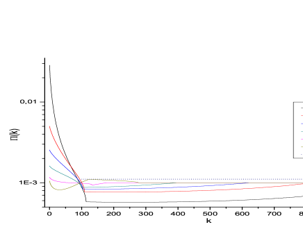
Figure 1: Probability distribution $\Pi$ as a function of quality $k$. Information asymmetry rises the probability of negotiation for low quality

In the stationary state, the probability $\Pi(k)$ for a buyer to be on the $k^{th}$ state may be associated with the probability of his last purchased item be $k$, since $\mathbf{P}_{t+1}=\mathbf{P}_{t}=\mathbf{\Pi}$. This allows one to calculate the vendor’s probability to sell a product to one unspecified buyer using (5),

$$p_{k}=\sum_{k^{\prime}=1}^{\kappa}p_{v}\left(k,k^{\prime}\right)=\sum_{k^{\prime}=1}^{\kappa}\Theta\left[\beta k+\left(1-\beta\right)k^{\prime}-\lambda k^{\alpha}\right]\Pi\left(k^{\prime}\right).$$ (8)

that is, the probability of the seller $k$ to perform a transaction given that she was chosen by one buyer.

It is worth to note that, for fixed $\alpha<1$ there is a maximum asymmetric information degree for the market to exist given by some critical value $\beta_{c}$. This points out to the condition for the occurrence of Akerlof‘s lemmon market: association of low quality goods with an environment of high information asymmetry leads to low willingness to pay by consumers and high production cost by firms ($\lambda>1$). For instance, taking $\lambda=10$ we obtain $\beta_{c}=0.319$. In what follows we run all the simulation for $\beta\in\left[0.32,\dots,1\right]$. To get an analytical curve for $\beta_{c}$ we observe that for a buyer in the state $k_{a}=1$ the trade condition below a certain asymmetric information degree $\beta_{c}$ is never satisfied, even if the buyer meets the highest quality goods in the market (which she values the most), and the market evolves to extinction. In other words, $k_{a}=1$ becomes an absorbing state, and all agents (buyers) will eventually collapse to it. Taking $V^{b}\left(\kappa,1\right)=V^{s}\left(\kappa\right)$ and $\beta=\beta_{c}$, we get

$$\beta_{c}\left(\kappa\right)=\frac{\lambda\kappa^{\alpha}-1}{\kappa-1}.$$ (9)

Also if $V^{b}\left(\kappa,1\right)=V^{s}\left(\kappa\right)$ holds, then for any state $n>1$ we have $V^{b}\left(\kappa,n\right)\geq V^{s}\left(\kappa\right)$, which means that if $k_{a}=1$ is not an absorbing state then there are no absorbing states in the system. In this way, the maximum asymmetric information level is a consequence of an ergodicity breakdown in the process of quality evaluation.

The completeness of the system (accessibility of all states) is guaranteed if the condition

$$\kappa\geq\frac{\lambda-\beta}{1-\beta}$$ (10)

holds, but it’s only valid in the region $\beta<1$, since for $\beta=1$ the existence of states where the buyer’s valuation is below the seller’s level is not allowed.

From equation (9), one may see that there is an interval where the parameter $\lambda$ has some interest. Noting that $0\leq\beta\leq 1$ we get $\kappa^{1-\alpha}\leq\lambda\leq\kappa^{-\alpha}$. Beyond the lower limit of $\lambda$ the market is never affected by the level of information since buyer may always buy any product in the market. On the other extreme, the market collapses because buyers underestimate all qualities, not paying the value asked by the sellers.

4 Statistics

To obtain all statistical quantities of interest we need to take into account the probability of a seller to be chosen by $n$ buyers in one single run. Given $N_{s}$ sellers and $N_{b}$ buyers, let $X_{k}$ be a random variable that represents the number of buyers that choose the seller k in some round. So,

$$P\left(X_{n}=0\right)=\left(\frac{N_{s}-1}{N_{s}}\right)^{N_{b}}.$$ (11)

Each buyer chooses only one seller at each step. From the seller viewpoint the probability to be chosen by exactly $n$ buyers is described by a binomial distribution

$$P\left(X_{k}=n\right)=Pr\left(n\right)=\frac{N_{b}!}{n!\left(N_{b}-n\right)!}\frac{\left(N_{s}-1\right)^{N_{b}-n}}{N_{s}^{N_{b}}}.$$ (12)

Now we obtain an expression for the probability of some seller $k$ to perform exactly $j$ transactions, given that he was chosen by $n$ buyers ($n\geq j$). Again, since the probability of a seller $k$ actually sell to $Y_{k}=j$ buyers follows a binomial process where the Bernoulli trial has the weights $p_{k}$ (8), the result is

$$P\left(Y_{k}=j|X_{k}=n\right)=\frac{n!}{j!\left(n-j\right)!}p_{k}^{j}\left(1-p_{k}\right)^{n-j}.$$ (13)

Note that, when the system reaches the stationary state, we can use the ergodic property to calculate the temporal average number of transaction per run due to the seller $k$ as a sum over all states of the system:

$$\left\langle trans(k)\right\rangle =\sum_{n=0}^{N_{b}}nP\left(Y_{k}=n\right)=\sum_{n=0}^{N_{b}}n\sum_{i=n}^{N_{b}}Pr\left(i\right)P\left(Y_{k}=j|X_{k}=n\right)$$ (14)

$$=\frac{N_{b}!}{N_{s}^{N_{b}}}\sum_{n=0}^{N_{b}}\sum_{i=n}^{N_{b}}\frac{\left(N_{s}-1\right)^{N_{b}-i}p_{k}^{n}\left(1-p_{k}\right)^{i-n}}{\left(N_{b}-i\right)!\left(i-n\right)!\left(n-1\right)!}.$$

where $P\left(Y_{k}=n\right)$ is the probability of a seller sell exactly $n$ units of goods.

Let $P(k|k^{\prime})$ the probability that, given some buyer state $k^{\prime}$, some seller $k$ will do business. We write this as

$$P(k|k^{\prime})=\frac{\Theta\left[\beta k+\left(1-\beta\right)k^{\prime}-\lambda k^{\alpha}\right]\Pi\left(k^{\prime}\right)}{\sum_{k^{\prime}=1}^{N_{b}}\Theta\left[\beta k+\left(1-\beta\right)k^{\prime}-\lambda k^{\alpha}\right]\Pi\left(k^{\prime}\right)}$$ (15)

So, the average of any quantity written as a function of $k$ and $k^{\prime}$ denoted by $\hat{O}\left(k;k^{\prime}\right)$ can be obtained via

$$\left\langle O\left(k\right)\right\rangle=\sum_{k^{\prime}=1}^{N_{b}}\hat{O}\left(k;k^{\prime}\right)P(k|k^{\prime})$$ (16)

5 Results and Discussions

In this section we will analyze some quantities obtained from simulation to check the results expressed in equation (16). Again, we set up $N_{s}=N_{b}=1000$, $\lambda=10$ and $\alpha=0.5$ since our interest is focused on the analytical expression. Our main interests are the individual averages of the number of transactions, the valuation ratio and the observed quality by buyers. The average number of transactions (per round) gives a measure of firms efficiency to sell their products, but it must be analyzed together with the valuation rate $\gamma\left(k\right)=V^{b}(k)/V^{s}(k)$, because companies in general tend to maximize their expected profit according to a strategy that may last longer than a single run, i.e., a firm may choose either to make less transactions on a time step with a higher profit or to sell her product to as many consumers as possible with a lower margin. As far as the buyers’ perception play an important role in the model, each firm’s observed average quality tells us how the buyers evaluate the quality of its product. If the consumer overestimates the quality of the product, trade will occur only if the willingness to pay is high enough to afford it, otherwise we expect the buyer to give up the purchase. Quality underestimation may also occur on regions where the value assigned by the consumer with perfect information is much higher than the sellers, but it leads to a lower margin profit. So asymmetric information is not always advantageous to firms, since the average number of transactions and/or the relative gain may decrease, and in high levels, it may even cause the market’s collapse.

When it comes to analyze the average number of transactions made by each firm, the state of symmetric information forbids all sellers with quality below the $k=100$ plateau to make any transaction, because the consumers’ evaluation is below the sellers’ evaluation. Above this plateau, each seller is equally likely to sell her product, averaging one transaction each round.

As $\beta$ decreases, one recognizes that a valley appears in the region between high and low qualities. Even extremely low quality products become tradeable, reaching almost the same transaction level observed for that products with superior quality (Fig. 2).

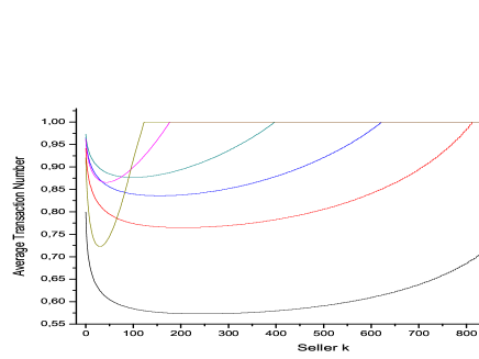
Figure 2: Average Number of Transactions as a function of quality $k$.

The average valuation ratio $\left\langle\gamma\left(k\right)\right\rangle$ (Fig. 3), in the symmetric information case, increase monotonically with the increasing of quality. By introducing asymmetry in the information low quality goods become more profitable. In other words, as $\beta$ decreases to $\beta_{c}$ the valuation ratio invert completely its behavior. But it is in the quality mid-region $\left[k\sim 50,k\sim 800\right]$ that an interesting behavior emerges. A significant lower level of transactions appears, becoming larger as $\beta$ approaches its critical level $\beta_{c}$ (affecting more products during the transition), while the valley deepness appears to decrease from $\beta\approx 0.9$ to $\beta\approx 0.5$, and to increase from $\beta\approx 0.5$ until it reaches its maximum level at $\beta_{c}=0.32$, as one can see in Fig. 2.

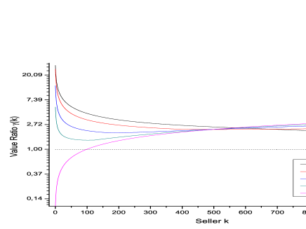
Figure 3: Value ratio $\gamma=V^{b}(k)/V^{s}(k)$, i.e. the gap between value given by buyer over the value due to the seller as a function of quality $k$.

The relative gain $\gamma\left(k\right)$ allows us to compare the relative firms’ profit as a function of the quality $k$ for several $\beta$ values. In the symmetric information case $\gamma$ is an increasing function, showing that it is more profitable to produce high quality goods.

Information asymmetry makes the low quality region become more profitable, which can be interpreted as an incentive for firms produce low quality goods. This is a consequence of the goods quality overestimation by buyers. We note that the minimum profit depends on $\beta$ and moves from low to high quality level, in particular, for $\beta=\beta_{c}$ the minimum $\gamma$ is the highest quality product.

It is important to note that when $\beta$ is close to $\beta_{c}$ it becomes difficult for buyer to recognize the real product quality . Below the critical point $\beta=\beta_{c}$ the buyers move away from the market because they become unable to distinguish the goods’ quality. This is the reason pointed out by Arkelof to explain the market failure, caused by information asymmetry associated with high variation in the quality of goods produced.

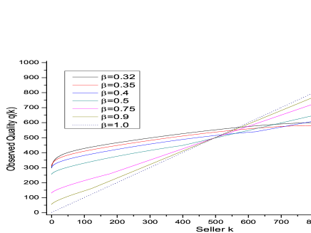
Figure 4: Observed quality $q$ as a function of quality $k$.

The general model overview is that an environment of perfect and symmetric information enables consumers to purchase products which they think are fairly evaluated. When their perception $\beta$ decreases from $\beta=1.0$ to $\beta_{c}$, low quality goods are traded in the market less frequently than those with high quality. The effect of reducing the information level is the decrease in the average rate of transactions. For a high information asymmetry ($\beta\approx\beta_{c}$), less transactions take place, mostly concentrated on very low and very high quality level goods. When the firms’ quality decrease, the trade probability also decreases (see Fig. 2) and so does the average transaction rate. However, we see in the Fig. 1 that there is a peak in the distribution $\Pi\left(k\right)$ in the region $k\leq\lambda^{\frac{1}{1-\alpha}}$, which explains the increasing transaction rate in this region for $\beta\approx\beta_{c}$.

6 Conclusions

The simplicity of the model allowed us to solve it analytically using the Markovian chain approach. The existence of stationary solutions is a condition for the systems to avoid the collapse. The model can be split in three regimes, according to the value of technological level $\alpha$. The role of the technology is to increase productivity and to reduce cost. In particular, we focused the analyzes on high technological regime ($\alpha=\frac{1}{2}$) since the economy evolves toward increasing efficiency.

The role of the asymmetric information is to enhance the low quality market. We showed that the consumers overestimate the quality of goods below the medium quality level. Thus the relative profit increases in the region of low quality, and a higher asymmetric information will imply higher profits in the production of the low quality goods. However, there is a critical asymmetric level above which the market collapses. This is explained as the breakdown of ergodicity, i.e., the asymmetry is so high that all those that buy low quality goods fall down in a trap and stop to trade. From the consumers’ viewpoint, the incapacity to distinguish high and low quality makes the agent leave the market.

From the seller’ point of view, it is hard to decide which quality would maximize her profit. It is necessary to know the value of several parameters from the market. This is not the mission of economics. In general Economics provides a theory that explains what will happen given the market set up. The design of strategies is the business of marketing science. The importance of general models is provide tools that help us to address this issue.

References

- [1] Akerlof G A 1970 Quart. J. of Econ. 84(3) 488-500.
- [2] Wang Y, Li Y and Liu M 2007 Phys. A 373 665.
- [3] Chau K W, Yiu C Y and Wong S K submitted for publication.
- [4] Zhang Y-C 2005 Phys. A 350 500.
- [5] Porter M E 1979 Harv. Bus. Rev. Mar-Apr 91-101.
- [6] Smith A 1776 An inquiry into the nature and causes of the wealth of nations B1.
- [7] Soberman D 2005 Mark. Science 24(1) 165-74.
- [8] Liu L, Medo M, Zhang Y-C and Challet D 2008 Eur. Phys. J. B 64 293.