Nonparametric Covariate Adjustment for Receiver Operating Characteristic Curves
Abstract
The accuracy of a diagnostic test is typically characterised using the receiver operating characteristic (ROC) curve. Summarising indexes such as the area under the ROC curve (AUC) are used to compare different tests as well as to measure the difference between two populations. Often additional information is available on some of the covariates which are known to influence the accuracy of such measures. We propose nonparametric methods for covariate adjustment of the AUC. Models with normal errors and non-normal errors are discussed and analysed separately. Nonparametric regression is used for estimating mean and variance functions in both scenarios. In the general noise case we propose a covariate-adjusted Mann-Whitney estimator for AUC estimation which effectively uses available data to construct working samples at any covariate value of interest and is computationally efficient for implementation. This provides a generalisation of the Mann-Whitney approach for comparing two populations by taking covariate effects into account. We derive asymptotic properties for the AUC estimators in both settings, including asymptotic normality, optimal strong uniform convergence rates and MSE consistency. The usefulness of the proposed methods is demonstrated through simulated and real data examples.
Keywords: Area Under Curve, Asymptotics, Covariate Adjustment, Mann-Whitney, Nonparametric, Smoothing, Uniform Convergence
1 Introduction
The receiver operating characteristic (ROC) curve is a commonly used tool for summarizing the accuracy of a test with binary results. The sensitivity, or true positive rate, of a binary test is the probability that a truly diseased subject is diagnosed as diseased. The specificity, which is also equal to one minus false positive rate, is defined as the probability that a healthy subject produces a negative test. Suppose that the result of a test is a random variable ; depending on whether or the test result is considered negative or positive, respectively. If the distribution of is continuous, each value of the threshold will correspond to different sensitivity and specificity values. In general the ROC curve summarizes how well two populations can be separated by a specified variable. Frequently a number of tests (a.k.a. markers or classifiers) are performed on each individual subject. A global univariate summary of the corresponding ROC curve is used to determine which classifier is more accurate. A number of such summaries are available but the most commonly used one is the area under the ROC curve (AUC). The AUC can be interpreted as the probability that a randomly chosen diseased subject will have a marker value greater than that of a randomly chosen nondiseased subject and can be used as an alternative measure of difference between two populations (e.g. Zhou et al., 2002). Its range of application extends from medical applications to reliability theory (Reiser and Guttman, 1986).
The presence of ROC curves has become ubiquitous in medical studies (Metz, 1989; Hsiao et al., 1989; Aoki et al., 1997; Otto et al., 1998; Stover et al, 1996; Zhou et al., 2002), its usage being spurred by the now classic text of Swets and Pickett (1982). Parametric and nonparametric methods for estimating individual ROC curves are available as well as methods that do not assume independent observations (Begg, 1991; Delong et al., 1988; Molodianovitch et al., 2006; Pepe, 2003).
In a large number of situations, additional information is available in the form of covariates which are known to influence the accuracy of the test. Only recently, statistical methods have been devised to incorporate such information in the ROC-based analysis. Some of the earlier methods have been produced by Thompson and Zucchini (1989), Obuchowski (1995), Tosteson and Begg (1988) and Toledano and Gatsonis (1995). Pepe (1997) formulated a general regression framework to model the dependence of the ROC curve directly on the covariates. Pepe (2000) and Dodd and Pepe (2003) propose semiparametric approaches to model the ROC and AUC directly using generalized linear models. Cai and Pepe (2002) extend the parametric ROC regression model by allowing an arbitrary nonparametric baseline function. Cai (2004) finds a more efficient estimator in the semiparametric setting. Brumback et al. (2006) used an alternative procedure by applying a generalized regression framework directly to the AUC in order to adjust the Mann-Whitney test for covariates. However, this approach loses the connection with the threshold value, does not allow the prediction of the sensitivity and specificity at a given threshold conditional on covariates nor does it model covariate effects on the individual marker values. Consequently we prefer to directly model the covariate effects on the marker values and through this modeling process obtain the analyses of interest.
The methods proposed in this paper fall within the first category of methods described in Pepe (1998). We propose a nonparametric approach to adjust for covariates the computation of AUC and other ROC-related quantities of interest. The main motivation for our method is the robustness to model mis-specification which may beset a parametric adjustment. We thus generalize in two ways the approaches of Faraggi (2003) and Schisterman et al. (2006) who use normal regression models to adjust the index AUC for covariates. We describe the regression model, distinguishing between the normal noise assumption and the general noise assumption. In a first extension of previous work, we estimate the mean and variance functions using nonparametric regression techniques, more specifically, local polynomial regression instead of parametric linear models. Our main contribution leading to the second extension is to construct a covariate-adjusted Mann-Whitney estimator (CAMWE) in the general noise case, which relies on working samples created at any possible covariate value of interest for the estimation of AUC. Such working samples have, for any , the same size as the original sample and can be used to estimate a number of covariate-adjusted characteristics of the ROC curve. In practice the computation is kept minimal by utilizing the estimated mean and variance functions for all of interest. We recommend bootstrapping in order to obtain confidence intervals for the covariate-adjusted AUC. Although we focus on covariate-adjusted AUC estimation, the proposed methods can be readily extended to other measures related to ROC curves, e.g., the covariate-adjusted specificity, sensitivity and Youden Index (Youden, 1950).
A theoretical investigation provides asymptotic results for both the normal noise and general noise models. The asymptotic normality and optimal strong uniform convergence rates for the covariate-adjusted AUC estimators for normal noise are established. For the general noise distribution we first derive asymptotic normality of the “hypothetical” CAMWE and then characterize the asymptotic behavior of the Mean Squared Error (MSE) of the CAWME. We performed simulations under a number of scenarios to demonstrate the effectiveness and robustness of the proposed estimators as well as the validity of the Bootstrap scheme for confidence band construction.
2 Model and Estimation
2.1 Regression Model
To motivate our proposal, we first note that parametric methods are used mainly for simple interpretation but may mis-specify the correct model forms, while nonparametric models provide an alternative solution and are more robust and data-adaptive. We attempt to achieve the robustness from two perspectives. First, we do not assume any parametric forms for the mean and variance functions of the test response variables, for nondiseased individuals and for diseased individuals. Although we refer to “diseased” and “nondiseased” groups, the above framework applies to any two populations of interest. We utilize nonparametric regression models
| (1) |
| (2) |
where denotes the covariate, the standardized errors and are independent of each other with zero mean and unit variance, and the variance functions and for all . Note that the errors here can depend heteroscedastically on the covariate through and . Second, we do not assume specific distributions for the noises in order to guard against mis-speciffication of error distributions. Denote the conditional cumulative distribution functions (c.d.f.) of and given by and , and c.d.f.s of and by and . Here we assume and do not depend on , i.e., the dependence of and on are expressed only through , , and , which is equivalent to a location-scale model. It is worth mentioning that, if the response variable is appropriately chosen at , then marker values of the diseased sample should be greater than that of the nondiseased sample on average. This is equivalent to , an assumption implicitly made for the remaining of the paper. If the baseline distributions and are symmetric about , it implies the assumption . In practice, we can simply constrain all the AUC estimators to be greater than 0.5. This would not affect any subsequent development due to the consistency of the unrestricted estimators as presented in Section 3. For notational convenience, we use the unrestricted forms throughout the paper.
This extends the first type of models discussed by Pepe (1998), where linear forms were assumed for and with variances not depending on the covariate , i.e., , , and . It is also noticed that we do not require the same baseline distributions of the standardized error and in contrast to Pepe (1998). Moreover, when the noise is not normally distributed, we shall propose a new estimator for the area under the ROC curve that extends the Mann-Whitney estimator for covariate-adjustment by using standardized residuals via the so-called working samples.
2.2 Estimation under Normal Noise Assumption
Let be the area under the ROC curve with the covariate adjustment . From models (1) and (2), when the errors and are normally distributed, i.e., , where is the c.d.f. of the standard normal, it is straightforward to derive the following explicit expression:
| (3) |
where the subscript “N” stands for the normal assumption. One can also obtain closed forms of the sensitivity and specificity for ,
| (4) |
for a given threshold . The ROC curve for the covariate is the plot of versus for all possible values of , and this can be explicitly written as
| (5) |
The unknown functions , are estimated by using nonparametric regression methods as addressed in Section 3.1, providing a “nonparametric adjustment” as discussed in Section 1.
2.3 Estimation under General Noise Assumption
The assumption of normal noise above simplifies the calculations of the AUC via (3) but is not always supported by the data. In addition, the normality assumption hampers the full generality one expects from a nonparametric model. We propose here a fully nonparametric yet simple estimator of the AUC with covariate adjustment, , for a general noise distribution.
The proposed estimator is motivated by the classical Mann-Whitney statistic, which is formulated for two samples and as
| (6) |
where if and otherwise. The data obtained from nondiseased and diseased samples consist of and , where is the observed covariate value in the nondiseased sample and in the diseased sample. It should be noticed that the markers and are evaluated at possibly different values of the covariate , and we are often interested in estimating even for z-values which were not measured in either group or both. To estimate at , one possibility is to include the marker values and that fall into neighborhoods of with appropriate weight functions. This consideration naturally leads to a bivariate kernel estimator that is fully nonparametric,
| (7) |
where and are bandwidths, when is a symmetric kernel density. However, , does not efficiently use the available data due to the restriction on the local windows, nor do the regression models (1) and (2) play any role here. Note that is obtained by smoothing the binary variables corresponding to covariate observations that are not necessarily located on the diagonal (in fact, and may have no overlap). It is unclear how to choose the bandwidths and which are critical to the kernel regression estimation, as the standard cross-validation procedure does not apply due to the absence of the observed on the diagonal of the bivariate covariate surface. More discussion and comparisons concerning will be presented in simulations in Section 4.
Based on the above considerations, we propose a different nonparametric estimator of which utilizes the entire collection of data available and the regression models (1) and (2). First, suppose that we can observe all the standardized residuals, , ,
| (8) |
Recall that the distributions of and do not depend on , implying that are independently and identically distributed (i.i.d.) with the c.d.f. for , and are i.i.d. with the c.d.f. for . In Pepe (1998) these standardized residuals can be used to obtain the empirical distributions of and . In a similar sprit, we propose a different way to utilize these residuals to construct working samples and as if they were all observed at ,
| (9) |
Then it is intuitive to use the proposed Covariate-Adjusted Mann-Whitney Estimator (CAMWE) for ,
| (10) |
This is a natural extension of the Mann-Whitney estimator since in the case of no covariate effect , , , are constant in and (10) becomes the traditional Mann-Whitney statistic. For practical implementation, after obtaining nonparametric estimates of and , we do not have to choose other tuning parameters for each covariate value , while (7) requires retuning. Analogously we can calculate the sensitivity and specificity from the working samples for ,
| (11) |
for a given threshold . The ROC curves for can be obtained by plotting versus for all possible values of .
Remark 1. Note that the central idea is to construct the working sample and for each . The entire conditional ROC curve, given the covariate value , can be obtained from (11). One can estimate any index of interest at using this working sample. For instance, the Youden Index (YI) (Youden, 1950) can be calculated by , where and are defined by (11), and its optimal threshold given can be found via a numerical search.
Remark 2. In principle, the proposed approach can be extended to the case of multiple covariates using different strategies. A natural consideration is to use multivariate nonparametric smoothing techniques that require extensive computation. An alternative is to use additive frameworks for mean and variance structures respectively, then construct the working sample in a similar spirit for each set of covariate values of interest.
2.4 Implementation via Nonparametric Regression
We exploit the local polynomial regression models for estimating the functions and . Let be a compactly-supported symmetric kernel density function with a finite variance, a sequence of bandwidths used to estimate , and a sequence of bandwidths for . Let be the order of local polynomial fit, e.g., and correspond to local constant and local linear fits, respectively. An odd order fit is often suggested (Fan and Gijbels, 1996) for both theoretical and practical considerations. In particular, for estimating the regression function itself, a common choice is the local linear fit with . Denote the resulting th order local polynomial estimators of and by and . Next, the variance functions and for heteroscedastic errors are estimated by fitting local polynomial regression to the squared residuals, and , ,
| (12) |
with bandwidths and . The detailed formulas of the aforementioned local polynomial estimators are given in Appendix 1. In the case of homoscedastic errors, and , it is easy to obtain root-n consistent estimators (Hall and Marron, 1990; Hall et al., 1990). The theoretical properties in Section 4 are still valid with slight modifications. In practice, the bandwidths , , and are chosen by the standard technique of leave-one-out cross-validation for estimating the mean and variance functions, while other existing techniques can certainly be applied. Such bandwidths usually fulfill the assumptions needed for theoretical developments in Section 3 for sufficiently large sample sizes. Substituting the local polynomial estimators , , and for these unknown quantities in formulae (3)-(5), (10) and (11) provides the point estimators , , , and for covariate .
To evaluate confidence limits and variances for AUC under normal noise, the existing formulation (Guttman et al., 1988; Faraggi, 2000, among others) are no longer valid due to nonparametric regression. In principle we can derive the approximate variance for AUC under normal noise, based on the asymptotic normality of the local polynomial estimators (Fan and Gijbels, 1996) using the Cramér-Wold device. However, due to the complicated asymptotic expressions with unknown functionals and their derivatives, the evaluation of such asymptotic quantities will require extensive pilot smoothing and further approximations. This might deteriorate the accuracy and not be worth further pursuing. Thus we choose to obtain confidence limits and variance estimates for AUC via “bootstrapping the original data” as proposed by Efron and Tibshirani (1993). We do not repeat the procedure here for conciseness. While this approach can be justified in normal noise case due to the limiting distributions in Theorem 1, it may not be the case under the general noise for which the asymptotic normality of the CAMWE is unknown at this moment. Nevertheless, the simulation performed in Section 4.1 offers empirical support to this bootstrap procedure for the general noise case.
Remark. Jointly choosing four bandwidths simultaneously aiming at the AUC estimator is prohibitively expensive, even impossible with available computing resources. Even if the computation load were not an issue, we would have no suitable criterion to perform the joint optimization for two reasons. First, if one bases the criterion on asymptotic bias and variance, these quantities involve unknown functionals and their derivatives and are too complicated for practical use. It should also be noticed that such asymptotic expressions are established only for the normal noise case. Second, if one attempts cross-validation directly for , there are no observed values of AUC at available, which is a similar issue as the one discussed for in Section 2.3.
3 Theoretical Properties
In this section we present the asymptotic theory developed for the nonparametric estimators of the AUC with covariate adjustment for under both normal and general noise assumptions. One can easily extend these arguments to obtain the corresponding asymptotic theory for the sensitivity and specificity with a given threshold value . These are not presented here for conciseness.
3.1 Asymptotic Properties under Normal Noise
We begin with the asymptotic normality of the estimated AUC under the normal noise assumption, where the target is exactly , i.e., . Let be the density function of the covariate that is treated as a random variable. Denote by a neighborhood of . Assume that, for a given value of ,
-
(A1)
and is continuous in .
Put , , and . Assume that, for a given ,
-
(A2)
, and are continuous in .
Recall that , , and are the sequences of bandwidths for estimating , , and . One can see that, if the bandwidths and are chosen optimally for estimating and , then and will be of the same order in terms of the sample size . Thus we assume the following, as ,
-
(A3)
, , for some , for some .
Analogously, for the estimation of and , we assume that, for a given ,
-
(A4)
, and are continuous in ;
-
(A5)
, , for some , and for some .
Here we consider the odd order of local polynomial estimators for , , and as argued in Section 2.4. The same order is used mainly for notational convenience, while we certainly can choose different orders in practice. With slight modifications, the results can be easily adapted to possibly different orders as well as the case of even . For the symmetric kernel density we assume that the j-th moment exists for all integer .
-
(A6)
, .
For convenience, we introduce the notion of the order of a kernel function. We say is an th order kernel function, provided that , for and . It is obvious that is a 2nd order kernel. Let the matrix , be the vector with the th element equal to 1 and 0 elsewhere, and
| (13) |
which is often referred to as the equivalent kernel. One can verify that is a th order kernel when is odd. Also denote for any .
Lemma 1 in Appendix 2 provides the joint asymptotic distributions of the local polynomial estimators of and , which is the basis for deriving the asymptotic distributions of . The difficulty in the proof of Lemma 1 is to deal with the dependence between the mean and variance estimators, while and are independent, see Appendix 2 for details. Based on Lemma 1, we exploit the Cramér-Wold device to obtain the asymptotic distribution of as follows.
Theorem 1
Under the assumptions (A1)-(A6) for a given ,
-
•
if , , where , ,
-
•
if , , where
-
•
if for some , , where
(16)
Besides the pointwise limiting distributions, we also establish the optimal rates for strong uniform convergence of in Theorem 2. Denote by the set of possible values of (usually an interval on the real line). Additional assumptions below are needed for the uniform convergence results,
-
(A7.1)
for some , where is the joint density of .
-
(A7.2)
for some , where is the joint density of .
For the proof of Theorem 2 we need to modify (A1)-(A6) as follows. For convenience we impose conditions on the equivalent kernel (13) instead of the original kernel .
-
(A1†)
, and is bounded and continuous on .
-
(A2†)
On the domain , for some and is bounded, is bounded, , , and are bounded and continuous.
-
(A3†)
for some , for some , where satisfies (A7.1).
-
(A4†)
On the domain , for some and is bounded, is bounded, , , and are bounded and continuous.
-
(A5†)
for some , for some , where satisfies (A7.2).
-
(A6†)
is uniform continuous, absolutely integrable with respect to Lebesgue measure on and of bounded variation, as , .
Lemma 2 in Appendix 2 presents the strong uniform convergence rates of the local polynomial estimators of the mean and variance functions. Then the strong uniform convergence rate of is obtained immediately below, where a.s. is the abbreviation of “almost surely”.
Theorem 2
Under the assumptions (A1†)-(A6†), (A7.1) and (A7.2), let and , then
| (17) |
3.2 Asymptotic Properties under General Noise
Now we turn to the asymptotic properties of the CAMWE of under the general noise assumption. We first state the asymptotic normality of the “hypothetical” estimator (10) that contains true values of the unknown mean and variance functions, while our target is . Recall that and are the c.d.f.s of standardized errors and , and do not depend on the covariate . Define
Set and .
Theorem 3
In the next theorem we establish the MSE consistency of the CAMWE for the “hypothetical” estimator for a given covariate , based on uniform consistency of the estimated mean and variance functions. It is noticed in the proof that we actually do not need the optimal strong uniform convergence rates stated in Lemma 2, as these rates cannot be passed to , while uniform consistency in probability is sufficient. Thus the regularity conditions (A3†) and (A5†) can be relaxed to the following.
-
(A3∗)
, for some , where satisfies (A7.1).
-
(A5∗)
, for some , where satisfies (A7.2).
We also need the following additional assumptions,
-
(A8)
and are continuous on their domains.
Theorem 4
Under (A8) and the assumptions for Theorem 2 with (A3) and (A5) replaced by (A3∗) and (A5∗), for a given ,
| (20) |
We conclude this section with the following corollary that is a direct consequence of Theorem 3 and 4. Note that the MSE discrepancy between estimated and true AUC at is dominated by the nonparametric rate in (20) that is usually slower the the parametric rate , although its order of magnitude is not obtainable, at least to our knowledge.
Corollary 1
Under (A8) and the assumptions for Theorem 2 with (A3) and (A5) replaced by (A3∗) and (A5∗), for a given ,
| (21) |
4 Simulations and Data Example
4.1 Simulations
The purpose of the simulations is to assess the performance of the methods for estimating AUC in nonparametric regression settings. We have not compared our method with parametric models since the two approaches address different situations. If a parametric model is correctly specified, its performance will be superior to a nonparametric procedure; however, if there is no known parametric model suitable for the data considered, one will have no choice but to use the nonparametric tools available.
We consider three situations for illustration. In the first situation the underlying models are, for non-diseased and diseased individuals respectively,
| (22) |
where the errors and are standard normal, the conditional variance functions are and , , . The covariates and are independently generated from , and moderate sample sizes are used. The identical setting is used in the second situation, except that the errors and are generated from a Student- distribution with 3 degrees of freedom and rescaled to have zero mean and unit variance.
The third situation, in which the log-transformed responses have normal errors and , i.e., the responses are generated from log-normal models, is designed to demonstrate the robustness of the proposed CAMWE . Since a log-transform often stabilizes the variability, we assume a constant variance on log-scale for both groups. Let and be the mean functions on log-scale, while and correspond to the original scale. From the properties of the log-normal distribution, one has
We choose and , , and . Then the models are completely determined and can be written as
| (23) |
where the covariates and are independently generated from , and are standard normal errors, , .
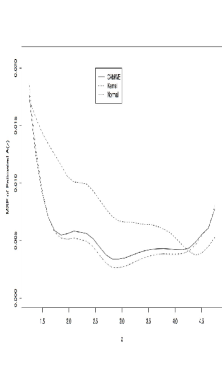
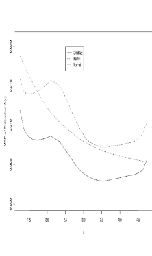
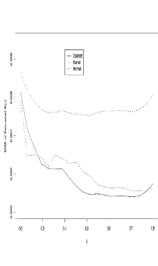
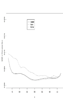
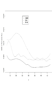
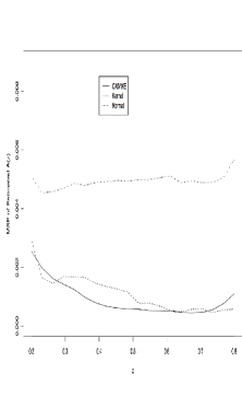
With the generated data we compared three estimators, with normal noise assumption, CAMWE with general noise assumption as well as the kernel estimator . For bandwidth choices, recall that joint selection aiming for and is not feasible and that cross-validation fails for . To make the comparisons possible, for and we minimized the true integrated squared errors respectively, say to select , and similarly for , and , while was minimized for choosing and in . One can see that, if one targets at , the bandwidths chosen for and may not be as “optimal” as those for . However, it is demonstrated below that even in such a disadvantageous situation, the proposed estimators, especially , are still preferable. We used the sample sizes of and , while all the estimates were improved with increased sample sizes as expected. All three AUC estimates are obtained by applying the estimation procedures to the simulated data and (on original scale throughout) in the aforementioned three situations. Monte Carlo averages (calculated from 500 runs in each case) of Mean Squared Errors at different values of are presented in Figure 1. We can see that, for the normal noise model the CAMWE and normal estimator are comparable and both outperform the kernel estimator . Although improves upon under the heavy-tailed Student- noise model, the CAMWE is still the most effective. For the log-normal model, when we apply these three estimation procedures to the original responses, the CAMWE and kernel estimators yield comparable results (CAMWE seems slightly better), and both significantly improved upon the normal estimator.
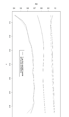
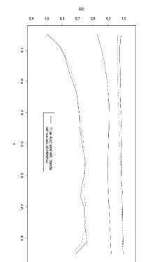
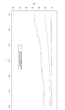
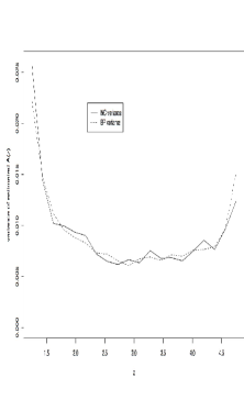
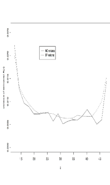
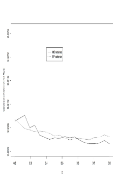
Now we examine the empirical performance of the pointwise confidence bands and variance estimates obtained by “bootstrapping the data” in the general noise case, i.e. when the CAMWE is used for estimation, we carried out an additional study. We used the same settings for the three models with normal, Student with 3 degrees of freedom and log-normal noises, respectively. The benchmark used for comparison is the 95% pointwise confidence bands and variance estimates averaged from 500 Monte Carlo runs. In each Monte Carlo run, was obtained and we bootstraped the data 1000 times to calculate 95% bootstrap bands (defined between the 2.5th and the 97.5th percentiles) and bootstrap sample variance. All the bandwidths involved in the estimation are selected respectively by leave-one-out cross-validation in smoothing steps. In the top panels of Figure 2 we reported, for all three data-generating models with moderate sample sizes , the comparisons between the Monte Carlo averages of the bootstrap bands and the Monte Carlo bands. In the bottom panels, similar comparisons were shown for the averaged bootstrap variance estimates of against the Monte Carlo variances. From Figure 2, for the CAMWE , the averages of confidence bands obtained by “bootstrapping the data” approximate well the 95% pointwise Monte Carlo bands. The same can be said about the averages of bootstrap variance estimates. This provides some empirical evidence for using the bootstrap confidence bands and variance estimates for the CAMWE in the general noise case. For the normal noise model, we have done similar comparisons and the results are almost identical to those obtained for (thus not reported for brevity).
4.2 Real Data Example
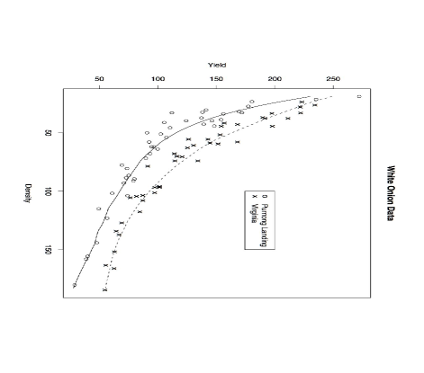
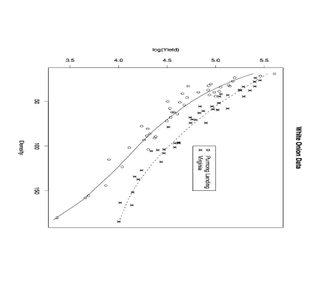
We consider the white onions data originally reported by Ratkowski (1983) on the density-yield relationship of varieties of white Spanish Onion grown in various regions of Australia. The data has been the subject of a nonparametric analysis of covariance in Young and Bowman (1995). One can see from Figure 3 that the relationship between the density and yield is non-linear for the two regions considered here: Virginia and Purnong Landing. A question of interest is whether the two regions of origin for the onions can be separated simply by looking at the yield. Figure 3 shows that the difference between yields depends on the density which will be the covariate under consideration in our study.
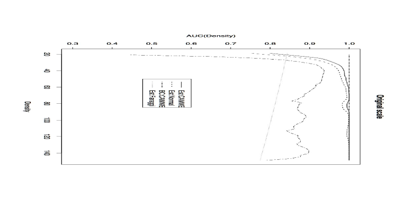
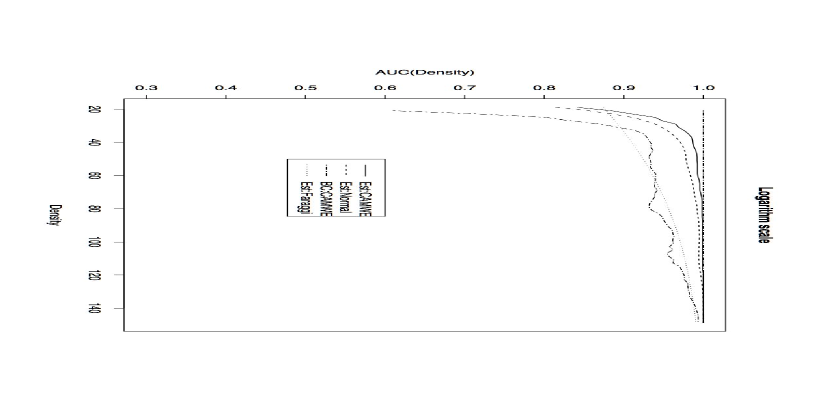
If we apply directly the method of Faraggi (2003) to the data on the original scale we observe a large discrepancy between the parametric and nonparametric analyses, as illustrated by the top panel in Figure 4. We also notice that bootstraping the data produces wider 95% confidence bands for large values of the density due to the sparseness and high variability. But even such confidence bands do not cover the parametric estimators of the AUC. We should note that due to the sparseness of observations with densities larger than 150 we focus on the covariate range . On the logarithmic scale, the relationship between yield and density is more linear as can be seen from the bottom panel in Figure 3. In addition, the transformation seems to stabilize the variance so it is not unexpected that he difference between the nonparametric approach and the parametric one diminishes. We can also notice that, on both original and logarithmic scales, the estimates obtained under the normal assumption are more conservative indicating a smaller AUC for small densities. This indicates that the normal assumptions may not be valid for this dataset and that the nonparametric approach is more suitable due to its robustness.
5 Conclusions
We introduce nonparametric adjustment for covariate information in the context of ROC analysis, more specifically for the AUC index. The essential idea in our proposal is that the conditional ROC curve and all the indexes associated with it (e.g. Youden Index (YI) and its optimal cutoff value) can be computed using the statistical model and, subsequently, the reconstructed working sample. The theoretical properties of the index estimators deserve further investigation. The approach bears some similarity to the work on nonparametric adjustment for covariates when estimating a treatment effect as in Young and Bowman (1995) and Cantoni and de Luna (2006) and advances in that field are likely to yield newer results for the ROC covariate adjustment. In contrast to their work we focus on a generalized Mann-Whitney approach. Our simulations demonstrate effectiveness and robustness of the proposed method. While the discussion is limited to the case of only one covariate, the proposed approach can be extended to multiple covariates in various ways (e.g.,̇ additive models). It is expected that the computational load will significantly increase with each additional covariate added to the model. In principle one may consider reasonable parametric approximations suggested by nonparametric approaches that lead to simpler interpretations. For instance, one possibility is to use parametric models for the mean and variance functions following the nonparametrically estimated forms. Similar strategy applies to approximating the empirical c.d.f. of the noise by parametric functions.
Appendix 1: Local Polynomial Estimators
Recall that and are nondiseased and diseased samples. The local polynomial regression estimator of is obtained by minimizing
| (24) |
where is the bandwidth controlling the amount of smoothing, and . It is more convenient to work with matrix notation. Denote the design matrix of (24) by ,
and put and . The local polynomial estimator is then given by
| (26) |
Analogously for the diseased sample , the design matrix and weight matrix are similarly defined, letting , then the local polynomial estimator for is
We next estimate the variance functions and for heteroscedastic errors according to models (1) and (2). The nonparametric estimators and are obtained by fitting local polynomial regression to the squared residuals, i.e., the variance observations and as in (12). Let and be the sequences of bandwidths for and . Denote and , we have
where and are defined as the above, and .
Appendix 2: Auxiliary Results and Proofs
Lemma 1
If the assumptions (A1)-(A3), (A6) hold, and , for a given ,
| (27) |
where and with
Analogously, if the assumptions (A1), (A4)-(A6) hold, and , for a given ,
| (28) |
where and with
Proof of Lemma 1. The asymptotic normality of with the bias and the variance is standard in local polynomial regression. Let , note that the input data . Applying a local polynomial fit to , one can see that the second term will result in a quantity of the order and the third term will yield . It is obvious that both quantities are ignorable, compared to the local polynomial estimator obtained by fitting . Therefore the estimators and are asymptotically equivalent with the same limit distribution. Again we apply the standard argument of local polynomial regression to obtain the asymptotic normality of with the bias and variance . To derive the covariance of the limit distribution between and , one can equivalently work with and . Using the equivalent kernel notation , the limiting covariance is identical to the following, obtained by employing a Taylor expansion,
where
The same arguments can be applied to obtain the joint asymptotic distribution in (28).
Proof of Theorem 1. The Cramér-Wold device is exploited to derive the asymptotic distributions of for three possible cases, and the detailed proof is omitted for conciseness.
Lemma 2
If the assumptions (A1†)-(A3†), (A6†) and (A7.1) hold, and ,
| (29) |
and If the assumptions (A1†), (A4†)-(A6†) and (A7.2) hold, and ,
| (30) |
where and as defined in Theorem 2.
Proof of Lemma 2. It is sufficient to show (29). The strong uniform convergence rate for was obtained by Horng (2006), which is based on the arguments in Silverman (1978) and Mack and Silverman (1982) and the equivalent kernel representation, we follow the similar argument used in the proof of Lemma 1. Recall that , and . Applying a local polynomial fit to , , the second and third terms of the resulting estimator tend to 0 with probability 1, and the leading term has the strong uniform convergence rate by using the same argument for .
Proof of Theorem 2. The proof follows Lemma 2 and the uniform version of Slutsky’s Theorem. It is only needed to note that, if (A2†) and (A4†) hold, has bounded partial derivative in each argument, and thus satisfies Lipschitz continuity.
Proof of Theorem 3. For a given , one can see that “hypothetical” estimator is in fact a two-sample U-statistic. The argument used in the theory of U-statistics can be applied here. The unbiasedness of is obvious. For the asymptotic variance at a given , put , . , . Note that
and similarly , i.e., , as specified in Theorem 3. The unbiasedness of is obvious from . For the variance calculation, after some counting techniques, one has,
| (31) |
where is the combination of choosing from . This proves (18).
To show the asymptotic normality (19), define
which is in fact the projection of on the space formed by random variables of the form of , where and are arbitrary measurable functions. From Hájek’s Projection Theorem and (31), we have, as ,
which, together with unbiasedness, implies that is asymptotically equivalent to . Then following central limit theorem, when and , has the limiting distribution as specified in (19). So does .
Proof of Theorem 4. Define and , and the dependences of and on and are suppressed for simplicity. Let , , , , , and then
where “” is the generic notation for estimated quantities. By analogy to the proof of Lemma 2 with the assumptions (A3†) and (A5†) replaced by (A3∗) and (A5∗), we obtain weak (in probability) uniform consistency of , , and . This is sufficient for our purpose, the reason of which will be singled out below. Again by analogy to the proof of Theorem 2 with the uniform version of Slutsky’s Theorem (in probability instead of almost sure), we have, for a given , , , , for and . Since , one has and, analogously, , regardless of and . Also note that , , and are bounded on , then we obtain that only depends on the given .
To show (20), we observe that , where
while , and are defined in the same way, with corresponds to , to and to . We first focus on ,
| (32) | |||||
For any given , from Slutsky’s Theorem, we have , and converge in probability to uniformly in all arguments except , which implies uniform convergence in distribution. Therefore the four sequences of probabilities in (32) all uniformly converge to as , which leads to . From the above argument, one can see that the weak uniform consistency is sufficient, also that the convergence rates cannot be preserved for evaluating upper bounds for those probability differences. Using similar arguments, it is easy to show that , and . This completes the proof of Theorem 4.
References
- Aoki et al. (1997) Aoki, K., J. Misumi, T. Kimura, W. Zhao, and T. Xie (1997). Evaluation of cutoff levels for screening of gastric cancer using serum pepsinogens and distributions of levels of serum pepsinogens I, II and of PG I/PG II ratios in a gastric cancer case-control study. Journal of Epidemiology 7, 143–151.
- Begg (1991) Begg, C. B. (1991). Advances in statistical methodology for diagnostic medicine in the 1980’s. Statistics in Medicine 10, 1887–1895.
- Brumback et al. (2006) Brumback, L. C., M. S. Pepe, and T. A. Alonzo (2006). Using the ROC curve for gauging treatment effect in clinical trials. Statistics in Medicine 25, 575–590.
- Cai (2004) Cai, T. (2004). Semi-parametric ROC regression analysis with placement values. Biostatistics 5, 45–60.
- Cai and Pepe (2002) Cai, T. and M. Pepe (2002). Semiparametric receiver operating characteristic analysis to evaluate biomarkers for disease. Journal of the American Statistical Association 97, 1099–1107.
- Cantoni and de Luna (2006) Cantoni, E. and X. de Luna (2006). Non-parametric adjustment for covariates when estimating a treatment effect. Nonparam. Statist. 18, 227–244.
- Delong et al. (1988) Delong, E. R., D. M. Delong, and D. L. Clarke-Pearson (1988). Comparing the area under two or more correlated receiver operating characteristic curves: a nonparametric approach. Biometrics 44, 837–844.
- Dodd and Pepe (2003) Dodd, L. and M. Pepe (2003). Semi-parametric regression for the area under the Receiver Operating Characteristic Curve. J. Amer. Statist. Assoc. 98, 409–417.
- Efron and Tibshirani (1993) Efron, B. and R. J. Tibshirani (1993). An Introduction to the Bootstrap. New York: Chapman & Hall.
- Fan and Gijbels (1996) Fan, J. and I. Gijbels (1996). Local Polynomial Modelling and Its Applications. London: Chapman & Hall.
- Faraggi (2000) Faraggi, D. (2000). The effect of random measurement error on receiver operating characteristic (ROC) curves. Statist. Medicine 19, 61–70.
- Faraggi (2003) Faraggi, D. (2003). Adjusting receiver operating curves and related indices for covariates. The Statistician 52, 179–192.
- Guttman et al. (1988) Guttman, I., R. A. Johnson, G. K. Bhattacharyya, and B. Reiser (1988). Confidence limits for stress-strength models with explanatory variables. Technometrics 30, 161–168.
- Hall et al. (1990) Hall, P., J. W. Kay, and D. M. Titterington (1990). Asymptotically optimal difference-based estimation of variance in nonparametric regression. Biometrika 77, 521–528.
- Hall and Marron (1990) Hall, P. and J. S. Marron (1990). On variance estimation in nonparametric regression. Biometrika 77, 415–419.
- Horng (2006) Horng, W. J. (2006). Uniform consistency and convergence rate in the local polynomial estimation of regression. Journal of Science and Engineering Technology 2, 61–66.
- Hsiao et al. (1989) Hsiao, J. K., J. J. Barko, and W. Z. Potter (1989). Diagnosing diagnoses: receiver operating characteristics methods and psychiatry. Archives of General Psychiatry 46, 664–667.
- Mack and Silverman (1982) Mack, Y. P. and B. W. Silverman (1982). Weak and strong uniform consistency of kernel regression estimates. Z. Wahrscheinlichkeitstheorie and Verwandte Gebiete 61, 405–415.
- Molodianovitch et al. (2006) Molodianovitch, K., D. Faraggi, and B. Reiser (2006). Comparing the areas under two correlated ROC curves: Parametric and non-parametric approaches. Biometrical Journal 48, 745–757.
- Obuchowski (1995) Obuchowski, N. (1995). Multireader, multimodality receiver operating characteristic curve studies: Hypothesis testing and sample size estimation using an analysis of variance approach with dependent observations. Acad. Radiol. 2, 522–529.
- Otto et al. (1998) Otto, M., J. Wiltfang, E. Sch utz, A. Otto, A. Pfahlberg, O. Gefeller, M. Uhr, A. Giese, T. Weber, H. A. Kretzschmar, and S. Poser (1998). Diagnosis of creutzfeldt-jacob disease by measurement of s100 protein in serum: prospective case-control study. Br. Med. J. 316, 577–586.
- Pepe (1997) Pepe, M. S. (1997). A regression modelling framework for receiver operating characteristics curves in medical diagnostic testing. Biometrika 84, 595–608.
- Pepe (1998) Pepe, M. S. (1998). Three approaches to regression analysis of receiver operating characteristic curves for continuous test results. Biometrics 54, 124–135.
- Pepe (2000) Pepe, M. S. (2000). An interpretation for the ROC curve and inference using GLM procedures. Biometrics 56, 352–359.
- Pepe (2003) Pepe, M. S. (2003). The Statistical Evaluation of Medical Tests for Classification and Prediction. Oxford Statistical Sciences Series.
- Ratkowsky (1983) Ratkowsky, D. A. (1983). Nonlinear Regression Modelling (Statistics: Textbooks and Monographs, Volume 48). Marcel Dekker: New York.
- Reiser and Guttman (1986) Reiser, B. and I. Guttman (1986). Stastistical-inference for pr(y-less-than-x) - the normal case. Technometrics 28, 253–257.
- Schisterman et al. (2004) Schisterman, E., D. Faraggi, and B. Reiser (2004). Adjusting the generalized ROC curve for covariates. Statistics in Medicine 23, 3319–3331.
- Schisterman et al. (2006) Schisterman, E., B. Reiser, and D. Faraggi (2006). ROC analysis for markers with mass at zero. Statistics in Medicine 23, 623–638.
- Silverman (1978) Silverman, B. W. (1978). Weak and strong uniform consistency of the kernel estimate of a density and its derivatives. The Annals of Statistics 6, 177–184.
- Stover et al. (1996) Stover, L., M. Gorga, and S. Neely (1996). Toward optimizing the clinical utility of distortion product otoacoustic emission emission measurements. Journal of the Acoustical Society of America 100, 956–967.
- Swets and Pickett (1982) Swets, J. A. and R. M. Pickett (1982). Evaluation of Diagnostic Systems: Methods from Signal Detection Theory. Academic Press: New York.
- Thompson and Zucchini (1989) Thompson, M. L. and W. Zucchini (1989). On the statistical analysis of ROC curves. Statist. Med. 8, 1277–1290.
- Toledano and Gatsonis (1995) Toledano, A. and C. Gatsonis (1995). Regression analysis of correlated receiver operating characteristic data. Acad. Radiol. 2, 530–536.
- Tosteson and Begg (1988) Tosteson, A. N. A. and C. B. Begg (1988). A general regression methodology for ROC curve estimation. Med. Decision Mak. 8, 204–215.
- Youden (1950) Youden, W. J. (1950). Index for rating diagnostic tests. Cancer 3, 32–35.
- Young and Bowman (1995) Young, S. G. and A. W. Bowman (1995). Non-parametric analysis of covariance. Biometrics 51, 920–931.
- Zhou et al. (2002) Zhou, X. H., N. A. Obuchowski, and D. K. McClish (2002). Statistical Methods in Diagnostic Medicine. Wiley: New York.
