Loop Corrections to Cosmological Perturbations in Multi-field Inflationary Models

Xian Gao
Key Laboratory of Frontiers in Theoretical Physics,
Institute of Theoretical Physics, Chinese Academy of Sciences, Beijing 100190, P.R.China
E-mail
gaoxian@itp.ac.cn
   Fanrong Xu
Key Laboratory of Frontiers in Theoretical Physics,
Institute of Theoretical Physics, Chinese Academy of Sciences, Beijing 100190, P.R.China,
and
Maryland Center for Fundamental Physics and Department of Physics ,
University of Maryland, College Park, MD 20742, USA
E-mail
frxu@itp.ac.cn
Abstract:

We investigate one-loop quantum corrections to the power spectrum of adiabatic perturbation from entropy modes/adiabatic mode cross-interactions in multiple DBI inflationary models. We find that due to the non-canonical kinetic term in DBI models, the loop corrections are enhanced by slow-varying parameter ϵitalic-ϵ\epsilon and small sound speed cssubscript𝑐𝑠c_{s}. Thus, in general the loop-corrections in multi-DBI models can be large. Moreover, we find that the loop-corrections from adiabatic/entropy cross-interaction vertices are IR finite.

Cosmological perturbation theory, Inflation, Cosmology of theories beyond the SM, Physics of the early universe
preprint: CAS-KITPC/ITP-109

1 Introduction

Current observational data support standard ΛΛ\LambdaCDM model greatly [1], in which primordial perturbations which are assumed to be responsible for Cosmic Microwave Background anisotropies and large-scale structure formation are generated from quantum fluctuations and stretched to superhorizon scales during inflation (see e.g. [2] for a review). Standard single-field slow-roll inflationary models predict almost scale-invariant, Gaussian and adiabatic primordial fluctuation.

Actually, inflation itself is not a single model, but rather a theoretical framework. From the point of view of power spectrum, many inflation models are “degenerate”. Power spectrum, or strictly speaking, tree-level two-point correlation functions of cosmological perturbation do not give us an unique theory of inflation. In fact, phenomena beyond linear-order have been extensively investigated over the past several years.

The most significant progress beyond power spectrum is the investigation of statistical non-gaussianities of CMB anisotropies and primordial fluctuations (see e.g. [4] for a nice review). From the field theoretical point of view, non-gaussianity describes the interactions of perturbations, which will cause non-vanishing higher-order correlation functions. Such interactions are mandatory in any realistic inflationary models, which come from both the non-linear nature of gravity and the self-interactions of inflation field(s). In standard slow-roll inflation scenario, however, the non-gaussianities have been proved too small to be detected [3], even with PLANCK. Thus, any detection of non-gaussianties would not only rule out the simplest inflation models but also give us valuable insight of fundamental physics of inflation. Various models have been investigated to generate large non-gaussianties by introducing more complicated kinetic terms [5, 6, 7, 8] or more fields [9, 10, 11, 12, 13, 14, 15, 16, 18, 19, 22, 23].

Interactions not only cause non-vanishing higher-order correlation functions which are responsible for non-gaussianities of primordial perturbations, they also cause quantum loop-corrections. It is possible that such loop corrections may be large in their own right. Especially, we could expect large loop corrections in models which have also large non-gaussianties, since both of them describe the interactions among perturbations. Moreover, by collecting signatures of both quantum loop corrections and non-gaussianties, we will obtain a more sensitive test of the physics of inflation.

Early estimations of loop effects in cosmological perturbations were pioneered by Mukhanov, Abramo and Brandenberger [24, 25], Abramo and Woodard [26], and Unruh [27]. Subsequently, loop effects have been investigated by many authors [28, 29, 30, 31, 32, 33, 34, 35, 36, 37, 38, 39, 40, 41, 42, 43, 44, 45, 46, 47, 48, 49]. Recently, stimulated by works of S. Weinberg [50, 51], loop corrections to primordial fluctuations have been re-investigated by several authors [52, 53, 54, 55, 56, 57, 58, 59]. It has been found that cosmological loop corrections seem to have some infrared divergences, which scale as ln(k)𝑘\ln(k\ell), where 1superscript1\ell^{-1} is some IR comoving momentum cut-off [52, 53, 54, 55]. Other discussions on cosmological loop corrections and the infrared divergences can be found in [63, 64, 65, 66, 67, 68, 69]. The presence of IR divergences implies that loop-contributions may potentially give large corrections to tree-level results, although it was argued in [63, 64, 65] that these IR divergent corrections do not contribute in quantities that are directly observable.

Actually, now there are two types of so-called “loop corrections” in the literatures. One type is the quantum loops (q-loop) which originate from the interactions among fields and are evaluated using standard quantum field theory, while the other type is the classical loops (c-loop) which arise mathematically from some “loop-type integrals” due to the non-linear map from δϕ𝛿italic-ϕ\delta\phi to ζ𝜁\zeta [60, 61, 62]. In this work, we focus on the quantum loops. However, it is well-known that the observational variable is the curvature perturbation ζ𝜁\zeta and there has non-linear relation between ζ𝜁\zeta and δ𝛿\delta during superhorizon evolution (e.g. in terms of the “δN𝛿𝑁\delta N-formalism” [73, 74, 75]). Thus, these “loop” effects also have to be treated seriously ,and especially they can be significant, if the higher-order derivatives of e-folding number N with respect to the inflaton fields are extremely large. While in [62] it was shown that the loop corrections for ζ𝜁\zeta are always suppressed during inflation, if one assume that the fields follow a classical background trajectory.

Up to now, one-loop corrections to the power spectrum of the cosmological perturbations have been investigated in single scalar-field loops [52, 53, 54, 55, 50, 51], concerning effects from many light scalar fields [57], and from graviton loops [56]. Actually, it has been recognized that it is hard to generate large “local-type” non-gaussianities in single-field models, unless we abandon the slow-roll-type conditions. Thus, the investigation of multiple field models has particular importance. In multiple field inflationary models, perturbations can be decomposed instantaneously into one adiabatic mode and several entropy modes [20] (see [21] for a review). There are interactions between adiabatic mode and entropy modes.

In this work, we investigate the one-loop corrections to adiabatic power spectrum due to the interactions between entropy mode and adiabatic mode, at the horizon exiting. We find that due to the non-canonical kinetic term in DBI models, the loop corrections are enhanced by slow-varying parameter ϵitalic-ϵ\epsilon and small sound speed cssubscript𝑐𝑠c_{s}, as the enhancement of non-gaussianties in such models. Thus, in general, the loop-corrections in multi-DBI models can be large. Moreover, we find that the loop-corrections from adiabatic/entropy cross-interaction vertices are IR finite. This is because in the limit of speed sound cssubscript𝑐𝑠c_{s}, the leading-order three-point interactions are totally “derivatively interacted”. While the derivatives (both with respect to time and space) give momentum factors which cancel the momentum factors in the denominator from the tree-level correlation functions to make the loop-integrals IR safe.

Quantum cosmological correlation functions are evaluated by using “in-in formalism” (also dubbed as “Schwinger-Keldysh formalism” ) [70, 71, 72] (also see e.g. [50] for a nice review), which we also give a brief review in Appendix A. In [58] the application of “in-in” formalism on cosmological perturbation, especially on loop corrections, has been investigated in details.

This paper is organized as follows. In section 2, firstly we briefly review the linear perturbation of multiple-DBI models, then we describe the third-order perturbation action, especially the three-point adiabatic/entropy modes cross-interaction vertices. In section 3, we calculate the one-loop corrections to the adiabatic power spectrum from the adiabatic/entropy modes cross-interaction vertices, by using the “in-in” formalism. Finally, we make a conclusion and discuss the related issues.

In this paper, we set =c=8πG=1Planck-constant-over-2-pi𝑐8𝜋𝐺1\hbar=c=8\pi G=1.

2 Basic Setup

Perturbation theory of general multiple field modes with non-canonical kinetic terms up to third-order action has been calculated by several authors [10, 11, 12, 13, 14, 15, 16, 17, 22]. In this work, we focus on multi-field DBI models [10, 11, 12, 13, 14, 15, 16]. In this section, we briefly review previous known results and setup our conventions.

2.1 The model and the background

In this work, we focus on two-field DBI inflationary models, with action of the form

S=d4x(12R+ϕ),𝑆superscript𝑑4𝑥12𝑅superscriptitalic-ϕS=\int d^{4}x\,\left(\frac{1}{2}R+\mathcal{L}^{\phi}\right)\,, (1)

with111In general, the full DBI-type action takes the form =1f(D1)V1𝑓𝐷1𝑉\mathcal{L}=-\frac{1}{f}\left(\sqrt{D}-1\right)-V, with D=det(δIJ2fXIJ)12fX+4f2XI[IXJJ]8f3XI[IXJJXKK]+16f4XI[IXJJXKKXLL].D=\det\left(\delta_{IJ}-2fX_{IJ}\right)\equiv 1-2fX+4f^{2}X^{[I}_{I}X^{J]}_{J}-8f^{3}X^{[I}_{I}X^{J}_{J}X^{K]}_{K}+16f^{4}X^{[I}_{I}X^{J}_{J}X^{K}_{K}X^{L]}_{L}\,. However, it is shown that higher-order terms proportional to f3superscript𝑓3f^{3} and f4superscript𝑓4f^{4} do not contribute to the calculation of power spectra and leading order bispectra. Thus, in this work we neglect these terms for simplicity. One can refer [10, 11, 12, 13, 14, 15, 16] for detailed investigations of multi-DBI inflation models.

ϕ1f(ϕI)(12fX+2f2(X2XIJXIJ))V(ϕI),superscriptitalic-ϕ1𝑓superscriptitalic-ϕ𝐼12𝑓𝑋2superscript𝑓2superscript𝑋2subscript𝑋𝐼𝐽superscript𝑋𝐼𝐽𝑉superscriptitalic-ϕ𝐼\mathcal{L}^{\phi}\equiv-\frac{1}{\sqrt{f(\phi^{I})}}\left(\sqrt{1-2fX+2f^{2}\left(X^{2}-X_{IJ}X^{IJ}\right)}\right)-V(\phi^{I})\,, (2)

where

XIJ12μϕIμϕJ,superscript𝑋𝐼𝐽12subscript𝜇superscriptitalic-ϕ𝐼superscript𝜇superscriptitalic-ϕ𝐽X^{IJ}\equiv-\frac{1}{2}\partial_{\mu}\phi^{I}\partial^{\mu}\phi^{J}\,, (3)

and XGIJXIJ𝑋subscript𝐺𝐼𝐽superscript𝑋𝐼𝐽X\equiv G_{IJ}X^{IJ}.

The slow-rolling parameter is defined as usual

ϵ=H˙H2.italic-ϵ˙𝐻superscript𝐻2\epsilon=-\frac{\dot{H}}{H^{2}}\,. (4)

The background “inflaton velocity” σ˙˙𝜎\dot{\sigma} can be related with ϵitalic-ϵ\epsilon as

σ˙2X=H2ϵcs,˙𝜎2𝑋𝐻2italic-ϵsubscript𝑐𝑠{}\dot{\sigma}\equiv\sqrt{2X}=H\sqrt{2\epsilon c_{s}}\,, (5)

where cssubscript𝑐𝑠c_{s} plays the role of the propagating speed of the perturbation. In DBI inflation model,

cs212fX,superscriptsubscript𝑐𝑠212𝑓𝑋c_{s}^{2}\equiv 1-2fX\,, (6)

where X𝑋X is evaluated with the background quantities.

2.2 Brief review of linear perturbation

In multi-field inflation models, perturbations can be instantaneously decomposed into one adiabatic mode and several entropy modes [20]. Restricting to two-field case, we introduce the basis {eσ,es}subscript𝑒𝜎subscript𝑒𝑠\left\{e_{\sigma},e_{s}\right\} with eσIϕ˙I/σ˙superscriptsubscript𝑒𝜎𝐼superscript˙italic-ϕ𝐼˙𝜎e_{\sigma}^{I}\equiv\dot{\phi}^{I}/\dot{\sigma}, where σ˙˙𝜎\dot{\sigma} is the background inflaton velocity defined in (5), and esIsuperscriptsubscript𝑒𝑠𝐼e_{s}^{I} is orthogonal to eσIsubscriptsuperscript𝑒𝐼𝜎e^{I}_{\sigma}. Then we introduce the decomposition

QIδϕI=QσeσI+QsesI,I=1,2.formulae-sequencesuperscript𝑄𝐼𝛿superscriptitalic-ϕ𝐼subscript𝑄𝜎subscriptsuperscript𝑒𝐼𝜎subscript𝑄𝑠subscriptsuperscript𝑒𝐼𝑠𝐼12Q^{I}\equiv\delta\phi^{I}=Q_{\sigma}e^{I}_{\sigma}+Q_{s}e^{I}_{s}\,,\qquad\qquad I=1,2\,. (7)

Qσsubscript𝑄𝜎Q_{\sigma} and Qssubscript𝑄𝑠Q_{s} are adiabatic mode and entropy mode respectively.

After the adiabatic/entropy modes decomposition, the second-order perturbation action for two-field DBI inflation model up to leading-order was derived in [10, 11, 14] in spatially-flat gauge:

S(2)=𝑑ηd3xa22cs3{[(Qσ)2cs2(iQσ)2]+cs2[(Qs)2cs2(iQs)2]},subscript𝑆2differential-d𝜂superscript𝑑3𝑥superscript𝑎22subscriptsuperscript𝑐3𝑠delimited-[]superscriptsuperscriptsubscript𝑄𝜎2subscriptsuperscript𝑐2𝑠superscriptsubscript𝑖subscript𝑄𝜎2superscriptsubscript𝑐𝑠2delimited-[]superscriptsubscriptsuperscript𝑄𝑠2subscriptsuperscript𝑐2𝑠superscriptsubscript𝑖subscript𝑄𝑠2S_{(2)}=\int~{}d\eta d^{3}x~{}\frac{a^{2}}{2c^{3}_{s}}\left\{\left[(Q_{\sigma}^{\prime})^{2}-c^{2}_{s}(\partial_{i}Q_{\sigma})^{2}\right]+c_{s}^{2}\left[(Q^{\prime}_{s})^{2}-c^{2}_{s}(\partial_{i}Q_{s})^{2}\right]\right\}\,, (8)

where Ha˙/a𝐻˙𝑎𝑎H\equiv\dot{a}/a is the Hubble parameter, η𝜂\eta is the comoving time, and a prime denotes the derivative with respect to η𝜂\eta. In deriving (8), we assume that cssubscript𝑐𝑠c_{s} is approximately constant and neglect coupling between adiabatic and entropy modes which may give significant effect in some cases, and keep only the leading order terms. Note that in general multi-field models, adiabatic mode and entropy modes can propagate with different (and arbitrary) speeds of sound, which was first pointed out in [12, 13] (see also [14, 15, 16, 17, 22]). Multi-field DBI model is a special case, where adiabatic mode and entropy modes propagate with the same speed of sound cssubscript𝑐𝑠c_{s}.

In canonical quantization procedure, we write

Qσ(η,𝒌)subscript𝑄𝜎𝜂𝒌\displaystyle Q_{\sigma}(\eta,\bm{k}) =uk(η)a𝒌+uk(η)a𝒌,absentsubscript𝑢𝑘𝜂subscript𝑎𝒌subscriptsuperscript𝑢𝑘𝜂subscriptsuperscript𝑎𝒌\displaystyle=u_{k}(\eta)a_{\bm{k}}+u^{\ast}_{k}(\eta)a^{{\dagger}}_{-\bm{k}}\,, (9)
Qs(η,𝒌)subscript𝑄𝑠𝜂𝒌\displaystyle Q_{s}(\eta,\bm{k}) =vk(η)a𝒌+vk(η)a𝒌.absentsubscript𝑣𝑘𝜂subscript𝑎𝒌subscriptsuperscript𝑣𝑘𝜂subscriptsuperscript𝑎𝒌\displaystyle=v_{k}(\eta)a_{\bm{k}}+v^{\ast}_{k}(\eta)a^{{\dagger}}_{-\bm{k}}\,.

In de Sitter approximation a(η)=1/Hη𝑎𝜂1𝐻𝜂a(\eta)=-1/H\eta, the mode solutions can be easily solved

uk(η)subscript𝑢𝑘𝜂\displaystyle{}u_{k}(\eta) =H2k3(1+icskη)eicskη,absent𝐻2superscript𝑘31𝑖subscript𝑐𝑠𝑘𝜂superscript𝑒𝑖subscript𝑐𝑠𝑘𝜂\displaystyle=\frac{H}{\sqrt{2k^{3}}}\left(1+ic_{s}k\eta\right)e^{-ic_{s}k\eta}\,, (10)
vk(η)subscript𝑣𝑘𝜂\displaystyle v_{k}(\eta) =Hcs2k3(1+icskη)eicskη.absent𝐻subscript𝑐𝑠2superscript𝑘31𝑖subscript𝑐𝑠𝑘𝜂superscript𝑒𝑖subscript𝑐𝑠𝑘𝜂\displaystyle=\frac{H}{c_{s}\sqrt{2k^{3}}}\left(1+ic_{s}k\eta\right)e^{-ic_{s}k\eta}\,.

Note that this choice of mode functions corresponds to the Bunch-Davis vacuum. Now it is straightforward to write down the tree-level two-point correlation functions (see Appendix A for more details),

0|Qσ(η,𝒌1)Qσ(η,𝒌2)|0quantum-operator-product0subscript𝑄𝜎𝜂subscript𝒌1subscript𝑄𝜎superscript𝜂subscript𝒌20\displaystyle\left\langle 0\left|Q_{\sigma}(\eta,\bm{k}_{1})Q_{\sigma}(\eta^{\prime},\bm{k}_{2})\right|0\right\rangle =(2π)3δ3(𝒌1+𝒌2)Gk1(η,η),absentsuperscript2𝜋3superscript𝛿3subscript𝒌1subscript𝒌2subscript𝐺subscript𝑘1𝜂superscript𝜂\displaystyle=(2\pi)^{3}\delta^{3}(\bm{k}_{1}+\bm{k}_{2})\,G_{k_{1}}(\eta,\eta^{\prime})\;, (11)
0|Qs(η,𝒌1)Qs(η,𝒌2)|0quantum-operator-product0subscript𝑄𝑠𝜂subscript𝒌1subscript𝑄𝑠superscript𝜂subscript𝒌20\displaystyle\left\langle 0\left|Q_{s}(\eta,\bm{k}_{1})Q_{s}(\eta^{\prime},\bm{k}_{2})\right|0\right\rangle =(2π)3δ3(𝒌1+𝒌2)Fk1(η,η),absentsuperscript2𝜋3superscript𝛿3subscript𝒌1subscript𝒌2subscript𝐹subscript𝑘1𝜂superscript𝜂\displaystyle=(2\pi)^{3}\delta^{3}(\bm{k}_{1}+\bm{k}_{2})\,F_{k_{1}}(\eta,\eta^{\prime})\;,

where222In the literatures on “in-in formalism”, it used to define “two” types of Green’s functions: Gk>(η,η)uk(η1)u(η2)subscriptsuperscript𝐺𝑘𝜂superscript𝜂subscript𝑢𝑘subscript𝜂1superscript𝑢subscript𝜂2G^{>}_{k}(\eta,\eta^{\prime})\equiv u_{k}(\eta_{1})u^{\ast}(\eta_{2}) and Gk<(η,η)uk(η1)u(η2)subscriptsuperscript𝐺𝑘𝜂superscript𝜂subscriptsuperscript𝑢𝑘subscript𝜂1𝑢subscript𝜂2G^{<}_{k}(\eta,\eta^{\prime})\equiv u^{\ast}_{k}(\eta_{1})u(\eta_{2}), keeping η>η𝜂superscript𝜂\eta>\eta^{\prime}. It is easy to see that, mathematically, Gk<(η,η)(Gk>(η,η))Gk>(η,η)subscriptsuperscript𝐺𝑘𝜂superscript𝜂superscriptsubscriptsuperscript𝐺𝑘𝜂superscript𝜂subscriptsuperscript𝐺𝑘superscript𝜂𝜂G^{<}_{k}(\eta,\eta^{\prime})\equiv\left(G^{>}_{k}(\eta,\eta^{\prime})\right)^{\ast}\equiv G^{>}_{k}(\eta^{\prime},\eta). Thus, if we relax the artificial restriction η>η𝜂superscript𝜂\eta>\eta^{\prime}, there is no need to keep track of this odd notation. In this paper, we use Gk(η,η)subscript𝐺𝑘𝜂superscript𝜂G_{k}(\eta,\eta^{\prime}) for simplicity.

Gk(η,η)uk(η)uk(η),Fk(η,η)vk(η)vk(η),formulae-sequencesubscript𝐺𝑘𝜂superscript𝜂subscript𝑢𝑘𝜂subscriptsuperscript𝑢𝑘superscript𝜂subscript𝐹𝑘𝜂superscript𝜂subscript𝑣𝑘𝜂subscriptsuperscript𝑣𝑘superscript𝜂G_{k}(\eta,\eta^{\prime})\equiv u_{k}(\eta)u^{\ast}_{k}(\eta^{\prime})\,,\qquad\qquad F_{k}(\eta,\eta^{\prime})\equiv v_{k}(\eta)v^{\ast}_{k}(\eta^{\prime})\,, (12)

are sometimes called Wightman functions.

Then the power spectra for Qσsubscript𝑄𝜎Q_{\sigma} and Qssubscript𝑄𝑠Q_{s} are

Pσ(k)subscript𝑃𝜎𝑘\displaystyle P_{\sigma}(k) =|Qσ|2=H22k3,absentsuperscriptsubscript𝑄superscript𝜎2superscriptsubscript𝐻22superscript𝑘3\displaystyle=|Q_{\sigma^{\ast}}|^{2}=\frac{H_{\ast}^{2}}{2k^{3}}\;, (13)
Ps(k)subscript𝑃𝑠𝑘\displaystyle P_{s}(k) =|Qs|2=H22k3cs2,absentsuperscriptsubscript𝑄superscript𝑠2superscriptsubscript𝐻22superscript𝑘3subscriptsuperscript𝑐2𝑠\displaystyle=|Q_{s^{\ast}}|^{2}=\frac{H_{\ast}^{2}}{2k^{3}c^{2}_{s}}\;,

respectively, where the subscript \ast indicates that the corresponding quantity is evaluated at the sound horizon crossing kcs=aH𝑘subscript𝑐𝑠𝑎𝐻kc_{s}=aH.

2.3 Adiabatic-entropy modes three-point cross-interactions

The third-order perturbation action of two-field DBI models was derived in [10, 11] (see also [12, 13, 14]). In the leading-order of slow-varying parameters and in the limit of small cssubscript𝑐𝑠c_{s}, we have

S3subscript𝑆3\displaystyle S_{3} =dηd3xa2cs3σ˙{cs2[(Qσ)3cs2Qσ(Qσ)2]\displaystyle=\int~{}d\eta d^{3}x\,\frac{a}{2c^{3}_{s}\dot{\sigma}}\left\{c^{-2}_{s}\left[(Q^{\prime}_{\sigma})^{3}-c^{2}_{s}Q^{\prime}_{\sigma}(\nabla Q_{\sigma})^{2}\right]\right. (14)
+[Qσ(Qs)2+cs2Qσ(Qs)22cs2QsQsQσ]}.\displaystyle\qquad\left.+\left[Q^{\prime}_{\sigma}(Q^{\prime}_{s})^{2}+c^{2}_{s}Q^{\prime}_{\sigma}(\nabla Q_{s})^{2}-2c^{2}_{s}Q^{\prime}_{s}\nabla Q_{s}\nabla Q_{\sigma}\right]\right\}\,.

The first line in (8) is Qσsubscript𝑄𝜎Q_{\sigma} three-point self-interaction terms, while the second line is Qσsubscript𝑄𝜎Q_{\sigma}-Qssubscript𝑄𝑠Q_{s} cross-interaction terms. Note that there is no Qssubscript𝑄𝑠Q_{s} self-interaction term.

In this work, we focus on the cross-interaction terms involving entropy mode and adiabatic mode. The interacting Hamiltonian at third-order is given by Hi=L(3)subscript𝐻isubscript𝐿3H_{\textrm{i}}=-L_{(3)}, where L(3)subscript𝐿3L_{(3)} is the Lagrangian read from (14). There are three cross-interaction vertices,

Hi=Hia+Hib+Hic,subscript𝐻isubscript𝐻i𝑎subscript𝐻i𝑏subscript𝐻i𝑐{}H_{\textrm{i}}=H_{\textrm{i}a}+H_{\textrm{i}b}+H_{\textrm{i}c}\,, (15)

where subscript “i” denotes interacting part of the Hamiltonian, and

Hia(η)subscript𝐻i𝑎𝜂\displaystyle{}H_{\textrm{i}a}(\eta) =gηi=13d3ki(2π)3(2π)3δ3(𝒌123)Qσ(η,𝒌1)Qs(η,𝒌2)Qs(η,𝒌3),absent𝑔𝜂subscriptsuperscriptproduct3𝑖1superscript𝑑3subscript𝑘𝑖superscript2𝜋3superscript2𝜋3superscript𝛿3subscript𝒌123subscriptsuperscript𝑄𝜎𝜂subscript𝒌1subscriptsuperscript𝑄𝑠𝜂subscript𝒌2subscriptsuperscript𝑄𝑠𝜂subscript𝒌3\displaystyle=\frac{g}{\eta}\int\prod^{3}_{i=1}\frac{d^{3}k_{i}}{(2\pi)^{3}}\,(2\pi)^{3}\delta^{3}(\bm{k}_{123})\,Q^{\prime}_{\sigma}(\eta,{\bm{k}}_{1})\,Q^{\prime}_{s}(\eta,\bm{k}_{2})\,Q^{\prime}_{s}(\eta,\bm{k}_{3})\,, (16)
Hib(η)subscript𝐻i𝑏𝜂\displaystyle H_{\textrm{i}b}(\eta) =gcs2ηi=13d3ki(2π)3(2π)3δ3(𝒌123)(𝒌2𝒌3)Qσ(η,𝒌1)Qs(η,𝒌2)Qs(η,𝒌3),absent𝑔superscriptsubscript𝑐𝑠2𝜂subscriptsuperscriptproduct3𝑖1superscript𝑑3subscript𝑘𝑖superscript2𝜋3superscript2𝜋3superscript𝛿3subscript𝒌123subscript𝒌2subscript𝒌3subscriptsuperscript𝑄𝜎𝜂subscript𝒌1subscript𝑄𝑠𝜂subscript𝒌2subscript𝑄𝑠𝜂subscript𝒌3\displaystyle=-\frac{g\,c_{s}^{2}}{\eta}\int\prod^{3}_{i=1}\frac{d^{3}k_{i}}{(2\pi)^{3}}\,(2\pi)^{3}\delta^{3}(\bm{k}_{123})\,(\bm{k}_{2}\cdot\bm{k}_{3})\,Q^{\prime}_{\sigma}(\eta,\bm{k}_{1})\,Q_{s}(\eta,\bm{k}_{2})\,Q_{s}(\eta,\bm{k}_{3})\,,
Hic(η)subscript𝐻i𝑐𝜂\displaystyle H_{\textrm{i}c}(\eta) =2gcs2ηi=13d3ki(2π)3(2π)3δ3(𝒌123)(𝒌1𝒌2)Qσ(η,𝒌1)Qs(η,𝒌2)Qs(η,𝒌3),absent2𝑔superscriptsubscript𝑐𝑠2𝜂subscriptsuperscriptproduct3𝑖1superscript𝑑3subscript𝑘𝑖superscript2𝜋3superscript2𝜋3superscript𝛿3subscript𝒌123subscript𝒌1subscript𝒌2subscript𝑄𝜎𝜂subscript𝒌1subscript𝑄𝑠𝜂subscript𝒌2subscriptsuperscript𝑄𝑠𝜂subscript𝒌3\displaystyle=\frac{2g\,c_{s}^{2}}{\eta}\int\prod^{3}_{i=1}\frac{d^{3}k_{i}}{(2\pi)^{3}}\,(2\pi)^{3}\delta^{3}(\bm{k}_{123})\,(\bm{k}_{1}\cdot\bm{k}_{2})\,Q_{\sigma}(\eta,\bm{k}_{1})\,Q_{s}(\eta,\bm{k}_{2})\,Q^{\prime}_{s}(\eta,\bm{k}_{3})\,,

where we have changed into momentum space and

g12H2cs32ϵcs,𝑔12superscript𝐻2subscriptsuperscript𝑐3𝑠2italic-ϵsubscript𝑐𝑠{}g\equiv\frac{1}{2H^{2}c^{3}_{s}\sqrt{2\epsilon c_{s}}}\,, (17)

which plays the role of an “effective coupling constant” and we assume to be approximately constant during inflation. In deriving (16) we have used de Sitter approximation a=1/Hη𝑎1𝐻𝜂a=-1/H\eta, and 𝒌123𝒌1+𝒌2+𝒌3subscript𝒌123subscript𝒌1subscript𝒌2subscript𝒌3\bm{k}_{123}\equiv\bm{k}_{1}+\bm{k}_{2}+\bm{k}_{3} for simplicity.

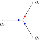
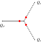
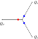
From (16) it can be seen that the three types of three-point interaction vertices are all “derivative interactions”, as shown in Fig.1. This is different from ordinary field theory where fields are locally coupled. Moreover, as we will see, the derivatives bring momentum factors, which will cancel the momentum factors in the denominator come from the two-point correlation functions, and increase the finiteness in IR. Especially, in this work we will show that loop corrections arising from the above three-point vertices are all IR finite.
Refer to caption
Refer to caption
Refer to caption
Figure 1: Diagrammatic representations of three types of adiabatic-entropy three-point cross-interaction vertices. A red dot denotes temporal derivative while a blue dot denotes spatial derivative, or in fourier space, a momentum factor.

There is another issue should be emphasized. In standard slow-roll inflation models, the “effective couplings” of the interaction vertices are greatly suppressed by slow-roll parameters (this is also why primordial non-gaussianies are much small in these models) and thus contributions to the correlation functions from multi-vertices diagrams are suppressed and can be neglected at least in the leading-order. However, this is no longer the case for cs1much-less-thansubscript𝑐𝑠1c_{s}\ll 1 models, where the strength of the interactions are much larger. This can be seen directly from (17), the effective coupling is enhanced by small cssubscript𝑐𝑠c_{s}. For example, in [23], trispectrum from exchanging scalar modes were investigated, it was shown that in cs1much-less-thansubscript𝑐𝑠1c_{s}\ll 1 models, in general the contribution from two-vertices diagrams cannot be neglected in comparison with one-vertices diagrams. The essential idea is that, contributions from diagrams with more numbers of vertices are of the same importance in comparison with contributions from diagrams with less numbers of vertices, even in the leading-order. This is also one of the motivations of this work.

3 One-loop Entropy Mode Corrections

Correlation functions in cosmological context are calculated by using “in-in” formalism [70, 71, 72] (see Appendix A for a brief review). In this work, we focus on the one-loop contributions arising from the three-point vertices, thus we need

Qσ(η,𝒌1)Qσ(η,𝒌2)1loopsubscriptdelimited-⟨⟩subscript𝑄𝜎subscript𝜂subscript𝒌1subscript𝑄𝜎subscript𝜂subscript𝒌21loop\displaystyle\left\langle Q_{\sigma}(\eta_{\ast},\bm{k}_{1})Q_{\sigma}(\eta_{\ast},\bm{k}_{2})\right\rangle_{1-\textrm{loop}} =2Re[+η𝑑η1+η1𝑑η20|Qσ(η,𝒌1)Qσ(η,𝒌2)Hi(η1)Hi(η2)|0]absent2Redelimited-[]subscriptsuperscriptsubscript𝜂superscriptdifferential-dsubscript𝜂1subscriptsuperscriptsubscript𝜂1superscriptdifferential-dsubscript𝜂2quantum-operator-product0subscript𝑄𝜎subscript𝜂subscript𝒌1subscript𝑄𝜎subscript𝜂subscript𝒌2subscript𝐻isubscript𝜂1subscript𝐻isubscript𝜂20\displaystyle=-2\,\textrm{Re}\left[\int^{\eta_{\ast}}_{{-\infty^{+}}}d\eta_{1}\,\int^{\eta_{1}}_{{-\infty^{+}}}d\eta_{2}\,\left\langle 0\left|Q_{\sigma}(\eta_{\ast},\bm{k}_{1})Q_{\sigma}(\eta_{\ast},\bm{k}_{2})\,H_{\textrm{i}}(\eta_{1})\,H_{\textrm{i}}(\eta_{2})\right|0\right\rangle\right] (18)
+η𝑑η1+η𝑑η20|Hi(η1)Qσ(η,𝒌1)Qσ(η,𝒌2)Hi(η2)|0,subscriptsuperscriptsubscript𝜂superscriptdifferential-dsubscript𝜂1subscriptsuperscriptsubscript𝜂superscriptdifferential-dsubscript𝜂2quantum-operator-product0subscript𝐻isubscript𝜂1subscript𝑄𝜎subscript𝜂subscript𝒌1subscript𝑄𝜎subscript𝜂subscript𝒌2subscript𝐻isubscript𝜂20\displaystyle\qquad\qquad+\int^{\eta_{\ast}}_{{-\infty^{-}}}d\eta_{1}\int^{\eta_{\ast}}_{{-\infty^{+}}}d\eta_{2}\,\left\langle 0\left|H_{\textrm{i}}(\eta_{1})\,Q_{\sigma}(\eta_{\ast},\bm{k}_{1})Q_{\sigma}(\eta_{\ast},\bm{k}_{2})\,H_{\textrm{i}}(\eta_{2})\right|0\right\rangle\,,

where we have written explicitly the lower bound for time-integrals333One can refer a recent work [58], for a detailed discussion on the application of “in-in” formalism on cosmological correlation functions, and the issue of the lower bound of time integrals.: ±(1iϵ)superscriptplus-or-minusminus-or-plus1𝑖italic-ϵ-\infty^{\pm}\equiv-\infty(1\mp i\epsilon) (see Appendix A for details). Note that all quantities on the right-hand side in (18) are “interaction-picture” quantities. In this paper we choose Hisubscript𝐻iH_{\textrm{i}} involving three-point cross-interactions of Qσsubscript𝑄𝜎Q_{\sigma} and Qssubscript𝑄𝑠Q_{s} which is given by (15) and (16).

In the following, we neglect the subscript “i” for simplicity. Denote

Qσ(η,𝒌1)Qσ(η,𝒌2)αβ1subscriptdelimited-⟨⟩subscript𝑄𝜎subscript𝜂subscript𝒌1subscript𝑄𝜎subscript𝜂subscript𝒌2𝛼𝛽1\displaystyle{}\left\langle Q_{\sigma}(\eta_{\ast},\bm{k}_{1})Q_{\sigma}(\eta_{\ast},\bm{k}_{2})\right\rangle_{\alpha\beta 1} 2Re[+η𝑑η1+η1𝑑η20|Qσ(η,𝒌1)Qσ(η,𝒌2)Hα(η1)Hβ(η2)|0],absent2Redelimited-[]subscriptsuperscriptsubscript𝜂superscriptdifferential-dsubscript𝜂1subscriptsuperscriptsubscript𝜂1superscriptdifferential-dsubscript𝜂2quantum-operator-product0subscript𝑄𝜎subscript𝜂subscript𝒌1subscript𝑄𝜎subscript𝜂subscript𝒌2subscript𝐻𝛼subscript𝜂1subscript𝐻𝛽subscript𝜂20\displaystyle\equiv-2\,\textrm{Re}\left[\int^{\eta_{\ast}}_{{-\infty^{+}}}d\eta_{1}\,\int^{\eta_{1}}_{{-\infty^{+}}}d\eta_{2}\,\left\langle 0\left|Q_{\sigma}(\eta_{\ast},\bm{k}_{1})Q_{\sigma}(\eta_{\ast},\bm{k}_{2})\,H_{\alpha}(\eta_{1})\,H_{\beta}(\eta_{2})\right|0\right\rangle\right]\,, (19)
Qσ(η,𝒌1)Qσ(η,𝒌2)αβ2subscriptdelimited-⟨⟩subscript𝑄𝜎subscript𝜂subscript𝒌1subscript𝑄𝜎subscript𝜂subscript𝒌2𝛼𝛽2\displaystyle\left\langle Q_{\sigma}(\eta_{\ast},\bm{k}_{1})Q_{\sigma}(\eta_{\ast},\bm{k}_{2})\right\rangle_{\alpha\beta 2} η𝑑η1+η𝑑η20|Hα(η1)Qσ(η,𝒌1)Qσ(η,𝒌2)Hβ(η2)|0,absentsubscriptsuperscriptsubscript𝜂superscriptdifferential-dsubscript𝜂1subscriptsuperscriptsubscript𝜂superscriptdifferential-dsubscript𝜂2quantum-operator-product0subscript𝐻𝛼subscript𝜂1subscript𝑄𝜎subscript𝜂subscript𝒌1subscript𝑄𝜎subscript𝜂subscript𝒌2subscript𝐻𝛽subscript𝜂20\displaystyle\equiv\int^{\eta_{\ast}}_{{-\infty^{-}}}d\eta_{1}\int^{\eta_{\ast}}_{{-\infty^{+}}}d\eta_{2}\,\left\langle 0\left|H_{\alpha}(\eta_{1})\,Q_{\sigma}(\eta_{\ast},\bm{k}_{1})Q_{\sigma}(\eta_{\ast},\bm{k}_{2})\,H_{\beta}(\eta_{2})\right|0\right\rangle\,,

where Hαsubscript𝐻𝛼H_{\alpha}’s are given by (15) and (16). Thus, the final loop-corrections read,

Qσ(η,𝒌1)Qσ(η,𝒌2)1loop=α,β=a,b,ci=12Qσ(η,𝒌1)Qσ(η,𝒌2)αβi.subscriptdelimited-⟨⟩subscript𝑄𝜎subscript𝜂subscript𝒌1subscript𝑄𝜎subscript𝜂subscript𝒌21loopsubscriptformulae-sequence𝛼𝛽𝑎𝑏𝑐superscriptsubscript𝑖12subscriptdelimited-⟨⟩subscript𝑄𝜎subscript𝜂subscript𝒌1subscript𝑄𝜎subscript𝜂subscript𝒌2𝛼𝛽𝑖\left\langle Q_{\sigma}(\eta_{\ast},\bm{k}_{1})Q_{\sigma}(\eta_{\ast},\bm{k}_{2})\right\rangle_{1-\textrm{loop}}=\sum_{\alpha,\beta=a,b,c}\sum_{i=1}^{2}\left\langle Q_{\sigma}(\eta_{\ast},\bm{k}_{1})Q_{\sigma}(\eta_{\ast},\bm{k}_{2})\right\rangle_{\alpha\beta i}\,. (20)

It is useful to note that αβ=βαsubscriptdelimited-⟨⟩𝛼𝛽superscriptsubscriptdelimited-⟨⟩𝛽𝛼\left\langle\cdots\right\rangle_{\alpha\beta}=\left\langle\cdots\right\rangle_{\beta\alpha}^{\ast}.

3.1 Calculating the Loop Corrections

Now we investigate the loop corrections. The calculation is straightforward but rather lengthy. In this section we show the explicit steps. Readers who are interested only in the final loop contributions can go to the next subsection directly.

3.1.1 Diagonal contributions

From (18), the first integral reads,

Qσ(η,𝒌1)Qσ(η,𝒌2)aa12Re[η𝑑η1η1𝑑η20|Qσ(η,𝒌1)Qσ(η,𝒌2)Ha(η1)Ha(η2)|0].subscriptdelimited-⟨⟩subscript𝑄𝜎subscript𝜂subscript𝒌1subscript𝑄𝜎subscript𝜂subscript𝒌2𝑎𝑎12Redelimited-[]subscriptsuperscriptsubscript𝜂differential-dsubscript𝜂1subscriptsuperscriptsubscript𝜂1differential-dsubscript𝜂2quantum-operator-product0subscript𝑄𝜎subscript𝜂subscript𝒌1subscript𝑄𝜎subscript𝜂subscript𝒌2subscript𝐻𝑎subscript𝜂1subscript𝐻𝑎subscript𝜂20{}\left\langle Q_{\sigma}(\eta_{\ast},\bm{k}_{1})Q_{\sigma}(\eta_{\ast},\bm{k}_{2})\right\rangle_{aa1}\equiv-2\,\textrm{Re}\left[\int^{\eta_{\ast}}_{{-\infty}}d\eta_{1}\,\int^{\eta_{1}}_{{-\infty}}d\eta_{2}\,\left\langle 0\left|Q_{\sigma}(\eta_{\ast},\bm{k}_{1})Q_{\sigma}(\eta_{\ast},\bm{k}_{2})\,H_{a}(\eta_{1})\,H_{a}(\eta_{2})\right|0\right\rangle\right]\,. (21)

The integral in the squared-bracket in (21) is

(2π)3δ3(𝒌1+𝒌2) 4g2η𝑑η1η1𝑑η21η1η2ddη1Gk1(η,η1)ddη2Gk1(η,η2)superscript2𝜋3superscript𝛿3subscript𝒌1subscript𝒌24superscript𝑔2subscriptsuperscriptsubscript𝜂differential-dsubscript𝜂1subscriptsuperscriptsubscript𝜂1differential-dsubscript𝜂21subscript𝜂1subscript𝜂2ddsubscript𝜂1subscript𝐺subscript𝑘1subscript𝜂subscript𝜂1ddsubscript𝜂2subscript𝐺subscript𝑘1subscript𝜂subscript𝜂2\displaystyle(2\pi)^{3}\delta^{3}(\bm{k}_{1}+\bm{k}_{2})\;4\,g^{2}\int^{\eta_{\ast}}_{{-\infty}}d\eta_{1}\,\int^{\eta_{1}}_{{-\infty}}d\eta_{2}\,\frac{1}{\eta_{1}\eta_{2}}\,\frac{\textrm{d}}{\textrm{d}\eta_{1}}G_{k_{1}}(\eta_{\ast},\eta_{1})\,\frac{\textrm{d}}{\textrm{d}\eta_{2}}G_{k_{1}}(\eta_{\ast},\eta_{2}) (22)
×d3p(2π)3d2dη1dη2Fp(η1,η2)d2dη1dη2F|𝒑𝒌1|(η1,η2).\displaystyle\qquad\qquad\times\int\frac{d^{3}p}{(2\pi)^{3}}\,\frac{\textrm{d}^{2}}{\textrm{d}\eta_{1}\textrm{d}\eta_{2}}F_{p}(\eta_{1},\eta_{2})\,\frac{\textrm{d}^{2}}{\textrm{d}\eta_{1}\textrm{d}\eta_{2}}F_{|\bm{p}-\bm{k}_{1}|}(\eta_{1},\eta_{2})\,.

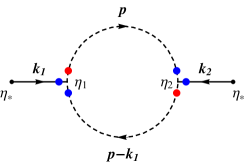
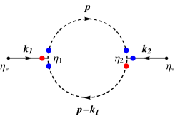
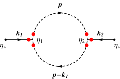
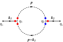
Actually, this expression can be read from the “Feynman-type” diagramatic representation of the contribution, as shown in Fig.2. The main differences from usual field theory is that, here the perturbations are mostly “derivatively-interacted”, rather than in usual field theory the interactions are described by local products of fields. Moreover, in cosmological context, we are interested in the expectation values of some arbitrary time rather than scattering amplitudes. This is why the so-called “in-in” formalism has to be taken. The only thing we should note is the order among three “time” — ηsubscript𝜂\eta_{\ast}, η1subscript𝜂1\eta_{1} and η2subscript𝜂2\eta_{2} between 0|bra0\langle 0| and |0ket0|0\rangle. More precisely, in calculating the first integral of (19), the order is (from left to right) ηsubscript𝜂\eta_{\ast}-η1subscript𝜂1\eta_{1}-η2subscript𝜂2\eta_{2}, while in the second integral in (19), the order is η1subscript𝜂1\eta_{1}-ηsubscript𝜂\eta_{\ast}-η2subscript𝜂2\eta_{2}. Keeping these things in mind, we are able to write the above explicit expressions from Feynman-type diagrams directly.
Refer to caption
Figure 2: Diagrammatic representation of the (aa) loop contributions. A “red dot” denotes derivative with respect to comoving time. It is important to note that the left and right end-points are labeled with ηsubscript𝜂\eta_{\ast}, while the left interaction vertex is labeled with η1subscript𝜂1\eta_{1} and the right vertex is labeled with η2subscript𝜂2\eta_{2}.

Now, from (10) and (12), we have

ddη1Gk1(η,η1)ddη2Gk1(η,η2)ddsubscript𝜂1subscript𝐺subscript𝑘1subscript𝜂subscript𝜂1ddsubscript𝜂2subscript𝐺subscript𝑘1subscript𝜂subscript𝜂2\displaystyle\frac{\textrm{d}}{\textrm{d}\eta_{1}}G_{k_{1}}(\eta_{\ast},\eta_{1})\,\frac{\textrm{d}}{\textrm{d}\eta_{2}}G_{k_{1}}(\eta_{\ast},\eta_{2}) =cs4H44k12η1η2(1+icsk1η)2eicsk1(η1+η22η),absentsuperscriptsubscript𝑐𝑠4superscript𝐻44superscriptsubscript𝑘12subscript𝜂1subscript𝜂2superscript1𝑖subscript𝑐𝑠subscript𝑘1subscript𝜂2superscript𝑒𝑖subscript𝑐𝑠subscript𝑘1subscript𝜂1subscript𝜂22subscript𝜂\displaystyle=\frac{c_{s}^{4}H^{4}}{4k_{1}^{2}}\,\eta_{1}\eta_{2}\left(1+ic_{s}k_{1}\eta_{\ast}\right)^{2}e^{ic_{s}k_{1}\left(\eta_{1}+\eta_{2}-2\eta_{\ast}\right)}\,, (23)
d2dη1dη2Fp(η1,η2)d2dη1dη2F|𝒌2+𝒑|(η1,η2)superscriptd2dsubscript𝜂1dsubscript𝜂2subscript𝐹𝑝subscript𝜂1subscript𝜂2superscriptd2dsubscript𝜂1dsubscript𝜂2subscript𝐹subscript𝒌2𝒑subscript𝜂1subscript𝜂2\displaystyle\frac{\textrm{d}^{2}}{\textrm{d}\eta_{1}\textrm{d}\eta_{2}}F_{p}(\eta_{1},\eta_{2})\,\frac{\textrm{d}^{2}}{\textrm{d}\eta_{1}\textrm{d}\eta_{2}}F_{|\bm{k}_{2}+\bm{p}|}(\eta_{1},\eta_{2}) =cs4H44pη12η22|𝒑+𝒌2|eics(p+|𝒑+𝒌2|)(η1η2).absentsuperscriptsubscript𝑐𝑠4superscript𝐻44𝑝superscriptsubscript𝜂12superscriptsubscript𝜂22𝒑subscript𝒌2superscript𝑒𝑖subscript𝑐𝑠𝑝𝒑subscript𝒌2subscript𝜂1subscript𝜂2\displaystyle=\frac{c_{s}^{4}H^{4}}{4}p\,\eta_{1}^{2}\eta_{2}^{2}\,\left|\bm{p}+\bm{k}_{2}\right|e^{-ic_{s}\left(p+\left|\bm{p}+\bm{k}_{2}\right|\right)(\eta_{1}-\eta_{2})}\,.

Thus, (LABEL:aa1_integral) can be written as

(2π)3δ3(𝒌1+𝒌2)ga2cs8H84k12(1+icsk1η)2e2icsk1ηd3p(2π)3p|𝒑𝒌1|superscript2𝜋3superscript𝛿3subscript𝒌1subscript𝒌2superscriptsubscript𝑔𝑎2superscriptsubscript𝑐𝑠8superscript𝐻84superscriptsubscript𝑘12superscript1𝑖subscript𝑐𝑠subscript𝑘1subscript𝜂2superscript𝑒2𝑖subscript𝑐𝑠subscript𝑘1subscript𝜂superscript𝑑3𝑝superscript2𝜋3𝑝𝒑subscript𝒌1\displaystyle(2\pi)^{3}\delta^{3}(\bm{k}_{1}+\bm{k}_{2})\,g_{a}^{2}\,\frac{c_{s}^{8}H^{8}}{4k_{1}^{2}}\left(1+ic_{s}k_{1}\eta_{\ast}\right)^{2}\,e^{-2ic_{s}k_{1}\eta_{\ast}}\;\int\frac{d^{3}p}{(2\pi)^{3}}\;p\;\left|\bm{p}-\bm{k}_{1}\right| (24)
×ηdη1η12eics(k1p|𝒑𝒌1|)η1η1dη2η22eics(k1+p+|𝒑𝒌1|)η2.\displaystyle\qquad\times\int_{-\infty}^{\eta_{\ast}}d\eta_{1}\;\eta_{1}^{2}\;e^{ic_{s}\left(k_{1}-p-\left|\bm{p}-\bm{k}_{1}\right|\right)\eta_{1}}\int_{-\infty}^{\eta_{1}}d\eta_{2}\;\eta_{2}^{2}\;e^{ic_{s}\left(k_{1}+p+\left|\bm{p}-\bm{k}_{1}\right|\right)\eta_{2}}\,.

The lower bound of both time integrals are -\infty, where the integrants highly oscillate. However, we have to remind ourselves that the lower bound should be chosen carefully in order to choose the true vacuum (see Appendix A for a detailed discussion on this problem and the issue of “choosing vacuum”). Actually, here the lower bound of η1subscript𝜂1\eta_{1} integral and η2subscript𝜂2\eta_{2} integral is the same, +(1iϵ)superscript1𝑖italic-ϵ-\infty^{+}\equiv-\infty(1-i\epsilon). Thus, the time integrals can be evaluated without any ambiguity. For example, the integral w.r.t. η2subscript𝜂2\eta_{2} is evaluated as

(1iϵ)η1𝑑η2η22eics(k1+p+|𝒑𝒌1|)η2=(2i+2csKη1ics2K2η12)eicsKη1cs3K3,superscriptsubscript1𝑖italic-ϵsubscript𝜂1differential-dsubscript𝜂2superscriptsubscript𝜂22superscript𝑒𝑖subscript𝑐𝑠subscript𝑘1𝑝𝒑subscript𝒌1subscript𝜂22𝑖2subscript𝑐𝑠𝐾subscript𝜂1𝑖superscriptsubscript𝑐𝑠2superscript𝐾2superscriptsubscript𝜂12superscript𝑒𝑖subscript𝑐𝑠𝐾subscript𝜂1superscriptsubscript𝑐𝑠3superscript𝐾3\int_{-\infty(1-i\epsilon)}^{\eta_{1}}d\eta_{2}\;\eta_{2}^{2}\;e^{ic_{s}\left(k_{1}+p+\left|\bm{p}-\bm{k}_{1}\right|\right)\eta_{2}}=\frac{\left(2i+2c_{s}K\eta_{1}-ic_{s}^{2}K^{2}\eta_{1}^{2}\right)e^{ic_{s}K\eta_{1}}}{c_{s}^{3}\,K^{3}}\,, (25)

where we write Kk1+p+|𝒑𝒌1|𝐾subscript𝑘1𝑝𝒑subscript𝒌1K\equiv k_{1}+p+\left|\bm{p}-\bm{k}_{1}\right| for simplicity. Thus, after performing the time integrals and taking the real part, we finally get

Qσ(η,𝒌1)Qσ(η,𝒌2)aa1=(2π)3δ3(𝒌1+𝒌2)ga2cs2H816k17d3p(2π)3p|𝒑𝒌1|K3(a1K2+a2KK~+a3K~2),subscriptdelimited-⟨⟩subscript𝑄𝜎subscript𝜂subscript𝒌1subscript𝑄𝜎subscript𝜂subscript𝒌2𝑎𝑎1superscript2𝜋3superscript𝛿3subscript𝒌1subscript𝒌2superscriptsubscript𝑔𝑎2superscriptsubscript𝑐𝑠2superscript𝐻816superscriptsubscript𝑘17superscript𝑑3𝑝superscript2𝜋3𝑝𝒑subscript𝒌1superscript𝐾3subscript𝑎1superscript𝐾2subscript𝑎2𝐾~𝐾subscript𝑎3superscript~𝐾2\displaystyle\left\langle Q_{\sigma}(\eta_{\ast},\bm{k}_{1})Q_{\sigma}(\eta_{\ast},\bm{k}_{2})\right\rangle_{aa1}=-(2\pi)^{3}\,\delta^{3}(\bm{k}_{1}+\bm{k}_{2})\,g_{a}^{2}\,\frac{c_{s}^{2}H^{8}}{16k_{1}^{7}}\int\frac{d^{3}p}{(2\pi)^{3}}\,\frac{p\left|\bm{p}-\bm{k}_{1}\right|}{K^{3}}\,\left(a_{1}K^{2}+a_{2}K\tilde{K}+a_{3}\tilde{K}^{2}\right)\,, (26)

where we have defined K~k1p|𝒑𝒌1|~𝐾subscript𝑘1𝑝𝒑subscript𝒌1\tilde{K}\equiv k_{1}-p-\left|\bm{p}-\bm{k}_{1}\right|, and

a1subscript𝑎1\displaystyle a_{1} 2(2x65x25),absent22superscriptsubscript𝑥65superscriptsubscript𝑥25\displaystyle\equiv 2\,\left(2x_{\ast}^{6}-5x_{\ast}^{2}-5\right)\,, (27)
a2subscript𝑎2\displaystyle a_{2} (2x4+5x2+5),absent2superscriptsubscript𝑥45superscriptsubscript𝑥25\displaystyle\equiv-\left(2x_{\ast}^{4}+5x_{\ast}^{2}+5\right)\,,
a3subscript𝑎3\displaystyle a_{3} (2x4+x2+1),absent2superscriptsubscript𝑥4superscriptsubscript𝑥21\displaystyle\equiv-\left(2x_{\ast}^{4}+x_{\ast}^{2}+1\right)\,,

with xcsk1ηsubscript𝑥subscript𝑐𝑠subscript𝑘1subscript𝜂x_{\ast}\equiv-c_{s}k_{1}\eta_{\ast} for short, note that K+K~=2k1𝐾~𝐾2subscript𝑘1K+\tilde{K}=2k_{1}.

The next step is to evaluate the momentum loop-integral:

I(k)d3p(2π)3p|𝒑𝒌1|K3(a1K2+a2KK~+a3K~2),𝐼𝑘superscript𝑑3𝑝superscript2𝜋3𝑝𝒑subscript𝒌1superscript𝐾3subscript𝑎1superscript𝐾2subscript𝑎2𝐾~𝐾subscript𝑎3superscript~𝐾2{}I(k)\equiv\int\frac{d^{3}p}{(2\pi)^{3}}\,\frac{p\left|\bm{p}-\bm{k}_{1}\right|}{K^{3}}\,\left(a_{1}K^{2}+a_{2}K\tilde{K}+a_{3}\tilde{K}^{2}\right)\,, (28)

remember that Kk1+p+|𝒑𝒌1|𝐾subscript𝑘1𝑝𝒑subscript𝒌1K\equiv k_{1}+p+\left|\bm{p}-\bm{k}_{1}\right| and K~k1p|𝒑𝒌1|~𝐾subscript𝑘1𝑝𝒑subscript𝒌1\tilde{K}\equiv k_{1}-p-\left|\bm{p}-\bm{k}_{1}\right|. Note that the integral (28) is IR finite, thus we do not need to introduce infrared cutoff 1superscript1\ell^{-1} here. It will be shown in this work that loop corrections from the three-point vertices from (16) are all IR finite, due to the “derivatively-coupling” of the perturbations. The integrant in (28) has the structure f(k1,p,|𝒑𝒌1|)𝑓subscript𝑘1𝑝𝒑subscript𝒌1f(k_{1},p,\left|\bm{p}-\bm{k}_{1}\right|), in Appendix B, we describe the method to evaluate such type of integrals. In particular, here the function f(k1,p,|𝒑𝒌1|)𝑓subscript𝑘1𝑝𝒑subscript𝒌1f(k_{1},p,\left|\bm{p}-\bm{k}_{1}\right|) is

f(k1,p,|𝒑𝒌1|)=p|𝒑𝒌1|K3(a1K2+a2KK~+a3K~2).𝑓subscript𝑘1𝑝𝒑subscript𝒌1𝑝𝒑subscript𝒌1superscript𝐾3subscript𝑎1superscript𝐾2subscript𝑎2𝐾~𝐾subscript𝑎3superscript~𝐾2f(k_{1},p,\left|\bm{p}-\bm{k}_{1}\right|)=\frac{p\left|\bm{p}-\bm{k}_{1}\right|}{K^{3}}\,\left(a_{1}K^{2}+a_{2}K\tilde{K}+a_{3}\tilde{K}^{2}\right)\,.

After a straightforward but tedious calculation, we get

Qσ(η,𝒌1)Qσ(η,𝒌2)aa1=(2π)3δ3(𝒌1+𝒌2)Pσ(k1)H2π2ϵcs5(c1lnk+α1),subscriptdelimited-⟨⟩subscript𝑄𝜎subscript𝜂subscript𝒌1subscript𝑄𝜎subscript𝜂subscript𝒌2𝑎𝑎1superscript2𝜋3superscript𝛿3subscript𝒌1subscript𝒌2subscript𝑃𝜎subscript𝑘1superscriptsubscript𝐻2superscript𝜋2italic-ϵsuperscriptsubscript𝑐𝑠5subscript𝑐1𝑘subscript𝛼1{}\left\langle Q_{\sigma}(\eta_{\ast},\bm{k}_{1})Q_{\sigma}(\eta_{\ast},\bm{k}_{2})\right\rangle_{aa1}=(2\pi)^{3}\delta^{3}(\bm{k}_{1}+\bm{k}_{2})P_{\sigma}(k_{1})\frac{H_{\ast}^{2}}{\pi^{2}\epsilon c_{s}^{5}}\left(c_{1}\ln k+\alpha_{1}\right)\,, (29)

where

c1subscript𝑐1\displaystyle c_{1} =44x225x4+x61920,absent44superscriptsubscript𝑥225superscriptsubscript𝑥4superscriptsubscript𝑥61920\displaystyle=\frac{-4-4x_{*}^{2}-25x_{*}^{4}+x_{*}^{6}}{1920}\,, (30)

and α1subscript𝛼1\alpha_{1} denotes the finite part of the momentum integral together with the scheme-dependent UV renormalization constant, which can be found in Appendix C .

Now let us move to the calculation of (aa2)𝑎𝑎2(aa2) contribution. The expression can also be read from fig.2:

Qσ(𝒌1,η)Qσ(𝒌2,η)aa2subscriptdelimited-⟨⟩subscript𝑄𝜎subscript𝒌1subscript𝜂subscript𝑄𝜎subscript𝒌2subscript𝜂𝑎𝑎2\displaystyle\quad\;\left\langle Q_{\sigma}(\bm{k}_{1},\eta_{\ast})Q_{\sigma}(\bm{k}_{2},\eta_{\ast})\right\rangle_{aa2} (31)
=(2π)3δ3(𝒌1+𝒌2) 4g2η𝑑η1η𝑑η21η1η2d3p(2π)3ddη1Gk1(η1,η)ddη2Gk1(η,η2)absentsuperscript2𝜋3superscript𝛿3subscript𝒌1subscript𝒌24superscript𝑔2subscriptsuperscriptsubscript𝜂differential-dsubscript𝜂1subscriptsuperscriptsubscript𝜂differential-dsubscript𝜂21subscript𝜂1subscript𝜂2superscript𝑑3𝑝superscript2𝜋3ddsubscript𝜂1subscript𝐺subscript𝑘1subscript𝜂1subscript𝜂ddsubscript𝜂2subscript𝐺subscript𝑘1subscript𝜂subscript𝜂2\displaystyle=(2\pi)^{3}\delta^{3}(\bm{k}_{1}+\bm{k}_{2})\;4\,g^{2}\int^{\eta_{\ast}}_{{-\infty}}d\eta_{1}\,\int^{\eta_{\ast}}_{{-\infty}}d\eta_{2}\,\frac{1}{\eta_{1}\eta_{2}}\,\int\frac{d^{3}p}{(2\pi)^{3}}\,\frac{\textrm{d}}{\textrm{d}\eta_{1}}G_{k_{1}}(\eta_{1},\eta_{\ast})\,\frac{\textrm{d}}{\textrm{d}\eta_{2}}G_{k_{1}}(\eta_{\ast},\eta_{2})
×d2dη1dη2Fp(η1,η2)d2dη1dη2F|𝒑𝒌1|(η1,η2).absentsuperscriptd2dsubscript𝜂1dsubscript𝜂2subscript𝐹𝑝subscript𝜂1subscript𝜂2superscriptd2dsubscript𝜂1dsubscript𝜂2subscript𝐹𝒑subscript𝒌1subscript𝜂1subscript𝜂2\displaystyle\qquad\qquad\times\frac{\textrm{d}^{2}}{\textrm{d}\eta_{1}\textrm{d}\eta_{2}}F_{p}(\eta_{1},\eta_{2})\,\frac{\textrm{d}^{2}}{\textrm{d}\eta_{1}\textrm{d}\eta_{2}}F_{|\bm{p}-\bm{k}_{1}|}(\eta_{1},\eta_{2})\,.

It is useful to note that, the only difference of integrant from (aa1)-contribution is that, here in fig.2, the order of time is η1ηη2subscript𝜂1subscript𝜂subscript𝜂2\eta_{1}-\eta_{\ast}-\eta_{2}. That is, what we need to do is to simply change the first Green’s function in (aa1)-case as following

ddη1Gk1(η,η1)ddη1Gk1(η1,η),ddsubscript𝜂1subscript𝐺subscript𝑘1subscript𝜂subscript𝜂1ddsubscript𝜂1subscript𝐺subscript𝑘1subscript𝜂1subscript𝜂\frac{\textrm{d}}{\textrm{d}\eta_{1}}G_{k_{1}}(\eta_{\ast},\eta_{1})\qquad\Rightarrow\qquad\frac{\textrm{d}}{\textrm{d}\eta_{1}}G_{k_{1}}(\eta_{1},\eta_{\ast})\,,

to get the above result. Following the same strategy as above, we finally get

Qσ(𝒌1,η)Qσ(𝒌2,η)aa2=(2π)3δ3(𝒌1+𝒌2)Pσ(k1)H2π2ϵcs5(c2lnk1+α2),subscriptdelimited-⟨⟩subscript𝑄𝜎subscript𝒌1subscript𝜂subscript𝑄𝜎subscript𝒌2subscript𝜂𝑎𝑎2superscript2𝜋3superscript𝛿3subscript𝒌1subscript𝒌2subscript𝑃𝜎subscript𝑘1superscript𝐻2superscript𝜋2italic-ϵsuperscriptsubscript𝑐𝑠5subscript𝑐2subscript𝑘1subscript𝛼2{}\left\langle Q_{\sigma}(\bm{k}_{1},\eta_{\ast})Q_{\sigma}(\bm{k}_{2},\eta_{\ast})\right\rangle_{aa2}=(2\pi)^{3}\delta^{3}(\bm{k}_{1}+\bm{k}_{2})\,P_{\sigma}(k_{1})\frac{H^{2}}{\pi^{2}\epsilon c_{s}^{5}}\left(c_{2}\ln k_{1}+\alpha_{2}\right)\,, (32)

with

c2subscript𝑐2\displaystyle c_{2} =1384x4(1+x2),absent1384superscriptsubscript𝑥41superscriptsubscript𝑥2\displaystyle=\frac{1}{384}x_{*}^{4}\left(1+x_{*}^{2}\right)\,, (33)

and α2subscript𝛼2\alpha_{2} can be found in Appendix C.

Collecting (29) and (32) together, we get the contribution from (aa)-term

Qσ(𝒌1,η)Qσ(𝒌2,η)aa=(2π)3δ3(𝒌1+𝒌2)Pσ(k1)H2π2ϵcs5(caalnk1+αaa),subscriptdelimited-⟨⟩subscript𝑄𝜎subscript𝒌1subscript𝜂subscript𝑄𝜎subscript𝒌2subscript𝜂𝑎𝑎superscript2𝜋3superscript𝛿3subscript𝒌1subscript𝒌2subscript𝑃𝜎subscript𝑘1superscript𝐻2superscript𝜋2italic-ϵsuperscriptsubscript𝑐𝑠5subscript𝑐𝑎𝑎subscript𝑘1subscript𝛼𝑎𝑎{}\left\langle Q_{\sigma}(\bm{k}_{1},\eta_{\ast})Q_{\sigma}(\bm{k}_{2},\eta_{\ast})\right\rangle_{aa}=(2\pi)^{3}\delta^{3}(\bm{k}_{1}+\bm{k}_{2})\,P_{\sigma}(k_{1})\frac{H^{2}}{\pi^{2}\epsilon c_{s}^{5}}\left(c_{aa}\ln k_{1}+\alpha_{aa}\right)\,, (34)

with Pσ(k1)subscript𝑃𝜎subscript𝑘1P_{\sigma}(k_{1}) is the (tree-level) power spectrum of adiabatic mode Qσsubscript𝑄𝜎Q_{\sigma}, and

caasubscript𝑐𝑎𝑎\displaystyle c_{aa} =c1+c2=1960(22x210x4+3x6).absentsubscript𝑐1subscript𝑐2196022superscriptsubscript𝑥210superscriptsubscript𝑥43superscriptsubscript𝑥6\displaystyle=c_{1}+c_{2}=\frac{1}{960}\left(-2-2x_{*}^{2}-10x_{*}^{4}+3x_{*}^{6}\right)\,. (35)

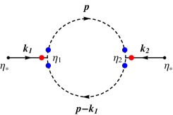
The contributions from (bb)-term can be read from Fig.3.
Refer to caption
Figure 3: Diagrammatic representation of the loop corrections from (bb)-term. As before, a “red dot” denotes derivative with respect to comoving time associated with the vertex, a “blue dot” denotes a momentum factor associated with the line momentum. We may freely label the momentum flows into a vertex a “++” sign and momentum flows out of a vertex a “-” sign. The momentum factors of the same vertex are “scalar-producted”, e.g., the left vertex gives a factor 𝒑(𝒑𝒌1)𝒑𝒑subscript𝒌1-\bm{p}\cdot(\bm{p}-\bm{k}_{1}).
Qσ(𝒌1,η)Qσ(𝒌2,η)bb1subscriptdelimited-⟨⟩subscript𝑄𝜎subscript𝒌1subscript𝜂subscript𝑄𝜎subscript𝒌2subscript𝜂𝑏𝑏1\displaystyle\quad\;\left\langle Q_{\sigma}(\bm{k}_{1},\eta_{\ast})Q_{\sigma}(\bm{k}_{2},\eta_{\ast})\right\rangle_{bb1} (36)
=(2π)3δ3(𝒌1+𝒌2) 8g2cs4×Reη𝑑η1η1𝑑η21η1η2d3p(2π)3[𝒑(𝒑𝒌1)]2absentsuperscript2𝜋3superscript𝛿3subscript𝒌1subscript𝒌28superscript𝑔2superscriptsubscript𝑐𝑠4Resuperscriptsubscriptsubscript𝜂differential-dsubscript𝜂1superscriptsubscriptsubscript𝜂1differential-dsubscript𝜂21subscript𝜂1subscript𝜂2superscript𝑑3𝑝superscript2𝜋3superscriptdelimited-[]𝒑𝒑subscript𝒌12\displaystyle=-(2\pi)^{3}\delta^{3}(\bm{k}_{1}+\bm{k}_{2})\,8\,g^{2}c_{s}^{4}\times\textrm{Re}\int_{-\infty}^{\eta_{\ast}}d\eta_{1}\int_{-\infty}^{\eta_{1}}d\eta_{2}\,\frac{1}{\eta_{1}\eta_{2}}\int\frac{d^{3}p}{(2\pi)^{3}}\left[\bm{p}\cdot(\bm{p}-\bm{k}_{1})\right]^{2}
×ddη1Gk1(η,η1)ddη2Gk1(η,η2)Fp(η1,η2)F|𝒑𝒌1|(η1,η2).absentddsubscript𝜂1subscript𝐺subscript𝑘1subscript𝜂subscript𝜂1ddsubscript𝜂2subscript𝐺subscript𝑘1subscript𝜂subscript𝜂2subscript𝐹𝑝subscript𝜂1subscript𝜂2subscript𝐹𝒑subscript𝒌1subscript𝜂1subscript𝜂2\displaystyle\qquad\qquad\times\frac{\textrm{d}}{\textrm{d}\eta_{1}}G_{k_{1}}(\eta_{\ast},\eta_{1})\,\frac{\textrm{d}}{\textrm{d}\eta_{2}}G_{k_{1}}(\eta_{\ast},\eta_{2})\,F_{p}(\eta_{1},\eta_{2})\,F_{|\bm{p}-\bm{k}_{1}|}(\eta_{1},\eta_{2})\,.

And

Qσ(𝒌1,η)Qσ(𝒌2,η)bb2subscriptdelimited-⟨⟩subscript𝑄𝜎subscript𝒌1subscript𝜂subscript𝑄𝜎subscript𝒌2subscript𝜂𝑏𝑏2\displaystyle\left\langle Q_{\sigma}(\bm{k}_{1},\eta_{\ast})Q_{\sigma}(\bm{k}_{2},\eta_{\ast})\right\rangle_{bb2} =(2π)3δ3(𝒌1+𝒌2) 4g2cs4η𝑑η1η𝑑η21η1η2d3p(2π)3[𝒑(𝒑𝒌1)]2absentsuperscript2𝜋3superscript𝛿3subscript𝒌1subscript𝒌24superscript𝑔2superscriptsubscript𝑐𝑠4superscriptsubscriptsubscript𝜂differential-dsubscript𝜂1superscriptsubscriptsubscript𝜂differential-dsubscript𝜂21subscript𝜂1subscript𝜂2superscript𝑑3𝑝superscript2𝜋3superscriptdelimited-[]𝒑𝒑subscript𝒌12\displaystyle=(2\pi)^{3}\delta^{3}(\bm{k}_{1}+\bm{k}_{2})\,4\,g^{2}c_{s}^{4}\int_{-\infty}^{\eta_{\ast}}d\eta_{1}\int_{-\infty}^{\eta_{\ast}}d\eta_{2}\,\frac{1}{\eta_{1}\eta_{2}}\int\frac{d^{3}p}{(2\pi)^{3}}\left[\bm{p}\cdot(\bm{p}-\bm{k}_{1})\right]^{2} (37)
×ddη1Gk1(η1,η)ddη2Gk1(η,η2)Fp(η1,η2)F|𝒑𝒌1|(η1,η2)absentddsubscript𝜂1subscript𝐺subscript𝑘1subscript𝜂1subscript𝜂ddsubscript𝜂2subscript𝐺subscript𝑘1subscript𝜂subscript𝜂2subscript𝐹𝑝subscript𝜂1subscript𝜂2subscript𝐹𝒑subscript𝒌1subscript𝜂1subscript𝜂2\displaystyle\qquad\qquad\times\frac{\textrm{d}}{\textrm{d}\eta_{1}}G_{k_{1}}(\eta_{1},\eta_{\ast})\,\frac{\textrm{d}}{\textrm{d}\eta_{2}}G_{k_{1}}(\eta_{\ast},\eta_{2})\,F_{p}(\eta_{1},\eta_{2})\,F_{|\bm{p}-\bm{k}_{1}|}(\eta_{1},\eta_{2})

After lengthy but straightforward calculation, we get

Qσ(𝒌1,η)Qσ(𝒌2,η)bb=(2π)3δ3(𝒌1+𝒌2)Pσ(k1)H2π2ϵcs5(cbblnk1+αbb)subscriptdelimited-⟨⟩subscript𝑄𝜎subscript𝒌1subscript𝜂subscript𝑄𝜎subscript𝒌2subscript𝜂𝑏𝑏superscript2𝜋3superscript𝛿3subscript𝒌1subscript𝒌2subscript𝑃𝜎subscript𝑘1superscript𝐻2superscript𝜋2italic-ϵsuperscriptsubscript𝑐𝑠5subscript𝑐𝑏𝑏subscript𝑘1subscript𝛼𝑏𝑏\left\langle Q_{\sigma}(\bm{k}_{1},\eta_{\ast})Q_{\sigma}(\bm{k}_{2},\eta_{\ast})\right\rangle_{bb}=(2\pi)^{3}\delta^{3}(\bm{k}_{1}+\bm{k}_{2})\,P_{\sigma}(k_{1})\frac{H^{2}}{\pi^{2}\epsilon c_{s}^{5}}\left(c_{bb}\ln k_{1}+\alpha_{bb}\right) (38)

with

cbbsubscript𝑐𝑏𝑏\displaystyle c_{bb} =273+27x2+90x48x63840,absent27327superscriptsubscript𝑥290superscriptsubscript𝑥48superscriptsubscript𝑥63840\displaystyle=\frac{-273+27x_{*}^{2}+90x_{*}^{4}-8x_{*}^{6}}{3840}\,, (39)

agian αbbsubscript𝛼𝑏𝑏\alpha_{bb} is the finite part of the momentum integral and can be found in Appendix C.

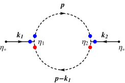
Contributions from (cc)-term can be read from Fig.4.
Refer to caption
Refer to caption
Figure 4: Diagrammatic representation of the loop corrections from (cc)-contribution. As before, a red dot denotes derivative with respect to comoving time associated with the vertex, a blue dot denotes a momentum factor associated with the line momentum. Note that there are two types of diagrams from (cc)-contributions.
Qσ(𝒌1,η)Qσ(𝒌2,η)cc1subscriptdelimited-⟨⟩subscript𝑄𝜎subscript𝒌1subscript𝜂subscript𝑄𝜎subscript𝒌2subscript𝜂𝑐𝑐1\displaystyle\quad\;\left\langle Q_{\sigma}(\bm{k}_{1},\eta_{\ast})Q_{\sigma}(\bm{k}_{2},\eta_{\ast})\right\rangle_{cc1} (40)
=(2π)3δ3(𝒌1+𝒌2) 16g2cs4×Reη𝑑η1η1𝑑η21η1η2d3p(2π)3Gk1(η,η1)Gk1(η,η2)absentsuperscript2𝜋3superscript𝛿3subscript𝒌1subscript𝒌216superscript𝑔2superscriptsubscript𝑐𝑠4Resuperscriptsubscriptsubscript𝜂differential-dsubscript𝜂1superscriptsubscriptsubscript𝜂1differential-dsubscript𝜂21subscript𝜂1subscript𝜂2superscript𝑑3𝑝superscript2𝜋3subscript𝐺subscript𝑘1subscript𝜂subscript𝜂1subscript𝐺subscript𝑘1subscript𝜂subscript𝜂2\displaystyle=-(2\pi)^{3}\delta^{3}(\bm{k}_{1}+\bm{k}_{2})\,16\,g^{2}c_{s}^{4}\times\textrm{Re}\int_{-\infty}^{\eta_{\ast}}d\eta_{1}\int_{-\infty}^{\eta_{1}}d\eta_{2}\,\frac{1}{\eta_{1}\eta_{2}}\int\frac{d^{3}p}{(2\pi)^{3}}\,G_{k_{1}}(\eta_{\ast},\eta_{1})\,G_{k_{1}}(\eta_{\ast},\eta_{2})
×{(𝒑𝒌1)2Fp(η1,η2)d2dη1dη2F|𝒑𝒌1|(η1,η2)\displaystyle\qquad\qquad\times\left\{\left(\bm{p}\cdot\bm{k}_{1}\right)^{2}\,F_{p}(\eta_{1},\eta_{2})\,\frac{\textrm{d}^{2}}{\textrm{d}\eta_{1}\textrm{d}\eta_{2}}F_{|\bm{p}-\bm{k}_{1}|}(\eta_{1},\eta_{2})\right.
(𝒑𝒌1)[𝒌1(𝒑𝒌1)]ddη1Fp(η1,η2)ddη2F|𝒑𝒌1|(η1,η2)}.\displaystyle\qquad\qquad\qquad\left.-\left(\bm{p}\cdot\bm{k}_{1}\right)\,\left[\bm{k}_{1}\cdot(\bm{p}-\bm{k}_{1})\right]\,\frac{\textrm{d}}{\textrm{d}\eta_{1}}F_{p}(\eta_{1},\eta_{2})\,\frac{\textrm{d}}{\textrm{d}\eta_{2}}F_{|\bm{p}-\bm{k}_{1}|}(\eta_{1},\eta_{2})\right\}\,.

And

Qσ(𝒌1,η)Qσ(𝒌2,η)cc2subscriptdelimited-⟨⟩subscript𝑄𝜎subscript𝒌1subscript𝜂subscript𝑄𝜎subscript𝒌2subscript𝜂𝑐𝑐2\displaystyle\quad\;\left\langle Q_{\sigma}(\bm{k}_{1},\eta_{\ast})Q_{\sigma}(\bm{k}_{2},\eta_{\ast})\right\rangle_{cc2} (41)
=(2π)3δ3(𝒌1+𝒌2) 8g2cs4η𝑑η1η𝑑η21η1η2d3p(2π)3Gk1(η1,η)Gk1(η,η2)absentsuperscript2𝜋3superscript𝛿3subscript𝒌1subscript𝒌28superscript𝑔2superscriptsubscript𝑐𝑠4superscriptsubscriptsubscript𝜂differential-dsubscript𝜂1superscriptsubscriptsubscript𝜂differential-dsubscript𝜂21subscript𝜂1subscript𝜂2superscript𝑑3𝑝superscript2𝜋3subscript𝐺subscript𝑘1subscript𝜂1subscript𝜂subscript𝐺subscript𝑘1subscript𝜂subscript𝜂2\displaystyle=(2\pi)^{3}\delta^{3}(\bm{k}_{1}+\bm{k}_{2})\,8\,g^{2}c_{s}^{4}\int_{-\infty}^{\eta_{\ast}}d\eta_{1}\int_{-\infty}^{\eta_{\ast}}d\eta_{2}\,\frac{1}{\eta_{1}\eta_{2}}\int\frac{d^{3}p}{(2\pi)^{3}}\,G_{k_{1}}(\eta_{1},\eta_{\ast})\,G_{k_{1}}(\eta_{\ast},\eta_{2})
×{(𝒑𝒌1)2Fp(η1,η2)d2dη1dη2F|𝒑𝒌1|(η1,η2)\displaystyle\qquad\times\left\{\left(\bm{p}\cdot\bm{k}_{1}\right)^{2}\,F_{p}(\eta_{1},\eta_{2})\,\frac{\textrm{d}^{2}}{\textrm{d}\eta_{1}\textrm{d}\eta_{2}}F_{|\bm{p}-\bm{k}_{1}|}(\eta_{1},\eta_{2})\right.
(𝒑𝒌1)[𝒌1(𝒑𝒌1)]ddη1Fp(η1,η2)ddη2F|𝒑𝒌1|(η1,η2)}.\displaystyle\qquad\qquad\left.-\left(\bm{p}\cdot\bm{k}_{1}\right)\,\left[\bm{k}_{1}\cdot(\bm{p}-\bm{k}_{1})\right]\,\frac{\textrm{d}}{\textrm{d}\eta_{1}}F_{p}(\eta_{1},\eta_{2})\,\frac{\textrm{d}}{\textrm{d}\eta_{2}}F_{|\bm{p}-\bm{k}_{1}|}(\eta_{1},\eta_{2})\right\}\,.

Finally we get

Qσ(𝒌1,η)Qσ(𝒌2,η)cc=(2π)3δ3(𝒌1+𝒌2)Pσ(k1)H2π2ϵcs5(ccclnk1+αcc)subscriptdelimited-⟨⟩subscript𝑄𝜎subscript𝒌1subscript𝜂subscript𝑄𝜎subscript𝒌2subscript𝜂𝑐𝑐superscript2𝜋3superscript𝛿3subscript𝒌1subscript𝒌2subscript𝑃𝜎subscript𝑘1superscript𝐻2superscript𝜋2italic-ϵsuperscriptsubscript𝑐𝑠5subscript𝑐𝑐𝑐subscript𝑘1subscript𝛼𝑐𝑐\left\langle Q_{\sigma}(\bm{k}_{1},\eta_{\ast})Q_{\sigma}(\bm{k}_{2},\eta_{\ast})\right\rangle_{cc}=(2\pi)^{3}\delta^{3}(\bm{k}_{1}+\bm{k}_{2})\,P_{\sigma}(k_{1})\frac{H^{2}}{\pi^{2}\epsilon c_{s}^{5}}\left(c_{cc}\ln k_{1}+\alpha_{cc}\right) (42)

with

cccsubscript𝑐𝑐𝑐\displaystyle c_{cc} =1480[14+x2(7+x2)(2+x2)],absent1480delimited-[]14superscriptsubscript𝑥27superscriptsubscript𝑥22superscriptsubscript𝑥2\displaystyle=\frac{1}{480}\left[-14+x_{*}^{2}\left(-7+x_{*}^{2}\right)\left(2+x_{*}^{2}\right)\right]\,, (43)

and αccsubscript𝛼𝑐𝑐\alpha_{cc} can be found in Appendix C.

3.1.2 Off-diagonal contributions

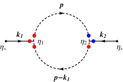
In this work, we consider the one-loop two vertices contributions. Besides the loop contributions from the same vertices, there are contributions involving two different vertices, as shown in Fig.5. As described in the previous section, their explicit expressions can be read from these Feynman-type diagrammatic representations.
Refer to caption
Refer to caption
Refer to caption
Figure 5: Diagrammatic representations of off-diagonal contributions. From left to right are contributions from (ab), (ac) and (bc) combinations respectively. We do not show the (ba), (ca) and (cb) contributions explicitly.

Contributions from (ab)-term are

Qσ(𝒌1,η)Qσ(𝒌2,η)ab1subscriptdelimited-⟨⟩subscript𝑄𝜎subscript𝒌1subscript𝜂subscript𝑄𝜎subscript𝒌2subscript𝜂𝑎𝑏1\displaystyle\quad\;\left\langle Q_{\sigma}(\bm{k}_{1},\eta_{\ast})Q_{\sigma}(\bm{k}_{2},\eta_{\ast})\right\rangle_{ab1} (44)
=(2π)3δ3(𝒌1+𝒌2) 8g2cs2×Reη𝑑η1η1𝑑η21η1η2d3p(2π)3[𝒑(𝒑𝒌1)]absentsuperscript2𝜋3superscript𝛿3subscript𝒌1subscript𝒌28superscript𝑔2superscriptsubscript𝑐𝑠2Resuperscriptsubscriptsubscript𝜂differential-dsubscript𝜂1superscriptsubscriptsubscript𝜂1differential-dsubscript𝜂21subscript𝜂1subscript𝜂2superscript𝑑3𝑝superscript2𝜋3delimited-[]𝒑𝒑subscript𝒌1\displaystyle=-(2\pi)^{3}\delta^{3}(\bm{k}_{1}+\bm{k}_{2})\,8g^{2}c_{s}^{2}\times\textrm{Re}\int_{-\infty}^{\eta_{\ast}}d\eta_{1}\int_{-\infty}^{\eta_{1}}d\eta_{2}\,\frac{1}{\eta_{1}\eta_{2}}\int\frac{d^{3}p}{(2\pi)^{3}}\,\left[\bm{p}\cdot(\bm{p}-\bm{k}_{1})\right]
×ddη1Gk1(η,η1)ddη2Gk1(η,η2)ddη1Fp(η1,η2)ddη1F|𝒑𝒌1|(η1,η2).absentddsubscript𝜂1subscript𝐺subscript𝑘1subscript𝜂subscript𝜂1ddsubscript𝜂2subscript𝐺subscript𝑘1subscript𝜂subscript𝜂2ddsubscript𝜂1subscript𝐹𝑝subscript𝜂1subscript𝜂2ddsubscript𝜂1subscript𝐹𝒑subscript𝒌1subscript𝜂1subscript𝜂2\displaystyle\qquad\qquad\times\frac{\textrm{d}}{\textrm{d}\eta_{1}}G_{k_{1}}(\eta_{\ast},\eta_{1})\,\frac{\textrm{d}}{\textrm{d}\eta_{2}}G_{k_{1}}(\eta_{\ast},\eta_{2})\,\frac{\textrm{d}}{\textrm{d}\eta_{1}}F_{p}(\eta_{1},\eta_{2})\,\frac{\textrm{d}}{\textrm{d}\eta_{1}}F_{|\bm{p}-\bm{k}_{1}|}(\eta_{1},\eta_{2})\,.

And

Qσ(𝒌1,η)Qσ(𝒌2,η)ab2subscriptdelimited-⟨⟩subscript𝑄𝜎subscript𝒌1subscript𝜂subscript𝑄𝜎subscript𝒌2subscript𝜂𝑎𝑏2\displaystyle\quad\;\left\langle Q_{\sigma}(\bm{k}_{1},\eta_{\ast})Q_{\sigma}(\bm{k}_{2},\eta_{\ast})\right\rangle_{ab2} (45)
=(2π)3δ3(𝒌1+𝒌2) 4g2cs2η𝑑η1η𝑑η21η1η2d3p(2π)3[𝒑(𝒑𝒌1)]absentsuperscript2𝜋3superscript𝛿3subscript𝒌1subscript𝒌24superscript𝑔2superscriptsubscript𝑐𝑠2superscriptsubscriptsubscript𝜂differential-dsubscript𝜂1superscriptsubscriptsubscript𝜂differential-dsubscript𝜂21subscript𝜂1subscript𝜂2superscript𝑑3𝑝superscript2𝜋3delimited-[]𝒑𝒑subscript𝒌1\displaystyle=(2\pi)^{3}\delta^{3}(\bm{k}_{1}+\bm{k}_{2})\,4g^{2}c_{s}^{2}\int_{-\infty}^{\eta_{\ast}}d\eta_{1}\int_{-\infty}^{\eta_{\ast}}d\eta_{2}\,\frac{1}{\eta_{1}\eta_{2}}\int\frac{d^{3}p}{(2\pi)^{3}}\,\left[\bm{p}\cdot(\bm{p}-\bm{k}_{1})\right]
×ddη1Gk1(η1,η)ddη2Gk1(η,η2)ddη1Fp(η1,η2)ddη1F|𝒑𝒌1|(η1,η2)absentddsubscript𝜂1subscript𝐺subscript𝑘1subscript𝜂1subscript𝜂ddsubscript𝜂2subscript𝐺subscript𝑘1subscript𝜂subscript𝜂2ddsubscript𝜂1subscript𝐹𝑝subscript𝜂1subscript𝜂2ddsubscript𝜂1subscript𝐹𝒑subscript𝒌1subscript𝜂1subscript𝜂2\displaystyle\qquad\qquad\times\frac{\textrm{d}}{\textrm{d}\eta_{1}}G_{k_{1}}(\eta_{1},\eta_{\ast})\,\frac{\textrm{d}}{\textrm{d}\eta_{2}}G_{k_{1}}(\eta_{\ast},\eta_{2})\,\frac{\textrm{d}}{\textrm{d}\eta_{1}}F_{p}(\eta_{1},\eta_{2})\,\frac{\textrm{d}}{\textrm{d}\eta_{1}}F_{|\bm{p}-\bm{k}_{1}|}(\eta_{1},\eta_{2})

The (ba) contributions can be also read from Fig.5 which we do not write down explicitly. Finally, we denote the contributions from (ab) and (ba) combinations as:

Qσ(𝒌1,η)Qσ(𝒌2,η)ab=(2π)3δ3(𝒌1+𝒌2)Pσ(k1)H2π2ϵcs5(cablnk1+αab)subscriptdelimited-⟨⟩subscript𝑄𝜎subscript𝒌1subscript𝜂subscript𝑄𝜎subscript𝒌2subscript𝜂𝑎𝑏superscript2𝜋3superscript𝛿3subscript𝒌1subscript𝒌2subscript𝑃𝜎subscript𝑘1superscript𝐻2superscript𝜋2italic-ϵsuperscriptsubscript𝑐𝑠5subscript𝑐𝑎𝑏subscript𝑘1subscript𝛼𝑎𝑏\left\langle Q_{\sigma}(\bm{k}_{1},\eta_{\ast})Q_{\sigma}(\bm{k}_{2},\eta_{\ast})\right\rangle_{ab}=(2\pi)^{3}\delta^{3}(\bm{k}_{1}+\bm{k}_{2})\,P_{\sigma}(k_{1})\frac{H^{2}}{\pi^{2}\epsilon c_{s}^{5}}\left(c_{ab}\ln k_{1}+\alpha_{ab}\right) (46)

with

cabsubscript𝑐𝑎𝑏\displaystyle c_{ab} =4x610x411x2+493840.absent4superscriptsubscript𝑥610superscriptsubscript𝑥411superscriptsubscript𝑥2493840\displaystyle=\frac{4x_{*}^{6}-10x_{*}^{4}-11x_{*}^{2}+49}{3840}\,. (47)

Contributions from (ac)-term are:

Qσ(𝒌1,η)Qσ(𝒌2,η)ac1subscriptdelimited-⟨⟩subscript𝑄𝜎subscript𝒌1subscript𝜂subscript𝑄𝜎subscript𝒌2subscript𝜂𝑎𝑐1\displaystyle\quad\;\left\langle Q_{\sigma}(\bm{k}_{1},\eta_{\ast})Q_{\sigma}(\bm{k}_{2},\eta_{\ast})\right\rangle_{ac1} (48)
=(2π)3δ3(𝒌1+𝒌2) 16g2cs2×Reη𝑑η1η1𝑑η21η1η2d3p(2π)3(𝒑𝒌1)absentsuperscript2𝜋3superscript𝛿3subscript𝒌1subscript𝒌216superscript𝑔2superscriptsubscript𝑐𝑠2Resuperscriptsubscriptsubscript𝜂differential-dsubscript𝜂1superscriptsubscriptsubscript𝜂1differential-dsubscript𝜂21subscript𝜂1subscript𝜂2superscript𝑑3𝑝superscript2𝜋3𝒑subscript𝒌1\displaystyle=(2\pi)^{3}\delta^{3}(\bm{k}_{1}+\bm{k}_{2})\,16\,g^{2}c_{s}^{2}\times\textrm{Re}\int_{-\infty}^{\eta_{\ast}}d\eta_{1}\int_{-\infty}^{\eta_{1}}d\eta_{2}\,\frac{1}{\eta_{1}\eta_{2}}\int\frac{d^{3}p}{(2\pi)^{3}}\,\left(\bm{p}\cdot\bm{k}_{1}\right)
×ddη1Gk1(η,η1)Gk1(η,η2)ddη1Fp(η1,η2)d2dη1dη2F|𝒑𝒌1|(η1,η2).absentddsubscript𝜂1subscript𝐺subscript𝑘1subscript𝜂subscript𝜂1subscript𝐺subscript𝑘1subscript𝜂subscript𝜂2ddsubscript𝜂1subscript𝐹𝑝subscript𝜂1subscript𝜂2superscriptd2dsubscript𝜂1dsubscript𝜂2subscript𝐹𝒑subscript𝒌1subscript𝜂1subscript𝜂2\displaystyle\qquad\qquad\times\frac{\textrm{d}}{\textrm{d}\eta_{1}}G_{k_{1}}(\eta_{\ast},\eta_{1})\,G_{k_{1}}(\eta_{\ast},\eta_{2})\,\frac{\textrm{d}}{\textrm{d}\eta_{1}}F_{p}(\eta_{1},\eta_{2})\,\frac{\textrm{d}^{2}}{\textrm{d}\eta_{1}\textrm{d}\eta_{2}}F_{|\bm{p}-\bm{k}_{1}|}(\eta_{1},\eta_{2})\,.

And

Qσ(𝒌1,η)Qσ(𝒌2,η)ac2subscriptdelimited-⟨⟩subscript𝑄𝜎subscript𝒌1subscript𝜂subscript𝑄𝜎subscript𝒌2subscript𝜂𝑎𝑐2\displaystyle\quad\;\left\langle Q_{\sigma}(\bm{k}_{1},\eta_{\ast})Q_{\sigma}(\bm{k}_{2},\eta_{\ast})\right\rangle_{ac2} (49)
=(2π)3δ3(𝒌1+𝒌2) 8g2cs2η𝑑η1η𝑑η21η1η2d3p(2π)3(𝒑𝒌1)absentsuperscript2𝜋3superscript𝛿3subscript𝒌1subscript𝒌28superscript𝑔2superscriptsubscript𝑐𝑠2superscriptsubscriptsubscript𝜂differential-dsubscript𝜂1superscriptsubscriptsubscript𝜂differential-dsubscript𝜂21subscript𝜂1subscript𝜂2superscript𝑑3𝑝superscript2𝜋3𝒑subscript𝒌1\displaystyle=-(2\pi)^{3}\delta^{3}(\bm{k}_{1}+\bm{k}_{2})\,8\,g^{2}c_{s}^{2}\int_{-\infty}^{\eta_{\ast}}d\eta_{1}\int_{-\infty}^{\eta_{\ast}}d\eta_{2}\,\frac{1}{\eta_{1}\eta_{2}}\int\frac{d^{3}p}{(2\pi)^{3}}\,\left(\bm{p}\cdot\bm{k}_{1}\right)
×ddη1Gk1(η1,η)Gk1(η,η2)ddη1Fp(η1,η2)d2dη1dη2F|𝒑𝒌1|(η1,η2).absentddsubscript𝜂1subscript𝐺subscript𝑘1subscript𝜂1subscript𝜂subscript𝐺subscript𝑘1subscript𝜂subscript𝜂2ddsubscript𝜂1subscript𝐹𝑝subscript𝜂1subscript𝜂2superscriptd2dsubscript𝜂1dsubscript𝜂2subscript𝐹𝒑subscript𝒌1subscript𝜂1subscript𝜂2\displaystyle\qquad\qquad\times\frac{\textrm{d}}{\textrm{d}\eta_{1}}G_{k_{1}}(\eta_{1},\eta_{\ast})\,G_{k_{1}}(\eta_{\ast},\eta_{2})\,\frac{\textrm{d}}{\textrm{d}\eta_{1}}F_{p}(\eta_{1},\eta_{2})\,\frac{\textrm{d}^{2}}{\textrm{d}\eta_{1}\textrm{d}\eta_{2}}F_{|\bm{p}-\bm{k}_{1}|}(\eta_{1},\eta_{2})\,.

Similarly, we denote the contributions from (ac) and (ca) as

Qσ(𝒌1,η)Qσ(𝒌2,η)ac=(2π)3δ3(𝒌1+𝒌2)Pσ(k1)H2π2ϵcs5(caclnk1+αac)subscriptdelimited-⟨⟩subscript𝑄𝜎subscript𝒌1subscript𝜂subscript𝑄𝜎subscript𝒌2subscript𝜂𝑎𝑐superscript2𝜋3superscript𝛿3subscript𝒌1subscript𝒌2subscript𝑃𝜎subscript𝑘1superscript𝐻2superscript𝜋2italic-ϵsuperscriptsubscript𝑐𝑠5subscript𝑐𝑎𝑐subscript𝑘1subscript𝛼𝑎𝑐\left\langle Q_{\sigma}(\bm{k}_{1},\eta_{\ast})Q_{\sigma}(\bm{k}_{2},\eta_{\ast})\right\rangle_{ac}=(2\pi)^{3}\delta^{3}(\bm{k}_{1}+\bm{k}_{2})\,P_{\sigma}(k_{1})\frac{H^{2}}{\pi^{2}\epsilon c_{s}^{5}}\left(c_{ac}\ln k_{1}+\alpha_{ac}\right) (50)

with

cacsubscript𝑐𝑎𝑐\displaystyle c_{ac} =28x6+6x423x2233840.absent28superscriptsubscript𝑥66superscriptsubscript𝑥423superscriptsubscript𝑥2233840\displaystyle=\frac{-28x_{*}^{6}+6x_{*}^{4}-23x_{*}^{2}-23}{3840}\,. (51)

Contributions from (bc)-term are:

Qσ(𝒌1,η)Qσ(𝒌2,η)bc1subscriptdelimited-⟨⟩subscript𝑄𝜎subscript𝒌1subscript𝜂subscript𝑄𝜎subscript𝒌2subscript𝜂𝑏𝑐1\displaystyle\quad\;\left\langle Q_{\sigma}(\bm{k}_{1},\eta_{\ast})Q_{\sigma}(\bm{k}_{2},\eta_{\ast})\right\rangle_{bc1} (52)
=(2π)3δ3(𝒌1+𝒌2) 16g2cs4×Reη𝑑η1η1𝑑η21η1η2d3p(2π)3[𝒑(𝒑𝒌1)](𝒑𝒌1)absentsuperscript2𝜋3superscript𝛿3subscript𝒌1subscript𝒌216superscript𝑔2superscriptsubscript𝑐𝑠4Resuperscriptsubscriptsubscript𝜂differential-dsubscript𝜂1superscriptsubscriptsubscript𝜂1differential-dsubscript𝜂21subscript𝜂1subscript𝜂2superscript𝑑3𝑝superscript2𝜋3delimited-[]𝒑𝒑subscript𝒌1𝒑subscript𝒌1\displaystyle=(2\pi)^{3}\delta^{3}(\bm{k}_{1}+\bm{k}_{2})\,16\,g^{2}c_{s}^{4}\times\textrm{Re}\int_{-\infty}^{\eta_{\ast}}d\eta_{1}\int_{-\infty}^{\eta_{1}}d\eta_{2}\,\frac{1}{\eta_{1}\eta_{2}}\int\frac{d^{3}p}{(2\pi)^{3}}\,\left[\bm{p}\cdot(\bm{p}-\bm{k}_{1})\right]\left(\bm{p}\cdot\bm{k}_{1}\right)\,
×ddη1Gk1(η,η1)Gk1(η,η2)Fp(η1,η2)ddη2F|𝒑𝒌1|(η1,η2).absentddsubscript𝜂1subscript𝐺subscript𝑘1subscript𝜂subscript𝜂1subscript𝐺subscript𝑘1subscript𝜂subscript𝜂2subscript𝐹𝑝subscript𝜂1subscript𝜂2ddsubscript𝜂2subscript𝐹𝒑subscript𝒌1subscript𝜂1subscript𝜂2\displaystyle\qquad\qquad\times\frac{\textrm{d}}{\textrm{d}\eta_{1}}G_{k_{1}}(\eta_{\ast},\eta_{1})\,G_{k_{1}}(\eta_{\ast},\eta_{2})\,F_{p}(\eta_{1},\eta_{2})\,\frac{\textrm{d}}{\textrm{d}\eta_{2}}F_{|\bm{p}-\bm{k}_{1}|}(\eta_{1},\eta_{2})\,.

And

Qσ(𝒌1,η)Qσ(𝒌2,η)bc2subscriptdelimited-⟨⟩subscript𝑄𝜎subscript𝒌1subscript𝜂subscript𝑄𝜎subscript𝒌2subscript𝜂𝑏𝑐2\displaystyle\quad\;\left\langle Q_{\sigma}(\bm{k}_{1},\eta_{\ast})Q_{\sigma}(\bm{k}_{2},\eta_{\ast})\right\rangle_{bc2} (53)
=(2π)3δ3(𝒌1+𝒌2) 8g2cs4η𝑑η1η𝑑η21η1η2d3p(2π)3[𝒑(𝒑𝒌1)](𝒑𝒌1)absentsuperscript2𝜋3superscript𝛿3subscript𝒌1subscript𝒌28superscript𝑔2superscriptsubscript𝑐𝑠4superscriptsubscriptsubscript𝜂differential-dsubscript𝜂1superscriptsubscriptsubscript𝜂differential-dsubscript𝜂21subscript𝜂1subscript𝜂2superscript𝑑3𝑝superscript2𝜋3delimited-[]𝒑𝒑subscript𝒌1𝒑subscript𝒌1\displaystyle=-(2\pi)^{3}\delta^{3}(\bm{k}_{1}+\bm{k}_{2})\,8\,g^{2}c_{s}^{4}\int_{-\infty}^{\eta_{\ast}}d\eta_{1}\int_{-\infty}^{\eta_{\ast}}d\eta_{2}\,\frac{1}{\eta_{1}\eta_{2}}\int\frac{d^{3}p}{(2\pi)^{3}}\,\left[\bm{p}\cdot(\bm{p}-\bm{k}_{1})\right]\left(\bm{p}\cdot\bm{k}_{1}\right)\,
×ddη1Gk1(η1,η)Gk1(η,η2)Fp(η1,η2)ddη2F|𝒑𝒌1|(η1,η2).absentddsubscript𝜂1subscript𝐺subscript𝑘1subscript𝜂1subscript𝜂subscript𝐺subscript𝑘1subscript𝜂subscript𝜂2subscript𝐹𝑝subscript𝜂1subscript𝜂2ddsubscript𝜂2subscript𝐹𝒑subscript𝒌1subscript𝜂1subscript𝜂2\displaystyle\qquad\qquad\times\frac{\textrm{d}}{\textrm{d}\eta_{1}}G_{k_{1}}(\eta_{1},\eta_{\ast})\,G_{k_{1}}(\eta_{\ast},\eta_{2})\,F_{p}(\eta_{1},\eta_{2})\,\frac{\textrm{d}}{\textrm{d}\eta_{2}}F_{|\bm{p}-\bm{k}_{1}|}(\eta_{1},\eta_{2})\,.

While the total contributions from (bc) and (cb) terms are,

Qσ(𝒌1,η)Qσ(𝒌2,η)bc=(2π)3δ3(𝒌1+𝒌2)Pσ(k1)H2π2ϵcs5(cbclnk1+αbc)subscriptdelimited-⟨⟩subscript𝑄𝜎subscript𝒌1subscript𝜂subscript𝑄𝜎subscript𝒌2subscript𝜂𝑏𝑐superscript2𝜋3superscript𝛿3subscript𝒌1subscript𝒌2subscript𝑃𝜎subscript𝑘1superscript𝐻2superscript𝜋2italic-ϵsuperscriptsubscript𝑐𝑠5subscript𝑐𝑏𝑐subscript𝑘1subscript𝛼𝑏𝑐{}\left\langle Q_{\sigma}(\bm{k}_{1},\eta_{\ast})Q_{\sigma}(\bm{k}_{2},\eta_{\ast})\right\rangle_{bc}=(2\pi)^{3}\delta^{3}(\bm{k}_{1}+\bm{k}_{2})\,P_{\sigma}(k_{1})\frac{H^{2}}{\pi^{2}\epsilon c_{s}^{5}}\left(c_{bc}\ln k_{1}+\alpha_{bc}\right) (54)

with

cbcsubscript𝑐𝑏𝑐\displaystyle c_{bc} =12x6+66x4+147x2+2273840.absent12superscriptsubscript𝑥666superscriptsubscript𝑥4147superscriptsubscript𝑥22273840\displaystyle=\frac{12x_{*}^{6}+66x_{*}^{4}+147x_{*}^{2}+227}{3840}\,. (55)

3.2 Final Results

Collect (34)-(54) together, the final one-loop contributions from entropy mode to the adiabatic power spectrum is

Qσ(η,𝒌1)Qσ(η,𝒌2)1loop=(2π)3δ3(𝒌1+𝒌2)Pσ(𝒌1)H2π2ϵcs5(clnk1+α),subscriptdelimited-⟨⟩subscript𝑄𝜎subscript𝜂subscript𝒌1subscript𝑄𝜎subscript𝜂subscript𝒌21loopsuperscript2𝜋3superscript𝛿3subscript𝒌1subscript𝒌2subscript𝑃𝜎subscript𝒌1superscriptsubscript𝐻2superscript𝜋2italic-ϵsuperscriptsubscript𝑐𝑠5𝑐subscript𝑘1𝛼\left\langle Q_{\sigma}(\eta_{\ast},\bm{k}_{1})Q_{\sigma}(\eta_{\ast},\bm{k}_{2})\right\rangle_{1-\textrm{loop}}=(2\pi)^{3}\delta^{3}(\bm{k}_{1}+\bm{k}_{2})P_{\sigma}(\bm{k}_{1})\frac{H_{\ast}^{2}}{\pi^{2}\epsilon c_{s}^{5}}\left(c\ln k_{1}+\alpha\right)\,, (56)

with

c𝑐\displaystyle c =1960(18x4+5x235).absent196018superscriptsubscript𝑥45superscriptsubscript𝑥235\displaystyle=\frac{1}{960}\left(18x_{*}^{4}+5x_{*}^{2}-35\right)\,. (57)

Note that the above result should be supplemented with a scheme-dependent UV renormalization constant. This result is consistent with previous analysis [50, 51, 52, 53, 54, 55, 56, 57, 58, 59]. In this work, the loop corrections show no IR divergences. This is mainly due to that in cs1much-less-thansubscript𝑐𝑠1c_{s}\ll 1 limit, the leading-order interaction vertices are dominated by “derivatively-coupled” ones, which enhance the IR safety. Moreover, our result agrees with the bound obtained in [76, 77, 78], where perturbation theory breaks down.

4 Conclusion and Discussion

In this work, we calculate the one-loop corrections to the power spectrum of adiabatic mode from three-point adiabatic/entropy cross-interactions, at the time of horizon exiting. As mentioned before, in cs1much-less-thansubscript𝑐𝑠1c_{s}\ll 1 models, there is enhancement of the effective couplings for interaction vertices, thus contributions (higher-order correlations functions and their loop-corrections) from multi-vertices diagrams are in general cannot be neglected. Precisely, one may expected the two-vertices one-loop contributions and the one-vertex one-loop contributions are of the same order. We find that, as the enhancement of non-gaussianities in models with non-canonical kinetic terms due to the enhancement of small speed of sound cssubscript𝑐𝑠c_{s}, the loop corrections are also enhanced by both the slow-roll parameter ϵitalic-ϵ\epsilon and cssubscript𝑐𝑠c_{s}, more precisely, of order H2ϵcs5similar-toabsentsuperscriptsubscript𝐻2italic-ϵsuperscriptsubscript𝑐𝑠5\sim\frac{H_{\ast}^{2}}{\epsilon c_{s}^{5}}. Thus in general, the loop corrections can be large. Moreover, we find that the loop contributions are IR finite. Although in this work we shown these “large” loop effect through explicit calculations, they can be expected by a simple counting of the order of magnitude of the interaction vertices. The point is that, in relatively large parameter region we need to take into account the higher order loop corrections when we discuss models with small cssubscript𝑐𝑠c_{s}, which may be important in the investigation of large non-Gaussianities.

There are several issues to be addressed. Firstly, the perturbations of inflaton fields and thus the correlation functions themselves are not observable directly. What is responsible for the CMB anisotropies and LSS is the curvature perturbation ζ𝜁\zeta. Thus we should combine the perturbations of inflaton fields to yield the perturbation of curvature perturbation long after horizon exiting, e.g. by using δN𝛿𝑁\delta N formalism [73, 74, 75], as in [55]. However, it is well-known that in multiple field inflation models, the curvature perturbation is not conserved on superhorizon scales, or in other words, there are also cross-correlations among different modes after horizon exiting. Due to these reasons, the complete analysis of loop corrections to the curvature perturbation in multi-field models is a complicate task which needs more subsequent work.

In this work, we focus on the three-point adiabatic/entroy cross-interactions. While from (14), in general, there are adiabatic mode self-interactions. Moreover, in multiple-DBI models, these various interaction-vertices give the same order of contributions, both to non-gaussianties and loop corrections. A complete analysis of loop corrections including contributions from adiabatic loops and also the relations with observables (e.g. the curvature perturbation and the CMB anisotropies) are also needed.


Acknowledgements

We would like to thank Xiangdong Ji, Miao Li, Eugene Lim and Tao Wang for useful discussions and comments. XG was supported by the NSFC grant No.10535060/A050207, a NSFC group grant No.10821504 and Ministry of Science and Technology 973 program under grant No.2007CB815401. F. Xu acknowledges the hospitality from the TQHN group at University of Maryland and the support from China’s Ministry of Education.

Appendix A A Brief Review of “In-in” Formalism

A.1 Preliminaries

The “in-in formalism” (also dubbed as “Schwinger-Keldysh formalism”, or “Closed-time path formalism”) [70, 71, 72] is a perturbative approach for solving the evolution of expectation values over a finite time interval. It is therefore ideally suited not only to backgrounds which do not admit an S-matrix description, such as inflationary backgrounds.

In QFT applied in the calculation of S-matrix in particle physics, the goal is to determine the amplitude for a state in the far past |ψket𝜓|\psi\rangle to become some state |ψketsuperscript𝜓|\psi^{\prime}\rangle in the far future,

ψ|S|ψ=ψ(+)|ψ().quantum-operator-productsuperscript𝜓𝑆𝜓inner-productsuperscript𝜓𝜓\langle\psi^{\prime}|S|\psi\rangle=\langle\psi^{\prime}(+\infty)|\psi(-\infty)\rangle\,.

Here, conditions are imposed on the fields at both very early and very late times. This can be done because that in Minkowski spacetime, the states are assumed to be non-interacting at far past and at far future, and thus are usually taken to be the free vacuum, i.e., the vacuum of the free Hamiltonian H0subscript𝐻0H_{0}. The free vacuum are assumed to be in “one-to-one” correspondence with the true vacuum of the whole interacting theory, as we adiabatically turn on and turn off the interactions between t=𝑡t=-\infty and t=+𝑡t=+\infty.

While the physical situation we are considering here is quite different. Instead of specifying the asymptotic conditions both in the far past and far future, we develop a given state forward in time from a specified initial time, which can be chosen as the beginning of inflation. In cosmological context, the initial state are usually chosen as free vacuum, such as Bunch-Davis vacuum, since at very early times when perturbation modes are deep inside the Hubble horizon, according to the equivalence principle, the interaction-picture fields should have the same form as in Minkowski spacetime.

A.2 “In” vacuum

The Hamiltonian can be split into a free part and an interacting part: H=H0+Hi𝐻subscript𝐻0subscript𝐻iH=H_{0}+H_{\textrm{i}}. The time-evolution operator in the interacting picture is well-known

U(η2,η1)=Texp(iη1η2𝑑tHiI(η)),𝑈subscript𝜂2subscript𝜂1T𝑖superscriptsubscriptsubscript𝜂1subscript𝜂2differential-dsuperscript𝑡subscript𝐻iIsuperscript𝜂{}U(\eta_{2},\eta_{1})=\mathrm{T}\exp\left(-i\int_{\eta_{1}}^{\eta_{2}}dt^{\prime}H_{\textrm{i}\mathrm{I}}(\eta^{\prime})\right)\,, (58)

where subscript “II\mathrm{I}” denotes interaction-picture quantities, T is the time-ordering operator. Our present goal is to relate the interacting vacuum at arbitrary time |ΩI(t)ketsubscriptΩI𝑡|\Omega_{\mathrm{I}}(t)\rangle with free vacuum |0Iketsubscript0I|0_{\mathrm{I}}\rangle (e.g., Bunch-Davis vacuum). The trick is standard. First we may expand |ΩI(η)ketsubscriptΩI𝜂|\Omega_{\mathrm{I}}(\eta)\rangle in terms of eigenstates of free Hamiltonian H0subscript𝐻0H_{0}, |ΩI(η)=n|nInI|ΩI(η)ketsubscriptΩI𝜂subscript𝑛ketsubscript𝑛Iinner-productsubscript𝑛IsubscriptΩI𝜂|\Omega_{\mathrm{I}}(\eta)\rangle=\sum_{n}|n_{\mathrm{I}}\rangle\,\langle n_{\mathrm{I}}|\Omega_{\mathrm{I}}(\eta)\rangle, then we evolve |ΩI(η)ketsubscriptΩI𝜂|\Omega_{\mathrm{I}}(\eta)\rangle by using (58)

|ΩI(η2)=U(η2,η1)|ΩI(η1)=|0I0I|ΩI+n1e+iEn(η2η1)|nInI|ΩI(η1).ketsubscriptΩIsubscript𝜂2𝑈subscript𝜂2subscript𝜂1ketsubscriptΩIsubscript𝜂1ketsubscript0Iinner-productsubscript0IsubscriptΩIsubscript𝑛1superscript𝑒𝑖subscript𝐸𝑛subscript𝜂2subscript𝜂1ketsubscript𝑛Iinner-productsubscript𝑛IsubscriptΩIsubscript𝜂1{}|\Omega_{\mathrm{I}}(\eta_{2})\rangle=U(\eta_{2},\eta_{1})|\Omega_{\mathrm{I}}(\eta_{1})\rangle=|0_{\mathrm{I}}\rangle\,\langle 0_{\mathrm{I}}|\Omega_{\mathrm{I}}\rangle+\sum_{n\geq 1}e^{+iE_{n}(\eta_{2}-\eta_{1})}\,|n_{\mathrm{I}}\rangle\,\langle n_{\mathrm{I}}|\Omega_{\mathrm{I}}(\eta_{1})\rangle\,. (59)

From (59), we can immediately see that, if we choose η2=(1iϵ)subscript𝜂21𝑖italic-ϵ\eta_{2}=-\infty(1-i\epsilon), all excited states in (59) are suppressed. Thus we relate interacting vacuum at η=(1iϵ)𝜂1𝑖italic-ϵ\eta=-\infty(1-i\epsilon) with free vacuum |0ket0|0\rangle as

|ΩI((1iϵ))=|0I0I|ΩIketsubscriptΩI1𝑖italic-ϵketsubscript0Iinner-productsubscript0IsubscriptΩI|\Omega_{\mathrm{I}}(-\infty(1-i\epsilon))\rangle=|0_{\mathrm{I}}\rangle\,\langle 0_{\mathrm{I}}|\Omega_{\mathrm{I}}\rangle (60)

Thus, the interacting vacuum at arbitrary time η𝜂\eta is given by

|VAC,inketVACin\displaystyle|\textrm{VAC},\textrm{in}\rangle |ΩI(η)=U(η,(1iϵ))|ΩI((1iϵ))absentketsubscriptΩI𝜂𝑈𝜂1𝑖italic-ϵketsubscriptΩI1𝑖italic-ϵ\displaystyle\equiv|\Omega_{\mathrm{I}}(\eta)\rangle=U(\eta,-\infty(1-i\epsilon))|\Omega_{\mathrm{I}}(-\infty(1-i\epsilon))\rangle (61)
=Texp(i(1iϵ)η𝑑ηHiI(η))|0I0I|ΩI.absentT𝑖subscriptsuperscript𝜂1𝑖italic-ϵdifferential-dsuperscript𝜂subscript𝐻iIsuperscript𝜂ketsubscript0Iinner-productsubscript0IsubscriptΩI\displaystyle=\mathrm{T}\exp\left(-i\int^{\eta}_{-\infty(1-i\epsilon)}d\eta^{\prime}\,H_{\textrm{i}\mathrm{I}}(\eta^{\prime})\right)|0_{\mathrm{I}}\rangle\,\langle 0_{\mathrm{I}}|\Omega_{\mathrm{I}}\rangle\,.

A.3 Expectation values in “in-in” formalism

The expectation value of operator 𝒪^(η)^𝒪𝜂\hat{\mathcal{O}}(\eta) at arbitrary time η𝜂\eta is evaluated as

𝒪^(η)delimited-⟨⟩^𝒪𝜂\displaystyle{}\langle\hat{\mathcal{O}}(\eta)\rangle VAC,in|𝒪^(η)|VAC,inVAC,in|VAC,inabsentquantum-operator-productVACin^𝒪𝜂VACininner-productVACinVACin\displaystyle\equiv\frac{\langle\textrm{VAC},\textrm{in}|\hat{\mathcal{O}}(\eta)|\textrm{VAC},\textrm{in}\rangle}{\langle\textrm{VAC},\textrm{in}|\textrm{VAC},\textrm{in}\rangle} (62)
=0I|T¯exp(i(1+iϵ)η𝑑ηH1I(η))𝒪^I(η)Texp(i(1iϵ)η𝑑ηHiI(η))|0I,absentquantum-operator-productsubscript0I¯T𝑖subscriptsuperscript𝜂1𝑖italic-ϵdifferential-dsuperscript𝜂subscript𝐻1Isuperscript𝜂subscript^𝒪I𝜂T𝑖subscriptsuperscript𝜂1𝑖italic-ϵdifferential-dsuperscript𝜂subscript𝐻iIsuperscript𝜂subscript0I\displaystyle=\left\langle 0_{\mathrm{I}}\left|\bar{\mathrm{T}}\exp\left(i\int^{\eta}_{-\infty{(1+i\epsilon)}}d\eta^{\prime}H_{1\mathrm{I}}(\eta^{\prime})\right)\,\hat{\mathcal{O}}_{\mathrm{I}}(\eta)\,\mathrm{T}\exp\left(-i\int^{\eta}_{-\infty{(1-i\epsilon)}}d\eta^{\prime}H_{\textrm{i}\mathrm{I}}(\eta^{\prime})\right)\right|0_{\mathrm{I}}\right\rangle\,,

where T¯¯T\bar{\textrm{T}} is the anti-time-ordering operator.

For simplicity, we denote (1iϵ)+1𝑖italic-ϵsuperscript-\infty(1-i\epsilon)\equiv-\infty^{+} and (1+iϵ)1𝑖italic-ϵsuperscript-\infty(1+i\epsilon)\equiv-\infty^{-}, since, e.g., +superscript-\infty^{+} has a positive imaginary part. Now let us focus on the time-order in (62). In standard S-matrix calculations, operators between 0|bra0\langle 0| and |0ket0|0\rangle are automatically time-ordered. While in (62), from right to left, the time starts from infinite past, or +superscript-\infty^{+} precisely, to some arbitrary time η𝜂\eta when the expectation value is evaluated, then back to superscript-\infty^{-} again. This time-contour, which is shown in Fig.6, forms a closed-time path, so “in-in” formalism is sometimes called “closed-time path” (CTP) formalism.

Refer to caption
Figure 6: Closed-time path in “in-in” formalism.

A.4 Perturbation theory

The starting point of perturbation theory is the free theory two-point correlation functions. In canonical quantization procedure, we write a scalar field as

ϕ𝒌(η)=u(k,η)a𝒌+u(k,η)a𝒌,subscriptitalic-ϕ𝒌𝜂𝑢𝑘𝜂subscript𝑎𝒌superscript𝑢𝑘𝜂subscriptsuperscript𝑎𝒌\phi_{\bm{k}}(\eta)=u(k,\eta)a_{\bm{k}}+u^{\ast}(k,\eta)a^{{\dagger}}_{-\bm{k}}\,, (63)

where u(k,η)𝑢𝑘𝜂u(k,\eta) is the mode function for ϕ𝒌(η)subscriptitalic-ϕ𝒌𝜂\phi_{\bm{k}}(\eta) (in practice, uk(η)subscript𝑢𝑘𝜂u_{k}(\eta) and uk(η)subscriptsuperscript𝑢𝑘𝜂u^{\ast}_{k}(\eta) are two linear-independent solutions of equation of motion for ϕ𝒌(η)subscriptitalic-ϕ𝒌𝜂\phi_{\bm{k}}(\eta), which are Wroskian normalized and satisfy some initial or asymptotic conditions ).

The free two-point function takes the form

0|ϕ𝒌1(η1)ϕ𝒌2(η2)|0(2π)3δ3(𝒌1+𝒌2)Gk1(η1,η2),quantum-operator-product0subscriptitalic-ϕsubscript𝒌1subscript𝜂1subscriptitalic-ϕsubscript𝒌2subscript𝜂20superscript2𝜋3superscript𝛿3subscript𝒌1subscript𝒌2subscript𝐺subscript𝑘1subscript𝜂1subscript𝜂2{}\left\langle 0\left|\phi_{\bm{k}_{1}}(\eta_{1})\phi_{\bm{k}_{2}}(\eta_{2})\right|0\right\rangle\equiv(2\pi)^{3}\delta^{3}(\bm{k}_{1}+\bm{k}_{2})G_{k_{1}}(\eta_{1},\eta_{2})\,, (64)

with

Gk1(η1,η2)uk1(η1)uk1(η2).subscript𝐺subscript𝑘1subscript𝜂1subscript𝜂2subscript𝑢subscript𝑘1subscript𝜂1subscriptsuperscript𝑢subscript𝑘1subscript𝜂2{}G_{k_{1}}(\eta_{1},\eta_{2})\equiv u_{k_{1}}(\eta_{1})u^{\ast}_{k_{1}}(\eta_{2})\,. (65)

In this work, we take (64) and (65) as the starting point.

Now Taylor expansion of (62) gives

  • 0th-order

    𝒪^(η)(0)=0I|𝒪^I(η)|0I.superscriptdelimited-⟨⟩^𝒪𝜂0quantum-operator-productsubscript0Isubscript^𝒪I𝜂subscript0I{}\left\langle\hat{\mathcal{O}}(\eta)\right\rangle^{(0)}=\langle 0_{\mathrm{I}}|\hat{\mathcal{O}}_{\mathrm{I}}(\eta)|0_{\mathrm{I}}\rangle\,. (66)
  • 1st-order (one interaction vertex)

    𝒪^(η)(1)=2Re[i+η𝑑η0I|𝒪^I(t)HiI(t)|0I].superscriptdelimited-⟨⟩^𝒪𝜂12Redelimited-[]𝑖subscriptsuperscript𝜂superscriptdifferential-dsuperscript𝜂quantum-operator-productsubscript0Isubscript^𝒪I𝑡subscript𝐻iIsuperscript𝑡subscript0I\left\langle\hat{\mathcal{O}}(\eta)\right\rangle^{(1)}=2\,\textrm{Re}\left[-i\,\int^{\eta}_{{-\infty^{+}}}d\eta^{\prime}\,\left\langle 0_{\mathrm{I}}\left|\hat{\mathcal{O}}_{\mathrm{I}}(t)\,H_{\textrm{i}\mathrm{I}}(t^{\prime})\right|0_{\mathrm{I}}\right\rangle\right]\,. (67)
  • 2nd-order (two interaction vetices)

    𝒪^(η)(2)superscriptdelimited-⟨⟩^𝒪𝜂2\displaystyle\left\langle\hat{\mathcal{O}}(\eta)\right\rangle^{(2)} =2Re[+η𝑑η+η𝑑η′′0I|𝒪^I(η)HiI(η)HiI(η′′)|0I]absent2Redelimited-[]subscriptsuperscript𝜂superscriptdifferential-dsuperscript𝜂subscriptsuperscriptsuperscript𝜂superscriptdifferential-dsuperscript𝜂′′quantum-operator-productsubscript0Isubscript^𝒪I𝜂subscript𝐻iIsuperscript𝜂subscript𝐻iIsuperscript𝜂′′subscript0I\displaystyle=-2\,\textrm{Re}\left[\int^{\eta}_{{-\infty^{+}}}d\eta^{\prime}\,\int^{\eta^{\prime}}_{{-\infty^{+}}}d\eta^{\prime\prime}\,\left\langle 0_{\mathrm{I}}\left|\hat{\mathcal{O}}_{\mathrm{I}}(\eta)\,H_{\textrm{i}\mathrm{I}}(\eta^{\prime})\,H_{\textrm{i}\mathrm{I}}(\eta^{\prime\prime})\right|0_{\mathrm{I}}\right\rangle\right] (68)
    +η𝑑η+η𝑑η′′0I|HiI(η)𝒪^I(η)HiI(η′′)|0I.subscriptsuperscript𝜂superscriptdifferential-dsuperscript𝜂subscriptsuperscript𝜂superscriptdifferential-dsuperscript𝜂′′quantum-operator-productsubscript0Isubscript𝐻iIsuperscript𝜂subscript^𝒪I𝜂subscript𝐻iIsuperscript𝜂′′subscript0I\displaystyle\qquad\qquad+\int^{\eta}_{{-\infty^{-}}}d\eta^{\prime}\int^{\eta}_{{-\infty^{+}}}d\eta^{\prime\prime}\,\left\langle 0_{\mathrm{I}}\left|H_{\textrm{i}\mathrm{I}}(\eta^{\prime})\,\hat{\mathcal{O}}_{\mathrm{I}}(\eta)\,H_{\textrm{i}\mathrm{I}}(\eta^{\prime\prime})\right|0_{\mathrm{I}}\right\rangle\,.

Here in this work, since we are considering one-loop contributions from three-point interaction vertices, (68) is needed.

A.5 Positive/negative-fields notation

There is a formulation of “in-in formalism” in terms of “doubled fields” in the literatures, mostly applied in the path-integral formulation. The reason is that, the closed-time path (CTP) is imagined to circle the time axis in the complex η𝜂\eta-plane (see fig.6). Accordingly, we distinguish operator values from the upper and lower branches by labeling a “++” on the upper increasing-time contour and a “-” on the lower decreasing-time contour. Then it is convenient to introduce a new “time-path-ordering operator” TpsubscriptTp\textrm{T}_{\textrm{p}}, which orders operator along the “CTP-path”, as shown in Fig.6. Obviously, TpsubscriptTp\textrm{T}_{\textrm{p}} acts on ``+"``"``+" fields as time-ordering operator T, and acts “-” fields as anti-time-ordering operator T¯¯T\bar{\textrm{T}}. Thus (62) can be recast into a more convenient and familiar form

𝒪^(η)delimited-⟨⟩^𝒪𝜂\displaystyle{}\langle\hat{\mathcal{O}}(\eta)\rangle 0|Tpexp(iη𝑑ηHi(η))𝒪^I(η)Tpexp(iη𝑑ηHi+(η))|0absentquantum-operator-product0subscriptTp𝑖subscriptsuperscript𝜂differential-dsuperscript𝜂subscriptsuperscript𝐻isuperscript𝜂subscript^𝒪I𝜂subscriptTp𝑖subscriptsuperscript𝜂differential-dsuperscript𝜂subscriptsuperscript𝐻isuperscript𝜂0\displaystyle\equiv\left\langle 0\left|\mathrm{T}_{\textrm{p}}\,\exp\left(i\int^{\eta}_{-\infty}d\eta^{\prime}H^{-}_{\textrm{i}}(\eta^{\prime})\right)\,\hat{\mathcal{O}}_{\mathrm{I}}(\eta)\,\mathrm{T}_{\textrm{p}}\exp\left(-i\int^{\eta}_{-\infty}d\eta^{\prime}H^{+}_{\textrm{i}}(\eta^{\prime})\right)\right|0\right\rangle (69)
=0|Tp𝒪^I(η)exp(iη𝑑η[Hi+(η)Hi(η)])|0.absentquantum-operator-product0subscriptTpsubscript^𝒪I𝜂𝑖subscriptsuperscript𝜂differential-dsuperscript𝜂delimited-[]subscriptsuperscript𝐻isuperscript𝜂subscriptsuperscript𝐻isuperscript𝜂0\displaystyle=\left\langle 0\left|\mathrm{T}_{\textrm{p}}\,\hat{\mathcal{O}}_{\mathrm{I}}(\eta)\,\exp\left(-i\int^{\eta}_{-\infty}d\eta^{\prime}\left[H^{+}_{\textrm{i}}(\eta^{\prime})-H^{-}_{\textrm{i}}(\eta^{\prime})\right]\right)\right|0\right\rangle\,.

Now, since we have two types of fields, the contractions between different pairs yields four kinds of correlation functions,

0|Tpϕ𝒌1±(η1)ϕ𝒌2±(η2)|0(2π)3δ3(𝒌1+𝒌2)Gk±±(η1,η2),quantum-operator-product0subscriptTpsubscriptsuperscriptitalic-ϕplus-or-minussubscript𝒌1subscript𝜂1subscriptsuperscriptitalic-ϕplus-or-minussubscript𝒌2subscript𝜂20superscript2𝜋3superscript𝛿3subscript𝒌1subscript𝒌2subscriptsuperscript𝐺plus-or-minusabsentplus-or-minus𝑘subscript𝜂1subscript𝜂2{}\left\langle 0\left|\textrm{T}_{\textrm{p}}\,\phi^{\pm}_{\bm{k}_{1}}(\eta_{1})\phi^{\pm}_{\bm{k}_{2}}(\eta_{2})\right|0\right\rangle\equiv(2\pi)^{3}\delta^{3}(\bm{k}_{1}+\bm{k}_{2})G^{\pm\pm}_{k}(\eta_{1},\eta_{2})\,, (70)

where

Gk++(η1,η2)subscriptsuperscript𝐺absent𝑘subscript𝜂1subscript𝜂2\displaystyle{}G^{++}_{k}(\eta_{1},\eta_{2}) =Gk>(η1,η2)θ(η1η2)+Gk<(η1,η2)θ(η2η1),absentsubscriptsuperscript𝐺𝑘subscript𝜂1subscript𝜂2𝜃subscript𝜂1subscript𝜂2subscriptsuperscript𝐺𝑘subscript𝜂1subscript𝜂2𝜃subscript𝜂2subscript𝜂1\displaystyle=G^{>}_{k}(\eta_{1},\eta_{2})\theta(\eta_{1}-\eta_{2})+G^{<}_{k}(\eta_{1},\eta_{2})\theta(\eta_{2}-\eta_{1})\,, (71)
Gk(η1,η2)subscriptsuperscript𝐺absent𝑘subscript𝜂1subscript𝜂2\displaystyle G^{--}_{k}(\eta_{1},\eta_{2}) =Gk<(η1,η2)θ(η1η2)+Gk>(η1,η2)θ(η2η1),absentsubscriptsuperscript𝐺𝑘subscript𝜂1subscript𝜂2𝜃subscript𝜂1subscript𝜂2subscriptsuperscript𝐺𝑘subscript𝜂1subscript𝜂2𝜃subscript𝜂2subscript𝜂1\displaystyle=G^{<}_{k}(\eta_{1},\eta_{2})\theta(\eta_{1}-\eta_{2})+G^{>}_{k}(\eta_{1},\eta_{2})\theta(\eta_{2}-\eta_{1})\,,
Gk+(η1,η2)subscriptsuperscript𝐺absent𝑘subscript𝜂1subscript𝜂2\displaystyle G^{+-}_{k}(\eta_{1},\eta_{2}) =Gk<(η1,η2),absentsubscriptsuperscript𝐺𝑘subscript𝜂1subscript𝜂2\displaystyle=G^{<}_{k}(\eta_{1},\eta_{2})\,,
Gk+(η1,η2)subscriptsuperscript𝐺absent𝑘subscript𝜂1subscript𝜂2\displaystyle G^{-+}_{k}(\eta_{1},\eta_{2}) =Gk>(η1,η2),absentsubscriptsuperscript𝐺𝑘subscript𝜂1subscript𝜂2\displaystyle=G^{>}_{k}(\eta_{1},\eta_{2})\,,

and

Gk>(η1,η2)subscriptsuperscript𝐺𝑘subscript𝜂1subscript𝜂2\displaystyle{}G^{>}_{k}(\eta_{1},\eta_{2}) uk(η1)uk(η2),absentsubscript𝑢𝑘subscript𝜂1subscriptsuperscript𝑢𝑘subscript𝜂2\displaystyle\equiv u_{k}(\eta_{1})u^{\ast}_{k}(\eta_{2})\,, (72)
Gk<(η1,η2)subscriptsuperscript𝐺𝑘subscript𝜂1subscript𝜂2\displaystyle G^{<}_{k}(\eta_{1},\eta_{2}) uk(η1)uk(η2)(Gk>(η1,η2))Gk>(η2,η1),absentsubscriptsuperscript𝑢𝑘subscript𝜂1subscript𝑢𝑘subscript𝜂2superscriptsubscriptsuperscript𝐺𝑘subscript𝜂1subscript𝜂2subscriptsuperscript𝐺𝑘subscript𝜂2subscript𝜂1\displaystyle\equiv u^{\ast}_{k}(\eta_{1})u_{k}(\eta_{2})\equiv\left(G^{>}_{k}(\eta_{1},\eta_{2})\right)^{\ast}\equiv G^{>}_{k}(\eta_{2},\eta_{1})\,,

are the vacuum Wightman functions. Now the perturbation calculations are standard, after expanding the TpsubscriptTp\textrm{T}_{\textrm{p}}-ordered operator exponential in (69).

The “doubled-field” notation is a convenient “book-marker” in path-integral formulation of “in-in formalism” in order to put everything into “one” exponential, while this notation itself is not necessary in principle. Especially, in operator formalism, there is no need to take this notation at all (see also [58] for a discussion on this point).

Appendix B Momentum Integral

In this work, the momentum loop-integrals have the structure as

I(k)d3p(2π)3f(k,p,|𝒑𝒌|)𝐼𝑘superscript𝑑3𝑝superscript2𝜋3𝑓𝑘𝑝𝒑𝒌{}I(k)\equiv\int\frac{d^{3}p}{(2\pi)^{3}}\,f(k,p,|\bm{p}-\bm{k}|)\, (73)

where 𝒌𝒌\bm{k} is the momentum of external line, and 𝒑𝒑\bm{p} is the loop momentum. In this appendix, we briefly describe the methodology for evaluating such type of integrals.

In general, one may use spherical coordinates (p,θ,ϕ)𝑝𝜃italic-ϕ(p,\theta,\phi) to calculate (73). However, it is more convenient to introduce a new variable

q|𝒑𝒌|=k2+p22kpcosθ,𝑞𝒑𝒌superscript𝑘2superscript𝑝22𝑘𝑝𝜃q\equiv\left|\bm{p}-\bm{k}\right|=\sqrt{k^{2}+p^{2}-2kp\cos\theta}\,, (74)

and change coordinate (p,θ,ϕ)𝑝𝜃italic-ϕ(p,\theta,\phi) into (p,q,ϕ)𝑝𝑞italic-ϕ(p,q,\phi). Note that this can be done only when k0𝑘0k\neq 0. The integral measure is simply d3p=pqkdpdqdϕsuperscript𝑑3𝑝𝑝𝑞𝑘𝑑𝑝𝑑𝑞𝑑italic-ϕd^{3}p=\frac{pq}{k}dp\,dq\,d\phi. Thus, the original integral (73) becomes

I(k)=1(2π)2k0+𝑑p|pk|p+k𝑑qpqf(k,p,q).𝐼𝑘1superscript2𝜋2𝑘superscriptsubscript0differential-d𝑝superscriptsubscript𝑝𝑘𝑝𝑘differential-d𝑞𝑝𝑞𝑓𝑘𝑝𝑞{}I(k)=\frac{1}{(2\pi)^{2}k}\int_{0}^{+\infty}dp\int_{\left|p-k\right|}^{p+k}dq\;p\,q\,f(k,p,q)\,. (75)

The integral region for p𝑝p and q𝑞q is shown in Fig.7.

Refer to caption
Figure 7: Integral region for variables p𝑝p and q𝑞q.

One may use (75) as the starting point. However, it can be seen directly from Fig.7 that sometimes it is more convenient to use “rotated” variables

x𝑥\displaystyle x q+p,yqp,formulae-sequenceabsent𝑞𝑝𝑦𝑞𝑝\displaystyle\equiv q+p\,,\qquad y\equiv q-p\,, (76)
p𝑝\displaystyle p =12(xy),q=12(x+y),formulae-sequenceabsent12𝑥𝑦𝑞12𝑥𝑦\displaystyle=\frac{1}{2}(x-y)\,,\qquad q=\frac{1}{2}(x+y)\,,

with integral measure dpdq=12dxdy𝑑𝑝𝑑𝑞12𝑑𝑥𝑑𝑦dpdq=\frac{1}{2}dxdy. Finally, the integral can be put into the form

I(k)=18(2π)2kk𝑑xkk𝑑y(x2y2)f(k,12(xy),12(x+y)).𝐼𝑘18superscript2𝜋2𝑘superscriptsubscript𝑘differential-d𝑥superscriptsubscript𝑘𝑘differential-d𝑦superscript𝑥2superscript𝑦2𝑓𝑘12𝑥𝑦12𝑥𝑦{}I(k)=\frac{1}{8(2\pi)^{2}k}\int_{k}^{\infty}dx\,\int_{-k}^{k}dy\;\left(x^{2}-y^{2}\right)\,f\left(k,\,\frac{1}{2}(x-y),\,\frac{1}{2}(x+y)\right)\,. (77)

Appendix C Finite parts

For clarity, we collect the finite constant parts of the loop integrals.

α1subscript𝛼1\displaystyle\alpha_{1} =59256ln2(59+256ln2)x2+(4641600ln2)x4+(30+64ln2)x6122880,absent592562592562superscriptsubscript𝑥246416002superscriptsubscript𝑥430642superscriptsubscript𝑥6122880\displaystyle=\frac{-59-256\ln 2-(59+256\ln 2)x_{*}^{2}+(464-1600\ln 2)x_{*}^{4}+(-30+64\ln 2)x_{*}^{6}}{122880}\,, (78)
α2subscript𝛼2\displaystyle\alpha_{2} =(1+x2)(331+30(21+40ln2)x4)460800.absent1superscriptsubscript𝑥23313021402superscriptsubscript𝑥4460800\displaystyle=\frac{\left(1+x_{*}^{2}\right)\left(331+30(-21+40\ln 2)x_{*}^{4}\right)}{460800}\,.
αaasubscript𝛼𝑎𝑎\displaystyle\alpha_{aa} =4393840ln2+(4393840ln2)x2120(37+160ln2)x4+90(33+64ln2)x61843200,absent4393840243938402superscriptsubscript𝑥2120371602superscriptsubscript𝑥49033642superscriptsubscript𝑥61843200\displaystyle=\frac{439-3840\ln 2+(439-3840\ln 2)x_{*}^{2}-120(-37+160\ln 2)x_{*}^{4}+90(-33+64\ln 2)x_{*}^{6}}{1843200}\,,
αbbsubscript𝛼𝑏𝑏\displaystyle\alpha_{bb} =268743680ln2+(34913+4320ln2)x2+360(47+40ln2)x4+(14101280ln2)x6614400,absent26874368023491343202superscriptsubscript𝑥236047402superscriptsubscript𝑥4141012802superscriptsubscript𝑥6614400\displaystyle=\frac{-2687-43680\ln 2+(34913+4320\ln 2)x_{*}^{2}+360(-47+40\ln 2)x_{*}^{4}+(1410-1280\ln 2)x_{*}^{6}}{614400}\,,
αccsubscript𝛼𝑐𝑐\displaystyle\alpha_{cc} =56476720ln2+x2(56476720ln2+60x2(2340ln2+8ln2x2))230400,absent564767202superscriptsubscript𝑥256476720260superscriptsubscript𝑥22340282superscriptsubscript𝑥2230400\displaystyle=\frac{5647-6720\ln 2+x_{*}^{2}\left(5647-6720\ln 2+60x_{*}^{2}\left(23-40\ln 2+8\ln 2x_{*}^{2}\right)\right)}{230400}\,,
αabsubscript𝛼𝑎𝑏\displaystyle\alpha_{ab} =x2(30x2(x2(11+32ln2)45280ln2)111612640ln2)+4439+11760ln2921600,absentsuperscriptsubscript𝑥230superscriptsubscript𝑥2superscriptsubscript𝑥21132245280211161264024439117602921600\displaystyle=\frac{x_{*}^{2}\left(30x_{*}^{2}\left(x_{*}^{2}(11+32\ln 2)-452-80\ln 2\right)-11161-2640\ln 2\right)+4439+11760\ln 2}{921600}\,,
αacsubscript𝛼𝑎𝑐\displaystyle\alpha_{ac} =120x6(28ln211)+20x4(21+36ln2)+x2(6012760ln2)+6012760ln2460800,absent120superscriptsubscript𝑥62821120superscriptsubscript𝑥421362superscriptsubscript𝑥26012760260127602460800\displaystyle=\frac{-120x_{*}^{6}(28\ln 2-11)+20x_{*}^{4}(21+36\ln 2)+x_{*}^{2}(601-2760\ln 2)+601-2760\ln 2}{460800}\,,
αbcsubscript𝛼𝑏𝑐\displaystyle\alpha_{bc} =120x6(12ln219)+60x4(77+132ln2)+x2(17640ln24849)1249+27240ln2460800.absent120superscriptsubscript𝑥61221960superscriptsubscript𝑥4771322superscriptsubscript𝑥217640248491249272402460800\displaystyle=\frac{120x_{*}^{6}(12\ln 2-19)+60x_{*}^{4}(77+132\ln 2)+x_{*}^{2}(17640\ln 2-4849)-1249+27240\ln 2}{460800}\,.

And

α𝛼\displaystyle\alpha x2(6x2(x2+2218ln2)+347+30ln2)+137210ln25760.absentsuperscriptsubscript𝑥26superscriptsubscript𝑥2superscriptsubscript𝑥22218234730213721025760\displaystyle\equiv\frac{x_{*}^{2}\left(-6x_{*}^{2}\left(x_{*}^{2}+22-18\ln 2\right)+347+30\ln 2\right)+137-210\ln 2}{5760}\,. (79)

References

  • [1] E. Komatsu et al. [WMAP Collaboration], Astrophys. J. Suppl.  180, 330 (2009)
  • [2] D. H. Lyth and A. Riotto, Phys. Rept.  314, 1 (1999) [arXiv:hep-ph/9807278].
  • [3] J. M. Maldacena, JHEP 0305, 013 (2003) [arXiv:astro-ph/0210603].
  • [4] N. Bartolo, E. Komatsu, S. Matarrese and A. Riotto, Phys. Rept.  402, 103 (2004) [arXiv:astro-ph/0406398].
  • [5] D. Seery and J. E. Lidsey, JCAP 0506, 003 (2005) [arXiv:astro-ph/0503692].
  • [6] X. Chen, M. x. Huang, S. Kachru and G. Shiu, JCAP 0701, 002 (2007) [arXiv:hep-th/0605045].
  • [7] X. Chen, M. x. Huang and G. Shiu, Phys. Rev.  D 74, 121301 (2006) [arXiv:hep-th/0610235].
  • [8] F. Arroja and K. Koyama, Phys. Rev.  D 77, 083517 (2008) [arXiv:0802.1167 [hep-th]].
  • [9] D. Seery and J. E. Lidsey, JCAP 0509, 011 (2005) [arXiv:astro-ph/0506056].
  • [10] D. Langlois, S. Renaux-Petel, D. A. Steer and T. Tanaka, Phys. Rev.  D 78, 063523 (2008) [arXiv:0806.0336 [hep-th]].
  • [11] D. Langlois, S. Renaux-Petel, D. A. Steer and T. Tanaka, Phys. Rev. Lett.  101, 061301 (2008) [arXiv:0804.3139 [hep-th]].
  • [12] D. A. Easson, R. Gregory, D. F. Mota, G. Tasinato and I. Zavala, JCAP 0802, 010 (2008) [arXiv:0709.2666 [hep-th]].
  • [13] M. x. Huang, G. Shiu and B. Underwood, Phys. Rev.  D 77, 023511 (2008) [arXiv:0709.3299 [hep-th]].
  • [14] F. Arroja, S. Mizuno and K. Koyama, JCAP 0808, 015 (2008) [arXiv:0806.0619 [astro-ph]].
  • [15] Y. F. Cai and W. Xue, arXiv:0809.4134 [hep-th].
  • [16] Y. F. Cai and H. Y. Xia, arXiv:0904.0062 [hep-th].
  • [17] X. Ji and T. Wang, arXiv:0903.0379 [hep-th].
  • [18] Q. G. Huang, arXiv:0904.2649 [hep-th].
  • [19] Q. G. Huang, arXiv:0903.1542 [hep-th].
  • [20] C. Gordon, D. Wands, B. A. Bassett and R. Maartens, Phys. Rev.  D 63, 023506 (2001) [arXiv:astro-ph/0009131].
  • [21] B. A. Bassett, S. Tsujikawa and D. Wands, Rev. Mod. Phys.  78, 537 (2006) [arXiv:astro-ph/0507632].
  • [22] Xian Gao, JCAP 0806, 029 (2008) [arXiv:0804.1055 [astro-ph]].
  • [23] Xian Gao and Bin Hu, arXiv:0903.1920 [astro-ph.CO].
  • [24] V. F. Mukhanov, L. R. W. Abramo and R. H. Brandenberger, Phys. Rev. Lett.  78, 1624 (1997) [arXiv:gr-qc/9609026].
  • [25] L. R. W. Abramo, R. H. Brandenberger and V. F. Mukhanov, Phys. Rev.  D 56, 3248 (1997) [arXiv:gr-qc/9704037].
  • [26] L. R. W. Abramo and R. P. Woodard, Phys. Rev.  D 60, 044010 (1999) [arXiv:astro-ph/9811430].
  • [27] W. Unruh, arXiv:astro-ph/9802323.
  • [28] V. K. Onemli and R. P. Woodard, Class. Quant. Grav.  19, 4607 (2002) [arXiv:gr-qc/0204065].
  • [29] T. Prokopec, O. Tornkvist and R. P. Woodard, Annals Phys.  303, 251 (2003) [arXiv:gr-qc/0205130].
  • [30] T. Prokopec and R. P. Woodard, Am. J. Phys.  72, 60 (2004) [arXiv:astro-ph/0303358].
  • [31] V. K. Onemli and R. P. Woodard, Phys. Rev.  D 70, 107301 (2004) [arXiv:gr-qc/0406098].
  • [32] T. Brunier, V. K. Onemli and R. P. Woodard, Class. Quant. Grav.  22, 59 (2005) [arXiv:gr-qc/0408080].
  • [33] E. O. Kahya and R. P. Woodard, Phys. Rev.  D 72, 104001 (2005) [arXiv:gr-qc/0508015].
  • [34] E. O. Kahya and R. P. Woodard, Phys. Rev.  D 74, 084012 (2006) [arXiv:gr-qc/0608049].
  • [35] E. O. Kahya, V. K. Onemli and R. P. Woodard, arXiv:0904.4811 [gr-qc].
  • [36] R. H. Brandenberger, arXiv:hep-th/0210165.
  • [37] G. Geshnizjani and R. Brandenberger, JCAP 0504, 006 (2005) [arXiv:hep-th/0310265].
  • [38] R. Brandenberger and A. Mazumdar, JCAP 0408, 015 (2004) [arXiv:hep-th/0402205].
  • [39] R. H. Brandenberger and J. Martin, Phys. Rev.  D 71, 023504 (2005) [arXiv:hep-th/0410223].
  • [40] R. H. Brandenberger and C. S. Lam, arXiv:hep-th/0407048.
  • [41] P. Martineau and R. H. Brandenberger, Phys. Rev.  D 72, 023507 (2005) [arXiv:astro-ph/0505236].
  • [42] I. S. Gerstein, R. Jackiw, S. Weinberg and B. W. Lee, Phys. Rev.  D 3, 2486 (1971).
  • [43] D. Boyanovsky, H. J. de Vega and N. G. Sanchez, Nucl. Phys.  B 747, 25 (2006) [arXiv:astro-ph/0503669].
  • [44] D. Boyanovsky, H. J. de Vega and N. G. Sanchez, Phys. Rev.  D 72, 103006 (2005) [arXiv:astro-ph/0507596].
  • [45] K. Chaicherdsakul, Phys. Rev.  D 75, 063522 (2007) [arXiv:hep-th/0611352].
  • [46] B. Losic and W. G. Unruh, Phys. Rev.  D 72, 123510 (2005) [arXiv:gr-qc/0510078].
  • [47] E. O. Kahya and V. K. Onemli, Phys. Rev.  D 76, 043512 (2007) [arXiv:gr-qc/0612026].
  • [48] A. Bilandzic and T. Prokopec, Phys. Rev.  D 76, 103507 (2007) [arXiv:0704.1905 [astro-ph]].
  • [49] S. P. Kim, Mod. Phys. Lett.  A 22, 1921 (2007) [arXiv:astro-ph/0701399].
  • [50] S. Weinberg, Phys. Rev.  D 72, 043514 (2005) [arXiv:hep-th/0506236].
  • [51] S. Weinberg, Phys. Rev.  D 74, 023508 (2006) [arXiv:hep-th/0605244].
  • [52] M. S. Sloth, Nucl. Phys.  B 748, 149 (2006) [arXiv:astro-ph/0604488].
  • [53] M. S. Sloth, Nucl. Phys.  B 775, 78 (2007) [arXiv:hep-th/0612138].
  • [54] D. Seery, JCAP 0711, 025 (2007) [arXiv:0707.3377 [astro-ph]].
  • [55] D. Seery, JCAP 0802, 006 (2008) [arXiv:0707.3378 [astro-ph]].
  • [56] E. Dimastrogiovanni and N. Bartolo, JCAP 0811, 016 (2008) [arXiv:0807.2790 [astro-ph]].
  • [57] P. Adshead, R. Easther and E. A. Lim, arXiv:0809.4008 [hep-th].
  • [58] P. Adshead, R. Easther and E. A. Lim, arXiv:0904.4207 [hep-th].
  • [59] Y. Urakawa and K. i. Maeda, Phys. Rev.  D 78, 064004 (2008) [arXiv:0801.0126 [hep-th]].
  • [60] H. R. S. Cogollo, Y. Rodriguez and C. A. Valenzuela-Toledo, JCAP 0808, 029 (2008) [arXiv:0806.1546 [astro-ph]].
  • [61] Y. Rodriguez and C. A. Valenzuela-Toledo, arXiv:0811.4092 [astro-ph].
  • [62] C. T. Byrnes, K. Y. Choi and L. M. H. Hall, JCAP 0902, 017 (2009) [arXiv:0812.0807 [astro-ph]].
  • [63] D. H. Lyth, JCAP 0712, 016 (2007) [arXiv:0707.0361 [astro-ph]].
  • [64] N. Bartolo, S. Matarrese, M. Pietroni, A. Riotto and D. Seery, JCAP 0801, 015 (2008) [arXiv:0711.4263 [astro-ph]].
  • [65] K. Enqvist, S. Nurmi, D. Podolsky and G. I. Rigopoulos, JCAP 0804, 025 (2008) [arXiv:0802.0395 [astro-ph]].
  • [66] A. Riotto and M. S. Sloth, JCAP 0804, 030 (2008) [arXiv:0801.1845 [hep-ph]].
  • [67] Y. Urakawa and T. Tanaka, arXiv:0902.3209 [hep-th].
  • [68] Y. Urakawa and T. Tanaka, arXiv:0904.4415 [hep-th].
  • [69] T. M. Janssen, S. P. Miao, T. Prokopec and R. P. Woodard, Class. Quant. Grav.  25, 245013 (2008) [arXiv:0808.2449 [gr-qc]].
  • [70] J. S. Schwinger, J. Math. Phys.  2 (1961) 407.
  • [71] E. Calzetta and B. L. Hu, Phys. Rev.  D 35, 495 (1987).
  • [72] R. D. Jordan, Phys. Rev.  D 33, 444 (1986).
  • [73] A. A. Starobinsky, JETP Lett.  42 (1985) 152 [Pisma Zh. Eksp. Teor. Fiz.  42 (1985) 124].
  • [74] M. Sasaki and E. D. Stewart, Prog. Theor. Phys.  95, 71 (1996) [arXiv:astro-ph/9507001].
  • [75] D. H. Lyth, K. A. Malik and M. Sasaki, JCAP 0505, 004 (2005) [arXiv:astro-ph/0411220].
  • [76] S. Shandera, arXiv:0812.0818 [astro-ph].
  • [77] L. Leblond and S. Shandera, JCAP 0808, 007 (2008) [arXiv:0802.2290 [hep-th]].
  • [78] C. Cheung, P. Creminelli, A. L. Fitzpatrick, J. Kaplan and L. Senatore, JHEP 0803, 014 (2008) [arXiv:0709.0293 [hep-th]].
  • [79] Xian Gao and Fanrong Xu, to apear