A Generalized Sznajd Model

Abstract

In the last decade the Sznajd Model has been successfully employed in modeling some properties and scale features of both proportional and majority elections. We propose a new version of the Sznajd model with a generalized bounded confidence rule - a rule that limits the convincing capability of agents and that is essential to allow coexistence of opinions in the stationary state. With an appropriate choice of parameters it can be reduced to previous models. We solved this new model both in a mean-field approach (for an arbitrary number of opinions) and numerically in a Barabási-Albert network (for three and four opinions), studying the transient and the possible stationary states. We built the phase portrait for the special cases of three and four opinions, defining the attractors and their basins of attraction. Through this analysis, we were able to understand and explain discrepancies between mean-field and simulation results obtained in previous works for the usual Sznajd Model with bounded confidence and three opinions. Both the dynamical system approach and our generalized bounded confidence rule are quite general and we think it can be useful to the understanding of other similar models.

I Introduction

The Sznajd model (SM), proposed in 2000 by Sznajd-Weron and Sznajd, is a model that has been successfully employed in the reproduction of some properties observed in the dynamics of opinion propagation in a closed community Sznajd-Weron and Sznajd (2000). It is a very simple Ising-like model, that always leads to a stationary state of consensus, but with a rich transient behavior. Its originality resides in the way the state of the sites evolves: two agreeing sites work together in changing their neighbors’ state, instead of being influenced by the environment like in the voter model Holley and Liggett (1975); Krapivsky and Redner (2003).

This model has been extensively studied, either with its original set of rules, or in a variety of versions in which one or more rules were changed in order to describe or include specific features (see for instance Stauffer (2003)). It was extended to higher dimensional lattices in 2000 Stauffer et al. (2000); Bernardes et al. (2001) and adapted to deal with more than two opinions in networks of different topologies in 2002 Bernardes et al. (2002). Also, in 2002, Stauffer Stauffer (2002) adapted the bounded confidence restriction, first introduced by Defuant Deffuant et al. (2000) and Krause Hegselmann and Krause (2002) in models with continuous opinions, to the discrete Sznajd Model scenario. His numerical simulation results, for the regular square lattice with three opinions, were in disagreement with what was found in 2004 by Schulze Schulze (2004), that solved the same model in a mean-field approach.

In this work we propose a new model, with a distinct way of introducing the idea of limited persuasion among electors in a discrete model, as the SM. With adequate choices of parameters our model restores the set of rules of previous works, allowing comparisons.

We solved the model’s master equation numerically in a mean-field approach and made simulations of the model in a Barabási-Albert network and in a square lattice, looking at the transient behavior, as well as the stationary state. With the aid of dynamical systems techniques, we were able to draw a general picture of its behavior in phase space, identifying its fixed points and basins of attraction, for three and four dimensions. This analysis allowed us to understand the origin of the discrepancies in the results obtained by Stauffer Stauffer (2002) and Schulze Schulze (2004) for three opinions. We also studied the transient behavior of the model for three opinions. Comparing the mean-field time series with the ones from the model in a BA network, we see that they share many features, which does not happen with the square lattice time series.

This paper is organized as follows: In the next section we briefly review the rules and the behavior of the original SM, the new set of rules introduced by Bernardes and co-authors in 2002, the version of the model with bounded confidence introduced by Stauffer in 2002, and finally, present our own model. In section III we solve the new model in the mean-field approach, in the general case of $M$ opinions; in section IV we present simulation results, the detailed phase-portrait in the special cases of three and four opinions and discuss previous results. Finally, in section V, we summarize our conclusions.

II The Sznajd Model

In the original SM Sznajd-Weron and Sznajd (2000), the sites of a chain with periodic boundary conditions represented voters, that could only have opinions (states) $\sigma=\pm 1$. If a pair of adjacent sites had the same opinion, they would convince their neighbors with probability p=1; however, if they disagreed their divergence would be propagated, with the neighbors adopting an opposite opinion. This model always evolves to one of two absorbing states: a ferromagnetic state (consensus state), with all voters with the same opinion, or an anti-ferromagnetic state, in which every site has an opinion that is different from the opinion of its neighbors (only possible if the chain has an even number of sites or the periodic boundary is dropped). The transient, however, displays a rich behavior, that called the attention of some physicists Bernardes et al. (2001).

This model has been extensively studied, either with its original set of rules, or in a variety of versions in which one or more rules were changed in order to describe or include specific features, as the possibility of more than two opinions, diffusion of agents, restrictions in the convincing capability of agents, or different topologies in the network defining the relationship among voters (for a review, see for instance Stauffer (2003)). In most of the works that followed Sznajd-Weron and Sznajd (2000), the divergence propagation rule was abandoned.

II.1 The Sznajd model in complex networks

In Bernardes et al. (2002), Bernardes et al. studied a new version of the SM, that was adapted in order to describe the evolution of $N>2$ opinions in voters located in an arbitrary network. This new model was employed to simulate proportional elections with $M$ candidates in a Barabási-Albert network. In their version, each site could be in one of $M+1$ states, the extra state standing for undecided voters. Some changes were also introduced in the updating rules, the idea being that, at each time step the same average number of neighboring sites were convinced, as in the SM. This can be accomplished by setting the probability that a site convinces another one to $p=1/q$, where $q$ is the degree (number of neighbors) of the convincing site (in the SM, $\;p=1\;$ always). Also, a different set of rules was devised for the undecided voters, that were not able to propagate their lack of opinion but could be convinced by one of its decided neighbors, even if it did not belong to a pair.

More precisely, the model is defined by the following set of rules: Let $\sigma(i,t)$ be the opinion of a site $i$ at time $t$ ($\sigma(i,t)\in\{0,1,\dots,M\}$, where the positive values represent candidates and $\sigma(i,t)=0$ stands for undecided voters). Initially, all $N$ voters are undecided, except for a set of $M$ initial electors (one for each candidate), chosen at random.

The dynamics consists in visiting each voter in a random (non-sequential) order, applying the following rules:

1. A voter $i$ is chosen at random. If it is not undecided ($\sigma(i,t)\neq 0$), a site $j$ is picked up (at random) from the set $\Gamma_{i}$ of neighbors of $i$ and rule II is applied, else nothing happens.

2. If voter $j$ is undecided ($\sigma(j,t)=0$), then $j$ adopts $i$’s opinion with probability $p_{i}=1/\,q_{i}$, where $q_{i}$ is the degree of site $i$.

3. If both $i$ and $j$ have the same opinion, voter $i$ tries to convince each one of its neighbors with probability $p_{i}=\nicefrac{{1}}{{q_{i}}}$;

4. If $i$ and $j$ have different opinions, nothing happens.

Like the original SM, this model always evolves towards a consensus absorbing state, but during the transient this new model displays a power-law distribution of candidates with $v$ votes. This behavior is in agreement with what has been observed in the statistics of real proportional elections Costa-Filho et al. (1999); Gonzáles et al. (2003); Vannucchi (2006).

II.2 Bounded Confidence

In all versions of the SM in which a site $i$ always convinces another one independently of its opinion, the system evolves to an absorbing state, in which only one opinion survives. That is not always the case in real communities. In an attempt to allow the emergence of different factions, Defuant et al. Deffuant et al. (2000), and Hegselmann and Krause Hegselmann and Krause (2002) introduced the idea of bounded confidence for models with continuous opinions ($\sigma\in[0,1]$). The idea is to assume that electors $i$ and $j$, with opinions $\sigma_{i}$ and $\sigma_{j}$, can interact only if $|\sigma_{i}-\sigma_{j}|\leq\epsilon$, that is, if their opinions are close enough. This model also evolves to absorbing states, but now eventually with the coexistence of two or more opinions that do not interact with each other. This rule can be easily adapted to discrete models, as the SM, if opinions are labeled from 1 to $M$ and $\epsilon$ is set to 1.

In 2002 Stauffer studied the SM with bounded confidence in square lattices Stauffer (2002), while Schulze Schulze (2004) studied its mean field version, arriving at different conclusions: In the lattice, Stauffer showed that the model ‘almost always’ evolved to an absorbing state of consensus, while in the mean-field approach presented by Schulze the consensus was achieved only in 50% of the cases; the system ended up in a state of coexistence of opinions in the other cases.

II.3 Generalized bounded confidence rule

In this work we propose a new model with a generalization of the bounded confidence idea. This new model includes, in a single set of rules, the original SM, the complex SM, the SM with bounded confidence proposed by Stauffer, as well as many other possibilities.

In our generalized model, a site with opinion $\sigma^{\prime}$ has a probability $p_{\sigma^{\prime}\rightarrow\sigma}$ of being convinced by another site with opinion $\sigma$. As in previous models, random non-sequential update is employed, and there are no undecided voters. The rules become:

• Choose a voter $i$ at random and a voter $j\in\Gamma_{i}$. If $\sigma_{i}\neq\sigma_{j}$ we do nothing, else we apply rule II^′.

• Site $j$ tries to convince each one of its neighbors $k$ of opinion $\sigma_{j}=\sigma_{i}$ with probability $\displaystyle\frac{p_{\sigma_{k}\rightarrow\sigma_{j}}}{q_{j}}$, where $q_{j}$ is the coordination of site $j$.

Alternatively, rule (II^′) can also be:

• A neighbor $k$ of $j$ is chosen at random and $j$ convinces $k$ with probability $p_{\sigma_{k}\rightarrow\sigma_{j}}$.

Note that no assumptions about the probabilities $p_{\sigma\rightarrow\sigma^{\prime}}$ are made beforehand. If $p_{\sigma\rightarrow\sigma^{\prime}}$ is always 0 or 1, then, with a convenient choice of values, one can recover both the usual SM and the discrete version with bounded confidence introduced by Stauffer.

III Time evolution in a mean-field approach

We can easily write the master equation for the model presented in the last section:

$$\Delta P(\sigma_{k}=\sigma)=\frac{1}{N}\sum_{\sigma^{\prime}}\sum_{j\in\Gamma_{k}}\sum_{i\in\Gamma_{j}}\frac{1}{q_{i}q_{j}}(p_{\sigma^{\prime}\rightarrow\sigma}P(\sigma_{i}=\sigma_{j}=\sigma,\sigma_{k}=\sigma^{\prime})-$$

$$-p_{\sigma\rightarrow\sigma^{\prime}}P(\sigma_{i}=\sigma_{j}=\sigma^{\prime},\sigma_{k}=\sigma)),$$ (1)

where $\Gamma_{X}$ and $q_{X}$ are, respectively, the set of neighbors and the coordination (degree) of site $X$, and $N$ is the total number of sites.

If

$$\eta_{\sigma}=\frac{1}{N}\sum_{i}P(\sigma_{i}=\sigma),$$

in a mean-field approach, the master equation is reduced to

$$\Delta\eta_{\sigma}=\frac{1}{N}\sum_{\sigma^{\prime}}(\eta_{\sigma}^{2}\eta_{\sigma^{\prime}}p_{\sigma^{\prime}\rightarrow\sigma}-\eta_{\sigma^{\prime}}^{2}\eta_{\sigma}p_{\sigma\rightarrow\sigma^{\prime}}),$$

and in the thermodynamic limit ($N\rightarrow\infty$) we have

$$\dot{\eta}_{\sigma}=\sum_{\sigma^{\prime}}(\eta_{\sigma}^{2}\eta_{\sigma^{\prime}}p_{\sigma^{\prime}\rightarrow\sigma}-\eta_{\sigma^{\prime}}^{2}\eta_{\sigma}p_{\sigma\rightarrow\sigma^{\prime}})\,\,\,\forall\,\,\sigma,$$ (2)

where a time-unit corresponds to a Monte Carlo step ($N$ random trials).

We also define $\vec{\eta}=(\eta_{1},\eta_{2},\ldots,\eta_{M})$, $F_{\sigma}(\vec{\eta})=\dot{\eta}_{\sigma}$ and $\vec{F}=(F_{1},F_{2},\ldots,F_{M})$.

As the sum over $\sigma^{\prime}$ in (2) is antisymmetric with respect to $\sigma$ and $\sigma^{\prime}$, we get

$$\sum_{\sigma}\dot{\eta}_{\sigma}=0\Rightarrow\sum_{\sigma}\eta_{\sigma}=\mathrm{constant}.$$ (3)

From the definition of $\eta$ it follows that this constant must be equal to 1. As a consequence, although the flux has $M$ variables, it is restricted to $M-1$ dimensions. This also implies that zero is an eigenvalue of the Jacobian of $\vec{F}$ for all values of $\vec{\eta}$. Also, if $\;\eta_{\sigma}\geq 0\;\,\forall\,\;\sigma$, the negative term of $\dot{\eta}_{\sigma}$ in (2) is proportional to $\eta_{\sigma}$ (and the term multiplying it does not diverge in the limit $\eta_{\sigma}\rightarrow 0$). So the flux is restricted to the region in which all variables are positive (as it should, since $\eta_{\sigma}$ is the probability that a site chosen at random has opinion $\sigma$ in the mean-field).

The region in phase space where $\eta_{\sigma}\geq 0$ and $\sum_{\sigma}\eta_{\sigma}=1$ is a regular simplex, and each vertex $P_{i}$ represents the consensus absorbing state of opinion $i$. The points inside a simplex are unique convex combinations of its vertices, suggesting a nice way of representing the phase space of the problem. The point $P$ that represents the state $(\eta_{1},\eta_{2},\eta_{3},\ldots,\eta_{M})$ is given by

$$P=\sum_{\sigma}\eta_{\sigma}P_{\sigma}.$$

The fixed points of (2) are given by

$$\sum_{\sigma^{\prime}}\eta_{\sigma^{\prime}}(\eta_{\sigma}p_{\sigma^{\prime}\rightarrow\sigma}-\eta_{\sigma^{\prime}}p_{\sigma\rightarrow\sigma^{\prime}})=0\,\,\mathrm{or}\,\,\eta_{\sigma}=0,$$

and the Jacobian matrix of $\vec{F}$, $(\mathcal{J}_{\vec{F}})_{\sigma,\sigma^{\prime}}$ is

$$\begin{split}(\mathcal{J}_{\vec{F}})_{\sigma,\sigma^{\prime}}=&\frac{\partial F_{\sigma}}{\partial\eta_{\sigma^{\prime}}}=\delta_{\sigma,\sigma^{\prime}}\sum_{\sigma^{\prime\prime}}\eta_{\sigma^{\prime\prime}}(\eta_{\sigma}p_{\sigma^{\prime\prime}\rightarrow\sigma}-\eta_{\sigma^{\prime\prime}}p_{\sigma\rightarrow\sigma^{\prime\prime}})+\\ &+\eta_{\sigma}\left(\delta_{\sigma,\sigma^{\prime}}\sum_{\sigma^{\prime\prime}}\eta_{\sigma^{\prime\prime}}p_{\sigma^{\prime\prime}\rightarrow\sigma}+\eta_{\sigma}p_{\sigma^{\prime}\rightarrow\sigma}-2\eta_{\sigma^{\prime}}p_{\sigma\rightarrow\sigma^{\prime}}\right).\end{split}$$

So, in the fixed point, we have:

$$(\mathcal{J}^{*}_{\vec{F}})_{\sigma,\sigma^{\prime}}=\left\{\begin{array}[]{l}\eta_{\sigma}\delta_{\sigma,\sigma^{\prime}}\sum_{\sigma^{\prime\prime}}\eta_{\sigma^{\prime\prime}}p_{\sigma^{\prime\prime}\rightarrow\sigma}+\eta^{2}_{\sigma}p_{\sigma^{\prime}\rightarrow\sigma}-2\eta_{\sigma}\eta_{\sigma^{\prime}}p_{\sigma\rightarrow\sigma^{\prime}}\,\,\mathrm{if}\,\,\eta_{\sigma}\neq 0\\ \\ -\delta_{\sigma,\sigma^{\prime}}\sum_{\sigma^{\prime\prime}}\eta^{2}_{\sigma^{\prime\prime}}p_{\sigma\rightarrow\sigma^{\prime\prime}}\,\,\mathrm{if}\,\,\eta_{\sigma}=0\end{array}\right.$$

From the expression above it is possible to derive the following conclusions:

• Consider first that a fixed point $P^{*}$ lies in the intersection of manifolds of the type $\eta_{\sigma}=0$, so we have (conveniently reordering the variables)

  $$\mathcal{J}^{*}=\begin{bmatrix}\mathcal{J}^{*}_{R}&\mathcal{M}\\ 0&\mathcal{D}\end{bmatrix}$$ (4)

  where $\mathcal{J}^{*}_{R}$ is the Jacobian restricted to the non-zero variables in the fixed point and $\mathcal{D}$ is the Jacobian restricted to the variables equal to zero in the fixed point, which is a diagonal matrix. So for each opinion $\sigma$ such that $\eta_{\sigma}^{*}=0$ we have an associated eigenvalue $\lambda_{\sigma}\leq 0$,

  $$\lambda_{\sigma}=-\sum_{\sigma^{\prime}}(\eta_{\sigma^{\prime}}^{*})^{2}p_{\sigma\rightarrow\sigma^{\prime}}.$$

  It follows from (4) that if $x$ is an eigenvector of $\mathcal{J}^{*}_{R}$ with eigenvalue $\lambda$, then

  $$\begin{bmatrix}\mathcal{J}^{*}_{R}&\mathcal{M}\\ 0&\mathcal{D}\end{bmatrix}.\begin{bmatrix}x\\ 0\end{bmatrix}=\begin{bmatrix}\mathcal{J}^{*}_{R}.x\\ 0\end{bmatrix}=\lambda\begin{bmatrix}x\\ 0\end{bmatrix}.$$

  So these eigenvectors and eigenvalues are the same as if we had a model with fewer opinions. The eigenvectors are also parallel to all the manifolds $\eta_{\sigma}=0$ where $P^{*}$ is. On the other hand, if $\vec{v}^{k}$ is an eigenvector with eigenvalue $\lambda_{k}$ it follows that $\mathcal{J}^{*}\vec{v}^{k}=\lambda_{k}\vec{v}^{k}$. So for coordinate $\sigma$ we have $\,v^{k}_{\sigma}(\lambda_{k}-\lambda_{\sigma})=0$.

  Hence, if $\vec{v}^{k}$ is not parallel to the manifold defined by $\eta_{\sigma}=0$, then we must have $\lambda_{k}=\lambda_{\sigma}\leq 0$.

• We focus now on the possible values that $\lambda_{\sigma}$ may take. If

  $$\eta_{\sigma^{\prime}}^{*}p_{\sigma\rightarrow\sigma^{\prime}}\neq 0,$$ (5)

  for some $\sigma^{\prime}$, then $\lambda_{\sigma}<0$ and the flux, in the neighborhood of $P^{*}$, is attracted to the manifold $\eta_{\sigma}=0$. Note that the condition expressed in eq. (5) is equivalent to saying that there are still sites able to convince a site with opinion $\sigma$.

  On the other hand, if condition (5) is not satisfied, $\lambda_{\sigma}=0$ and we have, for a point arbitrarily close to the fixed point (but outside $\eta_{\sigma}=0$),

  $$\dot{\eta}_{\sigma}\simeq\sum_{\sigma^{\prime}}\eta_{\sigma}^{2}\eta_{\sigma^{\prime}}^{*}p_{\sigma^{\prime}\rightarrow\sigma},$$

  which is the time evolution in second order. Therefore, if there is a $\sigma^{\prime}$ such that $\eta^{*}_{\sigma^{\prime}}p_{\sigma^{\prime}\rightarrow\sigma}\neq 0$, then the manifold $\eta_{\sigma}=0$ is unstable in the neighborhood of the fixed point. If this new condition is also not satisfied, then $\sigma$ inevitably interacts only with opinions that don’t survive in $P^{*}$, which is the third order term.

  Let $\Omega$ be the set of opinions $\sigma$ such that $\eta_{\sigma}=0$ in $P^{*}$, and let $M$ be the manifold $\eta_{\sigma}=0\,\forall\,\sigma\in\Omega$, so $P^{*}\in M$. It follows that, if any opinion in $\Omega$ interacts in second order, then the trajectories are repelled from $M$ in the neighborhood of $P^{*}$. If all of them interact in first order, then the trajectories are attracted to $M$. If they all interact only in third order the model is degenerate, as opinions in $\Omega$ do not interact with opinions outside of it (because of the particular choice of $p_{\sigma\rightarrow\sigma^{\prime}}$). If all opinions in $\Omega$ either interact in first or in third orders the model degenerates asymptotically.

• Suppose now that all probabilities $p_{\sigma\rightarrow\sigma^{\prime}}$ are non zero, meaning that all sites have some chance of convincing any other one. Consider a surface formed by moving the boundary of the simplex inwardly by a sufficiently small amount (but non zero). With the same reasoning presented above, we conclude that the flux must come from the simplex’s inner region, crossing the surface towards the boundary points.

  It follows then that there is an unstable region where all opinions coexist. For $M=3$ (3 opinions) this region is a node.

• Finally, consider a manifold in which all opinions do not interact with each other, that is,

  $$\eta_{\sigma},\eta_{\sigma^{\prime}}\neq 0\Rightarrow p_{\sigma^{\prime}\rightarrow\sigma}=p_{\sigma\rightarrow\sigma^{\prime}}=0.$$

  Every point in this manifold is a fixed point, and so, this manifold may have a basin of attraction.

These arguments give a qualitative idea of the evolution of the model in the mean-field approach. The less relevant opinions disappear quickly, and the system has a high probability of ending up in a state where different and non-interacting opinions coexist (provided these states exist).

IV The special cases of 3 and 4 opinions

In the following sub-sections we will analyze in detail the phase portraits that represent the dynamics of our model in the cases of three and four opinions, in which they can be drawn. We will also present some results about the time evolution of the average number of votes for each candidate (the transient behavior) and make comparisons between the mean-field (integrated master equation) and the simulated model (in BA networks and square lattices).

IV.1 Scenario with three opinions

It follows from (3) that $\eta_{1}+\eta_{2}+\eta_{3}=1$, so that the flux is restricted to an equilateral triangle. A point in this triangle represents uniquely a set of normalized variables $\eta_{1},\eta_{2},\eta_{3}$; the vertices $P_{1}$, $P_{2}$ and $P_{3}$ represent consensus states with opinions 1, 2 and 3 respectively; and the side $A_{i,j}$, connecting $P_{i}$ to $P_{j}$, represents the set of states in which opinions $i$ and $j$ coexist.

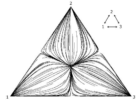
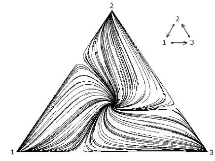
One can show that, if $p_{\sigma\rightarrow\sigma^{\prime}}\neq 0\;\,\forall\,\;\sigma\neq\sigma^{\prime}$, (the usual SM lies in this class) the flux has an unstable node, where all three opinions coexist; three saddle points, in which two opinions coexist; and three stable nodes, representing consensus states (see appendix). Therefore, as far as the convincing power among all different opinions is non-zero, the flux is qualitatively the same and the model will always evolve to an absorbing state of consensus. However, the basins of attraction change, and the same initial condition may belong to different basins if the convincing capabilities change (see figure 1).

(a) Same convincing strength

(b) Asymmetric convincing capability

Figure 1: (a) Phase portrait for the usual Sznajd Model (everybody convinces everyone with equal probabilities), in a mean field approach: there are three stable fixed points (vertices), that correspond to absorbing states of consensus with opinions $1$, $2$ and $3$; three saddle points, in which two opinions coexist, and an unstable node with the coexistence of all three opinions. (b) The scenario described in (a) does not change qualitatively as long as the convincing capability between any two opinions is different from zero. In this picture $p_{1\rightarrow 2}=p_{2\rightarrow 3}=p_{3\rightarrow 1}=0.5$ and $p_{2\rightarrow 1}=p_{3\rightarrow 2}=p_{1\rightarrow 3}=1$. The insets resume the interacting rules; the size of the head of an arrow indicates the strength of the convincing power in that direction.

But what happens when two opinions $\sigma$ and $\sigma^{\prime}$ do not interact? This problem, for $p_{\sigma\rightarrow\sigma^{\prime}}=p_{\sigma^{\prime}\rightarrow\sigma}=0$ if $|\sigma-\sigma^{\prime}|>1$, has already been studied in detail, both numerically Stauffer (2002) (square lattice) and in a mean-field approximation Schulze (2004), with different conclusions. Stauffer showed that, in a square lattice, the stationary state is almost always an absorbing state of consensus in opinion 2. However, Schulze simulated the same model in a complete graph - what corresponds to a mean-field approach - and only in 50% of the simulations the model evolved to the consensus state with opinion 2, found by Stauffer; in the other cases, he observed a steady-state with coexistence of opinions 1 and 3. Our analytical approach and generalized model allow us to to understand why.

In order to understand why the model behaves differently in the mean-field and in the square lattice, we first note that the BA network behaves in the same way as the square lattice, almost always reaching consensus for opinion 2. One would expect the BA network to behave approximately like the mean field, as they both have small world properties, unlike the square lattice. So whatever process causes the lattice to always reach consensus must also be present in the BA network.

To compare the results for the mean-field and the BA network we integrated numerically the equations for the mean-field, to get a phase space portrait of the dynamics. Then, we built an ‘equivalent’ portrait for the stochastic model in a BA network, in the following way: we evolved the model from an initial condition chosen at random, but with specific expected values of $\eta_{1},\eta_{2}$ and $\eta_{3}$, averaging over many simulations. Finally, we plotted the resulting trajectories, together with the mean-field results (see figure 2).

(a)

(b)

Figure 2: Comparison between mean-field trajectories (in gray) and time evolution of the model in a BA network (in black), for the case of three opinions and different combinations of $p_{\sigma\rightarrow\sigma^{\prime}}$. In (a) we have $\epsilon=1$ (usual bounded confidence). The only difference is a slight change in the position of the line that separates the two basins of attraction (see detail of central region in (a)). In (b), $p_{1\rightarrow 2}=p_{1\rightarrow 3}=p_{2\rightarrow 1}=p_{2\rightarrow 3}=p_{3\rightarrow 2}=1$ but $p_{3\rightarrow 1}=0$, i.e. sites with opinion 1 are unable of convincing sites with opinion 3. Note that, in both cases, there is no qualitative change, (actually little quantitative changes) between the phase portraits of the two networks.

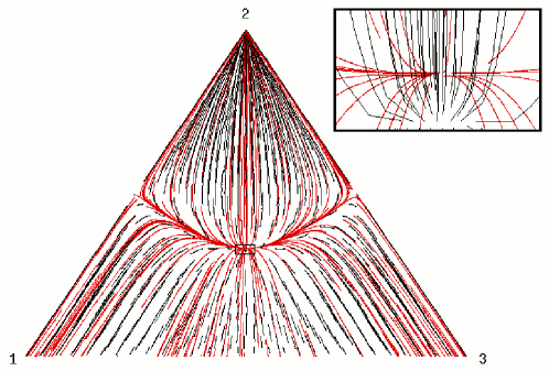
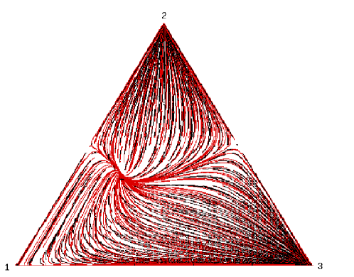
The picture shows that in both cases there are basins of attraction for two kinds of solutions: consensus in opinion 2 or coexistence of opinions 1 and 3. If the initial opinions are drawn at random, with equal probability among opinions 1, 2 and 3, (as done in Stauffer (2002); Schulze (2004)), the initial condition will approximately lay in a circle of radius proportional to $\nicefrac{{1}}{{\sqrt{N}}}$, where $N$ is the number of sites, centered in the point $\eta_{1}=\eta_{2}=\eta_{3}=\nicefrac{{1}}{{3}}$.

In the mean-field scenario, this special point is located on the border of the two basins of attraction. As a consequence, no matter how large is $N$ and, consequently, how small is the neighborhood around the point in which the initial conditions lay, half of its area will be in one basin of attraction and half in the other one.

On the other hand, for the stochastic model this point is, although close to the border, inside the consensus basin of attraction. So the coexistence state can only be achieved for small values of $N$ (small lattices), for which the fluctuations in the initial condition are bigger.

For different choices of $p_{\sigma\rightarrow\sigma^{\prime}}$ the qualitative behavior (fixed points, and basins of attraction) in phase space is only influenced by which of these probabilities are 0 and which are non-zero. When a limit $p_{\sigma\rightarrow\sigma^{\prime}}\rightarrow 0$ is taken, typically there will be some fixed points that collapse to already existing fixed points where fewer opinions coexist. In the example (b) of figure 2 the saddle point between $P_{1}$ and $P_{3}$ (coexistence of 2 opinions) collapses to the node in $P_{1}$ (only 1 opinion) that becomes a saddle.

For all the possibilities where $p_{\sigma\rightarrow\sigma^{\prime}}$ is either 0 or 1, the mean-field approach is able to capture the whole qualitative behavior of the lattice model (see figure 2(b) for instance), even though the trajectories representing the time evolution of the model in a lattice cross each other, what is possible since it is not a flux. This is an assymetric case, for which opinion 1(2) convinces 2(1), opinion 2(3) convinces 3(2), but only opinion 3 is able to change opinion 1 ($p_{3\rightarrow 1}=0$).

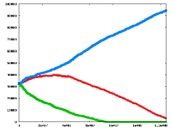
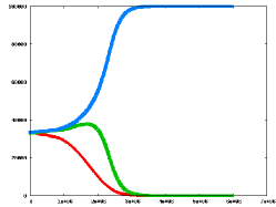
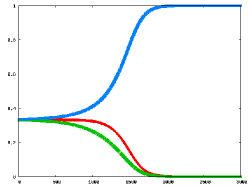
If we study the time evolution of the average number of votes of each candidate, in the three situations studied (square lattice, Barabási-Albert network and mean-field), we see that the mean-filed is a much better approximation for the BA case (see figure 3).

(a)

(b)

(c)

Figure 3: Comparison between the time series of the Sznajd model in different networks and in the absence of bounded confidence. Each color (gray-scale) represents a different opinion. The horizontal axis is time and the vertical one is the number (proportion for the mean field) of voters. Graph (a) is for a square lattice (approximately $10^{5}$ sites), (b) is for a BA network ($10^{6}$ sites and $m=5$) and (c) is for the mean-field. We can see the resemblance of the mean field and the BA network time series.

IV.2 Scenario with four opinions

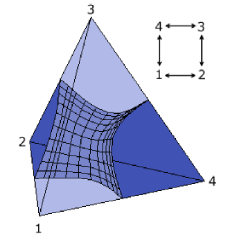
In the case of four opinions, $\eta_{1}+\eta_{2}+\eta_{3}+\eta_{4}=1$, and the flux is restricted to a tetrahedron. With usual bounded confidence rules, $p_{\sigma\rightarrow\sigma^{\prime}}=p_{\sigma^{\prime}\rightarrow\sigma}=0$ if $|\sigma-\sigma^{\prime}|>1$ and $p_{\sigma\rightarrow\sigma^{\prime}}=1$ otherwise. If we add an interaction between opinions 1 and 4 ($p_{1\rightarrow 4}=p_{4\rightarrow 1}=1$), each one of the tetrahedron’s faces reproduces the 3 opinion scenario described in the previous section. By continuity arguments, we can guess that in this case, there are two distinct basins of attraction, shown in figure 4. The internal surface isolates completely region I, that includes the edge $2\Leftrightarrow 4$ from region II, that includes edge $1\Leftrightarrow 3$. As all points of both these edges are fixed points, there are two possible absorbing states with coexistence of opinions (opinions 2 and 4 or opinions 1 and 3), regions I and II are therefore the basins of attraction of these states. The fixed point with coexistence of four opinions (that lies in the surface between I and II) is unstable, the ones with three opinions are saddles (the edges $1\Leftrightarrow 4,2\Leftrightarrow 3,1\Leftrightarrow 2$ and $4\Leftrightarrow 3$ are unstable manifolds) and although the consensus states are in the stable edges ($1\Leftrightarrow 3$ and $2\Leftrightarrow 4$) they are unattainable.

Figure 4: (Color online) Boundary between the 2 basins of attraction for the four opinion model with $\epsilon=1$; different basins are in different gray (blue) tones.

V Conclusions

In summary, we propose a new version of the Sznajd Model, generalizing the bounded confidence rule. We solve the model in a mean-field approach, for a quite general case, discussing some aspects of the dynamics. We showed that the qualitative behavior of trajectories in the mean-field approach can be reduced to the study of the cases $p_{\sigma\rightarrow\sigma^{\prime}}=0$ and $p_{\sigma\rightarrow\sigma^{\prime}}=1$ for each one of the possible pairs of opinions $\sigma$ and $\sigma^{\prime}$. Also, as long as every opinion interacts with all the others, the only possible absorbing state is consensus.

For the special cases of three and four opinions, that had already been studied in the literature, we were able to find a nice way of representing the whole phase space and drew the detailed phase portrait, both in a mean-field approach and for a Barabási-Albert network simulation (in which case we developed a method to draw the stochastic trajectories). In both cases the results are qualitatively the same (in fact, they are remarkably alike), with two distinct basins of attractions: one for an absorbing state of consensus in opinion 2, and another for an absorbing state with coexistence of opinions 1 and 3. The only difference was in the position of the line that separates the two basins of attraction. This picture enabled us to understand why in Schulze (2004) (mean-field), the model ended up in an absorbing state of consensus only in 50% of the cases, while in the numerical simulations on a BA network Stauffer (2002) it almost always ended up in this state.

Also, regarding the whole time evolution for the average number of electors, with opinion $\sigma$, we were able to derive the following conclusions: (a) for three opinions, a mean-field approach is able to reproduce all the main properties of the model when a complex network (usually a network with small world properties) is employed to describe the relationship among the electors; however, the same does not happen when the model is simulated on a square lattice. (b) The existence of any restriction in the convincing power of agents, with at least two opinions that do not interact one with the other may lead both in a mean-field approach and in the BA network simulation to two classes of absorbing states: consensus in one of the opinions that interacts with all the others or coexistence of two (or more) opinions that do not interact. The only difference between the 2 networks is in the position of the basins of attraction, which means that the initial configuration is very important to define the asymptotic behavior, and in order to understand such models, the whole phase space must be taken into account. In particular, the ‘natural’ initial condition with a uniform distribution of opinions among the voters may lay in different basins of attraction, if different networks (or mean field) are employed.

The new generalized model introduced by us put the original Sznajd model and a variety of bounded confidence versions together in a single model, and the dynamical system’s approach employed in its analysis allowed to actually understand the whole model and to what extent the asymmetries in the way each opinion convinces the others can change qualitatively the behavior of the system. We believe that such approach, that is quite general, can easily be adapted to unveil new features or draw unifying pictures of other similar models.

VI Appendix

In the fixed point we have

$$\eta_{1}+\eta_{2}+\eta_{3}=1$$ (6a)

$$\eta_{1}^{2}\eta_{2}p_{2\rightarrow 1}-\eta_{1}\eta_{2}^{2}p_{1\rightarrow 2}+\eta_{1}^{2}\eta_{3}p_{3\rightarrow 1}-\eta_{1}\eta_{3}^{2}p_{1\rightarrow 3}=0$$ (6b)

$$\eta_{2}^{2}\eta_{1}p_{1\rightarrow 2}-\eta_{1}^{2}\eta_{2}p_{2\rightarrow 1}+\eta_{2}^{2}\eta_{3}p_{3\rightarrow 2}-\eta_{2}\eta_{3}^{2}p_{2\rightarrow 3}=0.$$ (6c)

From this set of equations its is trivial to show that, if only one of the $\eta_{\sigma}\neq 0$, we have a stable fixed point in one of the vertices; If $\eta_{\sigma}\neq 0$ for all values of $\sigma$, we can define $\mu_{1}=\nicefrac{{\eta_{1}}}{{\eta_{3}}}$ and $\mu_{2}=\nicefrac{{\eta_{2}}}{{\eta_{3}}}$; equations (6) can then be written as

$$\mu_{1}\mu_{2}p_{2\rightarrow 1}-\mu_{2}^{2}p_{1\rightarrow 2}+\mu_{1}p_{3\rightarrow 1}-p_{1\rightarrow 3}=0$$ (7a)

$$\mu_{1}\mu_{2}p_{1\rightarrow 2}-\mu_{1}^{2}p_{2\rightarrow 1}+\mu_{2}p_{3\rightarrow 2}-p_{2\rightarrow 3}=0.$$ (7b)

from (7b) we get

$$\mu_{2}=\frac{\mu_{1}^{2}p_{2\rightarrow 1}+p_{2\rightarrow 3}}{\mu_{1}p_{1\rightarrow 2}+p_{3\rightarrow 2}},$$

and (7a) becomes

$$\begin{split}\mu_{1}p_{2\rightarrow 1}(\mu_{1}^{2}p_{2\rightarrow 1}+p_{2\rightarrow 3})(\mu_{1}p_{1\rightarrow 2}+p_{3\rightarrow 2})-p_{1\rightarrow 2}(\mu_{1}^{2}p_{2\rightarrow 1}+p_{2\rightarrow 3})^{2}+&\\ +(\mu_{1}p_{3\rightarrow 1}-p_{1\rightarrow 3})(\mu_{1}p_{1\rightarrow 2}+p_{3\rightarrow 2})^{2}&=0,\end{split}$$ (8)

that is an ordinary polynomial of third order in $\mu_{1}$:

$$\begin{split}f(\mu_{1})=&\,(p_{2\rightarrow 1}^{2}p_{3\rightarrow 2}+p_{3\rightarrow 1}p_{1\rightarrow 2}^{2})\mu_{1}^{3}-p_{1\rightarrow 2}(p_{2\rightarrow 1}p_{2\rightarrow 3}-2p_{3\rightarrow 1}p_{3\rightarrow 2}+\\ &+p_{1\rightarrow 2}p_{1\rightarrow 3})\mu_{1}^{2}+p_{3\rightarrow 2}(p_{2\rightarrow 1}p_{2\rightarrow 3}-2p_{1\rightarrow 2}p_{1\rightarrow 3}+p_{3\rightarrow 1}p_{3\rightarrow 2})\mu_{1}-\\ &-(p_{1\rightarrow 2}p_{2\rightarrow 3}^{2}+p_{1\rightarrow 3}p_{3\rightarrow 2}^{2})=A\mu_{1}^{3}+B\mu_{1}^{2}+C\mu_{1}+D=0.\end{split}$$ (9)

The real positive roots of this polynomial corresponds to fixed points in which all three opinions coexist; if $p_{\sigma\rightarrow\sigma^{\prime}}>0$, $A>0$ and $D<0$, there is 1 or 3 positive roots.

Suppose, by absurd, that there were three real positive roots: we would then have $B<0$, $C>0$ and the discriminant $\Delta=4AC^{3}+4B^{3}D-B^{2}C^{2}+27A^{2}D^{2}-18ABCD\leq 0$;

defining

$$\alpha=\frac{C}{3(AD^{2})^{\frac{1}{3}}}\qquad\mathrm{and}\qquad\beta=\frac{B}{3(A^{2}D)^{\frac{1}{3}}},$$

we note that, if $A,C>0$ and $B,D<0,\,$ we have $\alpha,\beta>0$. Besides, $\,C^{3}=27\alpha^{3}AD^{2}\,$,$\,B^{3}=27\beta^{3}A^{2}D\,$ and $BC=9AD\alpha\beta$,

so that

$$\Delta=108\alpha^{3}A^{2}D^{2}+108\beta^{3}A^{2}D^{2}-81\alpha^{2}\beta^{2}A^{2}D^{2}+27A^{2}D^{2}-162\alpha\beta A^{2}D^{2}$$

and

$$\delta=\frac{\Delta}{27A^{2}D^{2}}=4\alpha^{3}+4\beta^{3}+1-3\alpha^{2}\beta^{2}-6\alpha\beta\leq 0,$$

that is

$$\delta(\alpha,\beta)=E(\beta)\alpha^{3}+F(\beta)\alpha^{2}+G(\beta)\alpha+H(\beta),$$

where $E=4,F=-3\beta^{2},G=-6\beta$ and $H=4\beta^{3}+1$ (note that $H>0$). So, if we fix $\beta$, $\delta(\alpha)$ has a negative root. But $E>0$, and, unless $\delta$ has a positive root, we would have $\delta>0$ for $\alpha>0$; However, this is only possible if $\delta$ has three real roots, what is equivalent to

$$4EG^{3}+4F^{3}H-F^{2}G^{2}+27E^{2}H^{2}-18EFGH\leq 0$$

or

$$\begin{split}&-3456\beta^{3}-108\beta^{6}(4\beta^{3}+1)-324\beta^{6}+432(16\beta^{6}+8\beta^{3}+1)-1296\beta^{3}(4\beta^{3}+1)=\\ =\,&-432(\beta^{3}-1)^{3}\leq 0\Rightarrow\beta\geq 1.\end{split}$$

But because $\delta(\alpha,\beta)=\delta(\beta,\alpha)$, we have $\alpha\geq 1\Rightarrow\alpha\beta\geq 1\Rightarrow BC\leq 9AD$. However, we also have

$$\begin{split}BC-9AD=&\,\,8p_{2\rightarrow 1}^{2}p_{1\rightarrow 2}p_{3\rightarrow 2}p_{2\rightarrow 3}^{2}+9p_{2\rightarrow 1}^{2}p_{3\rightarrow 2}^{3}p_{1\rightarrow 3}+9p_{3\rightarrow 1}p_{1\rightarrow 2}^{3}p_{2\rightarrow 3}^{2}+\\ &+4p_{3\rightarrow 1}p_{1\rightarrow 2}^{2}p_{3\rightarrow 2}^{2}p_{1\rightarrow 3}+p_{2\rightarrow 1}p_{1\rightarrow 2}^{2}p_{3\rightarrow 2}p_{1\rightarrow 3}p_{2\rightarrow 3}+\\ &+p_{2\rightarrow 1}p_{3\rightarrow 1}p_{1\rightarrow 2}p_{3\rightarrow 2}^{2}p_{2\rightarrow 3}+2p_{3\rightarrow 1}^{2}p_{1\rightarrow 2}p_{3\rightarrow 2}^{3}+2p_{1\rightarrow 2}^{3}p_{3\rightarrow 2}p_{1\rightarrow 3}^{2}>0,\end{split}$$

what is a contradiction! So, there is one and only one positive root, and only one (unstable) fixed point inside the triangle. The corresponding values of $\eta$ can be obtained from (6a):

$$\eta_{1}=\frac{\mu_{1}}{\mu_{1}+\mu_{2}+1};\qquad\eta_{2}=\frac{\mu_{2}}{\mu_{1}+\mu_{2}+1}\qquad\mbox{and}\qquad\eta_{3}=\frac{1}{\mu_{1}+\mu_{2}+1}.$$

Finally, it is also easy to see that, if only one of the $\eta$ are equal to zero in (6), we have three other (stable) fixed points:

$$\eta_{1} =0,\qquad\eta_{2(3)}=\frac{p_{2(3)\rightarrow 3(2)}}{p_{2(3)\rightarrow 3(2)}+p_{3(2)\rightarrow 2(3)}};$$

$$\eta_{2} =0,\qquad\eta_{3(1)}=\frac{p_{3(1)\rightarrow 1(3)}}{p_{3(1)\rightarrow 1(3)}+p_{1(3)\rightarrow 3(1)}};\qquad\mbox{and}$$

$$\eta_{3} =0,\qquad\eta_{1(2)}=\frac{p_{1(2)\rightarrow 2(1)}}{p_{1(2)\rightarrow 2(1)}+p_{2(1)\rightarrow 1(2)}}.$$

By continuity reasons there must be saddle points within the unstable manifolds along the sides.

References

- Sznajd-Weron and Sznajd (2000) K. Sznajd-Weron and J. Sznajd, International Journal of Modern Physics C 11, 1157 (2000).
- Holley and Liggett (1975) R. A. Holley and T. M. Liggett, Annals of Probability 3, 643 (1975).
- Krapivsky and Redner (2003) P. L. Krapivsky and S. Redner, Physical Review Letters 90, 238701 (2003).
- Stauffer (2003) D. Stauffer, AIP Conference Proceedings 690, 147 (2003).
- Stauffer et al. (2000) D. Stauffer, A. O. Sousa, and S. M. de Oliveira, International Journal of Modern Physics C 11, 1239 (2000).
- Bernardes et al. (2001) A. T. Bernardes, U. M. S. Costa, A. D. Araújo, and D. Stauffer, International Journal of Modern Physics C 12, 159 (2001).
- Bernardes et al. (2002) A. T. Bernardes, D. Stauffer, and J. Kertasz, European Physical Journal B 25, 123 (2002).
- Stauffer (2002) D. Stauffer, International Journal of Modern Physics C 13, 315 (2002).
- Deffuant et al. (2000) G. Deffuant, D. Neau, F. Amblard, and G. Weisbuch, Advances in Complex Systems 3, 87 (2000).
- Hegselmann and Krause (2002) R. Hegselmann and U. Krause, Journal of Artificial Societies and Social Simulation 5 (2002).
- Schulze (2004) C. Schulze, International Journal of Modern Physics C 15, 867 (2004).
- Costa-Filho et al. (1999) R. N. Costa-Filho, M. P. Almeida, J. S. Andrade, and J. Moreira, Physical Review E 60, 1067 (1999).
- Gonzáles et al. (2003) M. C. Gonzáles, A. O. Souza, and H. J. Herrmann, International Journal of Modern Physics C 15, 45 (2003).
- Vannucchi (2006) F. S. Vannucchi, Master’s thesis, Universidade de São Paulo - São Paulo, Brazil (2006).