Pair-breaking effect on mesoscopic persistent currents

Abstract

We consider the contribution of superconducting fluctuations to the mesoscopic persistent current (PC) of an ensemble of normal metallic rings, made of a superconducting material whose low bare transition temperature $T^{0}_{c}$ is much smaller than the Thouless energy $E_{c}$. The effect of pair breaking is introduced via the example of magnetic impurities. We find that over a rather broad range of pair-breaking strength $\hbar/\tau_{s}$, such that $T_{c}^{0}\lesssim\hbar/\tau_{s}\lesssim E_{c}$, the superconducting transition temperature is normalized down to minute values or zero while the PC is hardly affected. This may provide an explanation for the magnitude of the average PC’s in copper and gold, as well as a way to determine their $T^{0}_{c}$’s. The dependence of the current and the dominant superconducting fluctuations on $E_{c}\tau_{s}$ and on the ratio between $E_{c}$ and the temperature is analyzed. The measured PC’s in copper (gold) correspond to $T^{0}_{c}$ of a few (a fraction of) mK.

I Introduction

Equilibrium persistent currents (PC’s), flowing in normal mesoscopic metallic rings, have been a challenge for both experimentalists and theorists. The persistent current is a manifestation of the Aharonov-Bohm effect: it appears when the ring is threaded by a magnetic flux, and it is periodic in the flux enclosed in the ring. BIL ; book Due to energy-averaging and phase-coherence limitations, one expects to monitor in experiment only the lowest harmonics in the flux quantum $h/e$.

Surprisingly enough, the magnitudes of the PC’s measured on huge collections of rings ($10^{7}$ copper rings LDDB and $10^{5}$ silver rings DBRBM ) turned out to be larger than those expected theoretically. The periodicity observed in these large ensembles is $h/2e$, i.e., half of the magnetic flux quantum. On the other hand, measurements on a single ringBluhm_Koshnick_Bert_Huber_Moler ; Chandrasekhar_Webb_et_al or on a small numberJMKW of gold rings showed the $h/e$ periodicity. In the collection of 30 gold ringsJMKW both the the $h/2e$ harmonic and the $h/e$ one were observed. Overall, the sign of the amplitude of the $h/2e$ harmonic measured on metallic rings seems to indicate that the low-flux response is diamagnetic.DBRBM ; JMKW

In the experiments on ensembles of rings,LDDB ; DBRBM ; JMKW the average PC was found by measuring the magnetic moment produced by all rings, which was then divided by the number of rings, $N$, to yield the net average current of a single ring. In most of the experimentsLDDB ; DBRBM ; Bluhm_Koshnick_Bert_Huber_Moler ; JMKW the magnitude of the average PC, at low temperatures, is roughly of the order of $eE_{c}/\hbar$. Here $E_{c}=\hbar D/L^{2}$ is the Thouless energy, $L$ is the circumference of the ring and $D=v_{F}l_{\textrm{el}}/3$ is the diffusion coefficient, where $l_{\textrm{el}}$ is the elastic mean free path, and $v_{F}$ is the Fermi velocity. (We consider the diffusive, $L\gg l_{\textrm{el}}$, case.)

The first theoretical studies of the PC have been carried out on grand-canonical systems of non-interacting electrons.book ; CGR In these theories, the current in each ring is $h/e$ periodic. The sign and magnitude of the PC of the individual rings vary randomly due to their high sensitivity to the disorder and to the system’s size. This results in a very small average PC, which is dominated by the exponential factor $\exp(-L/2l_{\textrm{el}})$. Hence, the typical magnitude of the current is predicted to be $\sqrt{N}$ times the standard deviation of the PC of non-interacting electrons, which at low temperatures is of the order of $eE_{c}/\hbar$. Consequently, the persistent current carried by non-interacting electrons is too small to explain the large-ensemble experiments. Similarly, the PC predicted for non-interacting electrons in the canonical ensembleAGI is substantially too small to explain the observed amplitude of the $h/2e$ harmonic.

The theory for interacting electron systemsAEPRL ; AEEPL predicts $h/2e$ periodicity of the interaction-dependent part of the PC. According to this theory, the average magnitude of the PC per ring due to interactions is independent of the number of rings. The total measured PC, divided by $N$, is thus expected to have an $N$-independent contribution due to interactions, and an interaction-independent contribution proportional to $N^{-1/2}$. The presence of the $h/e$ harmonic in the measurements performed on a single ring Bluhm_Koshnick_Bert_Huber_Moler ; Chandrasekhar_Webb_et_al and on a fewJMKW rings, and its absence in large ensembles,LDDB ; DBRBM are in agreement with these theoretical predictions. Experiments on a single ring Mailly_Chapelier_Benoit and on a large ensembleReulet_Ramin_Bouchiat_Mailly_and_Deblock_Naot_Bouchiat_Reulet_Mailly of semiconducting rings show the $h/e$ and the $h/2e$ periodicities respectively, consistent with the arguments given above.

Notwithstanding the order of the harmonics, their amplitudes, in particular that of the $h/2e$ one, remained unexplained for the large-ensemble measurements. On the other hand, the magnitudes of the $h/e$ harmonic measured in Refs. Bluhm_Koshnick_Bert_Huber_Moler, and JMKW, agree roughly with the prediction for non-interacting electrons, while the PC measured by Chandrasekhar et al. Chandrasekhar_Webb_et_al turns out to be much larger, however.

Here we study the PC of large ensembles, focusing on the role of electronic interactions. These, attractive and repulsive of reasonable strengths, give rise to comparable magnitudes of the averaged PC (within an order of magnitude), but predict opposite signs. Whereas repulsive electron-electron interactions AEPRL result in a paramagnetic response at small magnetic fluxes, attractive interactions yield a diamagnetic response, AEEPL as indeed seems to be indicated in the experiments. The magnitude of the PC predicted for electrons which interact repulsively is smallerCOM1 by a factor of about five than, e.g., the magnitude of the PC measured in copper.LDDB The effective coupling strength of repulsive interactions decreases as the temperature decreases, due to interactions mediated by states whose energies are large compared with the temperature.dG ; MA This “downwards” renormalization is the reason for the disagreement between the theory for electrons interacting repulsively and the experiments.AEPRL On the other hand, the attractive interaction is normalized “upwards” at low temperatures, MA and eventually leads to a superconducting state. One expects the magnitude of the averaged PC due to attractive interactions, i.e., due to superconducting fluctuations, AL to increase with the strength of the interaction, or alternatively, to decrease as the (superconducting) transition temperature is reduced. Since the transition temperatures of metals such as copper, gold, and silver – on which the PC has been measured – are expectedMota to be extremely small or zero, Ambegaokar and Eckern AEEPL have employed in their estimates small values of the attractive coupling. Consequently, they came up with a magnitude for the PC which is again smaller by a factor of order five than the measured one.LDDB

In order to reconcile the relatively large interaction required to fit the experiments with the apparent absence of a superconducting transition, we propose that the rings (of e.g., copper) contain a tiny amount of magnetic impurities. We show that a small concentration of these pair-breakers may suffice to hinder the appearance of superconductivity, while hardly affecting the magnitude of the PC. Indeed, it seems that a small amount of magnetic impurities is almost unavoidable in metals like copper. This is suggested by recent experiments, PGAPEB aimed to measure the temperature dependence of the dephasing time in noble metal samples. Theoretically, one expects AAK ; book this rate to vanish as the temperature goes to zero. However, it was found that the dephasing time may cease to increase below a certain temperature. This finding was attributed PGAPEB to the presence of a small concentration of magnetic impurities, which was reported to exist in these samples.

As is well-known, magnetic impurities act as pair breakers, leading to the vanishing of the transition temperature $T_{c}$ once the spin-scattering rate $1/\tau_{s}$ is larger than the bare transition temperature of the material without the magnetic impurities, $T_{c}^{0}$. AG At the same time, superconducting fluctuations can result in a significant PC provided that the lifetime of a Cooper-pair ($\sim\tau_{s}$ at low temperatures) is larger than the time it takes it to encircle the ring, $\sim\hbar/E_{c}$. (In the experimentsLDDB ; DBRBM ; JMKW $E_{c}\sim 10$ mK.) Therefore, the observation that the PC is almost unaffected by magnetic impurities while $T_{c}$ vanishes holds in the range

$$T_{c}^{0}\lesssim 1/\tau_{s}\lesssim E_{c}\ ,$$ (1)

(from now on we use units in which $\hbar=1$).

It is instructive to write the above condition in terms of lengths, for which Eq. (1) reads

$$L\lesssim L_{s}\lesssim\xi(0)\ ,$$ (2)

where

$$L_{s}=(D\tau_{s})^{1/2},\ \textrm{and}\quad\xi(0)=(D/T_{c}^{0})^{1/2}\ .$$ (3)

Here the magnetic-impurities scattering length $L_{s}$ is the distance a diffusing electron covers during the time interval $\tau_{s}$. The bulk superconducting coherence length, in the absence of magnetic impurities $\xi(0)$, is the characteristic distance between two electrons forming a Cooper-pair. At low temperatures a Cooper-pair fluctuation can propagate a distance of the order of $L_{s}$ until it is destroyed due to the scattering by magnetic impurities. When $L\lesssim L_{s}$ the pairs are sensitive to the Aharonov-Bohm flux and consequently contribute significantly to the PC. When pair breaking occurs on scales smaller than the characteristics distance between two paired electrons, i.e., when $\xi(0)>L_{s}$, then the bulk material would not become a superconductor. Therefore, rings made of alloys which are not superconducting in the bulk due to pair breakers, will have PC’s due to Cooper-pair fluctuations provided that Eq. (2) is satisfied. We show that the measured amplitude of the $h/2e$ harmonic in copperLDDB and goldJMKW rings can be understood theoretically, assuming a minute, less than one part per million, concentration of pair breakers. Similar amounts of magnetic impurities were obtained for the most purified copper and gold samples in Ref. PGAPEB, . We point out that according to our considerations, the measurement of the PC provides a way to estimate $T_{c}^{0}$, which may well be unreachable by direct experiments.

This paper is organized as follows. In Sec. II and Appendix A we derive the expression for the PC due to superconducting fluctuations, taking into account the effect of pair breakers. In Sec. III we characterize the dominant Matsubara frequencies and wave numbers that contribute to the PC, and discuss the significant harmonics. In Sec. IV we expand the expression for the PC in the limits of high and low temperatures. The effect of pair breaking on the renormalization of the attractive interaction is discussed in Sec. V. In Sec. VI we present a detailed comparison of our results with the experimental data, and estimate $T_{c}^{0}$ for copper and gold. Finally, the results are summarized in Sec. VII.

In our analysis the effect of pair-breaking is brought about by the presence of magnetic impurities, disregarding the Kondo screening of the spins. Obviously one may consider other pair breakers, such as two-level systems, IFS inelastic scattering,LeeRead or magnetic fields.SO Other effects of magnetic impurities have previously been considered in Ref. ES, .

It was suggested by Kravtsov and AltshulerKA that the measured currents have a different source than the equilibrium PC discussed so far. A non-equilibrium noise, for example, a stray ac electric field, can cause a dc current by a rectification effect. In Ref. KA, it was shown that the measured signalLDDB may be explained provided that there exists such a non-equilibrium noise. This mechanism is different than the one suggested by us.

II Derivation of the persistent current

The PC is obtained by differentiating the free energy of electrons residing in a ring with respect to the magnetic flux enclosed in that ring. In this section we derive the term in the free energy which results from superconducting fluctuations. The system consists of diffusing electrons which interact with each other attractively, and are also scattered by magnetic impurities that couple to their spin degrees of freedom. We use the Hamiltonian AG

$$H =\int d{\bf r}\Bigl{(}\psi^{\dagger}_{\alpha}({\bf r})\Bigl{[}({\cal H}_{0}+u_{1}({\bf r}))\delta_{\alpha\gamma}+u_{2}({\bf r}){\bf S}\cdot{\mbox{\boldmath{$\sigma$}}}^{\alpha\gamma}\Bigr{]}\psi_{\gamma}({\bf r})$$

$$\ \ \ \ \ \ \ \ \ \ \ \ \ -\frac{g}{2}\psi^{\dagger}_{\alpha}({\bf r})\psi^{\dagger}_{\gamma}({\bf r})\psi_{\gamma}({\bf r})\psi_{\alpha}({\bf r})\Bigr{)}\ ,$$ (4)

in which the last term represents the attractive interaction, with coupling $g~{}(>0)$. The spin components are $\alpha$ and $\gamma$, and $\sigma$ is the vector of the Pauli matrices. The free, spin-independent, part of the Hamiltonian is

$${\cal H}_{0}=(-i{\mbox{\boldmath{$\nabla$}}}-[2\pi/L]\phi{\bf{\hat{x}}})^{2}/2m-\mu\ ,$$ (5)

where $m$ is the electron mass, $\mu$ is the chemical potential, and $\phi$ is the magnetic flux through the ring, in units of $h/e$. The unit vector ${\bf{\hat{x}}}$ points along the circumference of the ring in the anti-clockwise direction. The scattering, by both nonmagnetic and magnetic ions, is assumed to result from $N_{i}$ point-like randomly-located impurities, such that

$$u_{1}({\bf r})+u_{2}({\bf r}){\bf S}\cdot{\mbox{\boldmath{$\sigma$}}}$$

$$\equiv\sum_{i=1}^{N_{i}}\Bigl{(}\delta({\bf r}-{\bf R}_{i})-\frac{1}{V}\Bigr{)}(u_{1}+u_{2}{\bf S}_{{\bf R}_{i}}\cdot{\mbox{\boldmath{$\sigma$}}})\ ,$$ (6)

where $V$ is the system volume.

We calculate the partition function ${\cal Z}$ using the method of Feynman path integrals combined with the Grassmann algebra of many-body fermionic coherent states, AS in which the superconducting order-parameter is introduced by the Hubbard-Stratonovich transformation.BarySoroker_EntinWohlman_Imry Details of this procedure are given in Appendix A. As is shown there, the partition function is (the temperature is denoted by $T$)

$${\cal Z}={\cal Z}_{0}\prod_{{\bf q},\nu}\Bigl{(}1-\frac{gT}{V}\;\Pi({\bf q},\nu)\Bigr{)}^{-1}\ ,$$ (7)

where the polarization,AA

$$\Pi({\bf q},\nu)=\frac{1}{2}\sum_{\omega}\varepsilon_{\alpha\gamma}K_{\omega\alpha\gamma}({\bf q},\nu)\ ,$$ (8)

consists of the Cooperon-dominated contributions

$$K_{\omega\alpha\gamma}({\bf q},\nu) =\sum_{{\bf k}_{1},{\bf k}_{2}}\langle G_{\alpha\alpha^{\prime}}({\bf k}_{1}+{\bf q},{\bf k}_{2}+{\bf q},\omega+\nu)$$

$$\times\varepsilon_{\alpha^{\prime}\gamma^{\prime}}G_{\gamma\gamma^{\prime}}(-{\bf k}_{1},-{\bf k}_{2},-\omega)\rangle\ .$$ (9)

Here $\varepsilon$ is the anti-symmetric tensor, $\varepsilon_{\alpha\alpha}=0$, and $\varepsilon_{\uparrow\downarrow}=-\varepsilon_{\downarrow\uparrow}=1$, and $G$ denotes the particle Green function.

In Ref. AG, the polarization $\Pi({\bf q}=0,\nu=0)$ was calculated from the Dyson equation for the Cooperon. Their calculation can be extended to general ${\bf q},\nu$

$$K_{\omega\alpha\gamma}({\bf q},\nu)$$

$$=\sum_{\bf k}\bar{G}_{\alpha\alpha}({\bf k}+{\bf q},\omega+\nu)\bar{G}_{\gamma\gamma}(-{\bf k},-\omega)\big{[}\epsilon_{\alpha\gamma}+N_{i}\overline{(u_{1}\delta_{\alpha\alpha^{\prime}}+u_{2}{\bf S}\cdot{\mbox{\boldmath{$\sigma$}}}^{\alpha\alpha^{\prime}})(u_{1}\delta_{\gamma\gamma^{\prime}}+u_{2}{\bf S}\cdot{\mbox{\boldmath{$\sigma$}}}^{\gamma\gamma^{\prime}})}K_{\omega\alpha^{\prime}\gamma^{\prime}}({\bf q},\nu)\big{]}\ .$$ (10)

Here, $\bar{G}_{\alpha\gamma}=\delta_{\alpha\gamma}\bar{G}_{\alpha\alpha}$ is the Green function averaged over the impurity disorder and spin components (which makes it diagonal in spin-space). Averaging over the impurity spins,

$$\overline{(u_{1}\delta_{\alpha\alpha^{\prime}}+u_{2}{\bf S}\cdot{\mbox{\boldmath{$\sigma$}}}^{\alpha\alpha^{\prime}})(u_{1}\;\delta_{\gamma\gamma^{\prime}}+u_{2}{\bf S}\cdot{\mbox{\boldmath{$\sigma$}}}^{\gamma\gamma^{\prime}})}$$

$$=u_{1}^{2}\delta_{\alpha\alpha^{\prime}}\delta_{\gamma\gamma^{\prime}}+\frac{1}{3}\;S(S+1)\sigma_{j}^{\alpha\alpha^{\prime}}\sigma_{j}^{\gamma\gamma^{\prime}}u_{2}^{2}\ ,$$ (11)

is carried out employing $\overline{S_{i}}=0$ and $\overline{S_{i}S_{j}}=\delta_{ij}\;S(S+1)/3\;$ (where $i,j=x,y,z$).

Following Ref. AG, we assume that $\;K_{\omega\alpha\gamma}=\epsilon_{\alpha\gamma}K_{\omega}$, and then using $\sigma_{j}^{\alpha\alpha^{\prime}}\sigma_{j}^{\gamma\gamma^{\prime}}\epsilon_{\alpha^{\prime}\gamma^{\prime}}=-3\epsilon_{\alpha\gamma}\;$ we obtain

$$\Pi({\bf q},\nu)= \sum_{\omega}K_{\omega}({\bf q},\nu)\;,$$

$$K_{\omega}({\bf q},\nu) =\left[1+(2\pi{\cal N}(0)\tau_{-})^{-1}K_{\omega}({\bf q},\nu)\right]$$

$$\times\sum_{\bf k}\bar{G}({\bf k}+{\bf q},\omega+\nu)\bar{G}(-{\bf k},-\omega)\ ,$$ (12)

where the averaged Green function is

$$\bar{G}({\bf p},\omega)=[i\omega-({\bf p}^{2}/2m-\mu)+i{\rm sgn}(\omega)/2\tau_{+}]^{-1}\ .$$ (13)

(The spin indices are suppressed since $\bar{G}$ is independent of them.) In Eqs. (II) and (13),

$$\frac{1}{\tau_{\pm}}=2\pi{\cal N}(0)N_{i}(u_{1}^{2}\pm S(S+1)u_{2}^{2})\ ,$$ (14)

where ${\cal N}(0)$ is the extensive density of states at the Fermi level. (Note that $\tau_{+}$ is the elastic mean free time.) Using Eq. (13) to calculate the sum over k in Eq. (II) yields

$$\sum_{{\bf k}^{\prime}}\bar{G}({\bf k}^{\prime}+{\bf q},\omega+\nu)\bar{G}(-{\bf k}^{\prime},-\omega)=2\pi{\cal N}(0)\tau_{+}$$

$$\times\theta[\omega(\omega+\nu)](1-\tau_{+}|2\omega+\nu|-D{\bf q}^{2}\tau_{+})\ .$$ (15)

Upon inserting this expression into Eq. (II) and solving it one finds

$$K_{\omega}({\bf q},\nu)=2\pi{\cal N}(0)\theta[\omega(\omega+\nu)]$$

$$\times(D{\bf q}^{2}+|2\omega+\nu|+2/\tau_{s})^{-1}\ ,$$ (16)

where $1/\tau_{s}$ is the pair-breaking rate

$$\frac{1}{\tau_{s}}=2\pi{\cal N}(0)N_{i}S(S+1)u_{2}^{2}\ .$$ (17)

When $\tau_{+}\simeq\tau_{-}$ most of the disorder is due to the non-magnetic part. This, together with the assumptionAGD $\{|2\omega+\nu|,D{\bf q}^{2}\}\ll 1/\tau_{+}$ were used in obtaining Eq. (II).

The summation in Eq. (II) over the Matsubara frequencies can be written explicitly as

$$\frac{T}{{\cal N}(0)}\Pi({\bf q},\nu)=\sum_{\tilde{n}=0}^{\infty}\left[\tilde{n}+\frac{1}{2}+\frac{|\nu|+2/\tau_{s}+D{\bf q}^{2}}{4\pi T}\right]^{-1}\ .$$ (18)

Note that Eq. (18) includes also the negative Matsubara frequencies. This sum does not converge and therefore a cutoff is required. The cutoff frequency on the attractive interaction is the Debye frequency $\omega_{D}$, and consequently the sum is terminated at $\tilde{n}=\omega_{D}/2\pi T$. As a result, the polarization is given by

$$\frac{T}{{\cal N}(0)} \Pi({\bf q},\nu)=\Psi\Bigl{(}\frac{1}{2}+\frac{\omega_{D}}{2\pi T}+\frac{|\nu|+2/\tau_{s}+D{\bf q}^{2}}{4\pi T}\Bigr{)}$$

$$-\Psi\Bigl{(}\frac{1}{2}+\frac{|\nu|+2/\tau_{s}+D{\bf q}^{2}}{4\pi T}\Bigr{)}\ ,$$ (19)

where $\Psi$ is the digamma function.

We next express the polarization in terms of the bare transition temperature of the system. This is the temperature at which ${\cal Z}/{\cal Z}_{0}$ diverges for $|\nu|=0$ and the smallest possible $|\bf q|$, in the absence of the pair breakers and the magnetic flux,

$$\frac{V}{g{\cal N}(0)}=\Psi\Bigl{(}\frac{1}{2}+\frac{\omega_{D}}{2\pi T_{c}^{0}}\Bigr{)}-\Psi\Bigl{(}\frac{1}{2}\Bigr{)}\ .$$ (20)

Since $\omega_{D}\gg\{T_{c}^{0},T\}$ we may use the asymptotic expansion of the digamma function,

$$\Psi(x\gg 1)\simeq\ln(x)\ ,$$ (21)

to obtain

$${\cal Z} ={\cal Z}_{0}\prod_{{\bf q},\nu}\Bigl{(}\frac{V}{g{\cal N}(0)}\;\Bigl{[}\ln\Bigl{(}\frac{T}{T_{c}^{0}}\Bigr{)}$$

$$+\Psi\Bigl{(}\frac{1}{2}+\frac{|\nu|+2/\tau_{s}+D{\bf q}^{2}}{4\pi T}\Bigr{)}-\Psi\Bigl{(}\frac{1}{2}\Bigr{)}\Bigr{]}^{-1}\Bigr{)}\ .$$ (22)

The effect of the pair breakers is represented by the term $2/\tau_{s}$ in the argument of the digamma functions.

As is mentioned above, the persistent current is given by

$$I=(e/2\pi)\;\partial T\ln{\cal Z}/\partial\phi\ .$$ (23)

The flux enters the expression for ${\cal Z}$ through the longitudinal components of the momenta, see Eq. (69). In our ring geometry, only momenta of zero transverse components contribute significantly to the current, since the contribution of momenta of higher transverse components can be shown to decay exponentially, as a function of the ratio of $L$ and the transverse dimension (e.g., the height) of the ring.

As is seen in Eqs. (22) and (23), the PC consists of two parts. The first arises from differentiating ${\cal Z}_{0}$ and is the ensemble averaged PC of non-interacting, grand-canonical, normal metal rings. CGR This contribution is much too small to account for the measured amplitude of the $h/2e$ harmonic [see Sec. I], and therefore will be omitted in the following. The other part of the PC comes from the free energy due to the superconducting fluctuations,

$$I=-2eE_{c}\sum_{n,\nu}\frac{(n+2\phi)\Psi^{\prime}(\tilde{F}(n,\nu))}{\ln(T/T_{c}^{0})+\Psi(\tilde{F}(n,\nu))-\Psi(\frac{1}{2})}\ ,$$ (24)

where we have introduced the function

$$\tilde{F}(n,\nu)=\frac{1}{2}+\frac{|\nu|+2/\tau_{s}}{4\pi T}+\frac{\pi E_{c}}{T}(n+2\phi)^{2}\ .$$ (25)

In particular, one notes the $h/2e$ periodicity in the flux. Indeed, upon employing the Poisson summation formula

$$I=-8eE_{c}\sum_{m=1}^{\infty}\frac{\sin(4\pi m\phi)}{m^{2}}$$

$$\times\sum_{\nu}\int_{0}^{\infty}dx\frac{x\sin(2\pi x)\Psi^{\prime}(F(x,\nu))}{\ln(T/T_{c}^{0})+\Psi(F(x,\nu))-\Psi(\frac{1}{2})}\ ,$$ (26)

where

$$F(x,\nu)=\frac{1}{2}+\frac{|\nu|+2/\tau_{s}}{4\pi T}+\frac{\pi E_{c}x^{2}}{m^{2}T}\ .$$ (27)

Clearly, the fluctuation-induced PC decreases as the pair-breaking strength increases. Our central result is that this decrease may be far less than the one caused in the transition temperature.

In order to compare the dependence of the PC and of the transition temperature on the pair-breaking strength, we use the expression AG for the transition temperature in the presence of both pair breakers and magnetic flux

$$\ln\Bigl{(}\frac{T_{c}}{T_{c}^{0}}\Bigr{)}$$

$$+\Psi\Bigl{(}\frac{1}{2}+\frac{4\pi E_{c}\phi^{2}}{T_{c}}+\frac{1}{2\pi T_{c}\tau_{s}}\Bigr{)}-\Psi\Bigl{(}\frac{1}{2}\Bigr{)}=0\ .$$ (28)

Here $\phi$ is in the range $-1/2,1/2$, modulo unity. ANOTHERCOM We plot in Fig. 1 the amplitude of the $h/2e$ harmonic of the PC, as well as the transition temperature (in the absence of the flux) as functions of the pair-breaking strength, using the dimensionless parameter

$$s=1/\pi T_{c}^{0}\tau_{s}\ .$$ (29)

The transition temperature is reduced due to pair breaking and vanishes at $s=1/2\gamma_{E}$, where $\gamma_{E}$ is the Euler constant. In contrast, for $E_{c}\gg 1/\tau_{s}$ the PC is hardly affected for these values of pair-breaking strengths.

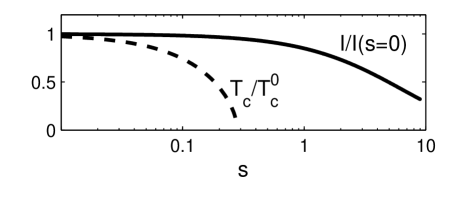
Figure 1: The $h/2e$ harmonic (full line) and $T_{c}/T_{c}^{0}$ (dashed line) as functions of the pair-breaking strength, displayed on a logarithmic scale. The current, in units of $I(s=0)$, is plotted for $T=E_{c}$ and $T_{c}^{0}=0.1E_{c}$. The PC reduction at $s=10$ corresponds to $1/\tau_{s}=\pi E_{c}$.

Figure 2 portrays the PC plotted by numerically evaluating Eq. (26). In each of the panels the upper curve is drawn for $s=0$, while the second curve corresponds to a pair-breaking strength [see Eq. (28) and Fig. 1] which is large enough to destroy $T_{c}$. Nonetheless, the PC is hardly affected as long as $L_{s}\gtrsim L$ [see Eqs. (2) and (3)]. The considerably-reduced PC due to a small $L_{s}$ is presented by the dash-dotted curves, which correspond to $L_{s}\simeq 0.5L$. The effect of the temperature on the magnitude of the PC is manifested by its dependence of the ratio $L/L_{T}$, where $L_{T}$ is the thermal length,

$$L_{T}=\sqrt{D/T}\ ,$$ (30)

or equivalently the ratio $T/E_{c}$, see Fig. 2.

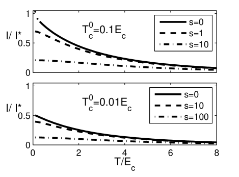
Figure 2: The amplitude of the $h/2e$ harmonic in units of $I^{*}=-eE_{c}$, as a function of the temperature, for two values of $T_{c}^{0}/E_{c}$ and several values of $s$. Note that the $s=0$ curve in the upper panel is valid only for $T/T_{c}\geq 1+Gi$, where $Gi$ is the Ginzburg parameter.

III The dominant fluctuations

Our result for the PC [see Eq. (24)] consists of infinite sums over the frequencies and over the momenta. One naturally asks oneself whether the characteristic features of the expression are not given by the first few members of each sum, notably the static, $\nu=0$, regime. It turns out that this is not the case over most of the relevant range: to obtain the correct magnitude of the fluctuation-induced PC, numerous frequencies and momenta are required.

In order to study this aspect, it is convenient to express the PC in a form which is more amenable to numerical computations. To this end we write Eq. (26) as

$$I=\frac{2ieT}{\pi}\sum_{m=1}^{\infty}\sin(4\pi m\phi)\sum_{\nu}\int_{-\infty}^{\infty}dxe^{2\pi ix}$$

$$\times\frac{d}{dx}\ln\left[\Psi(F(x,\nu))-\ln(T^{0}_{c}/4\gamma_{E}T)\right]\ ,$$ (31)

where the function $F$ is given in Eq. (27). The $x$-integration is carried out by closing the integral in the upper half of the complex plane. Two sets of simple poles can be identified in the integrand of Eq. (31). These sets result from (a) the zeros and (b) the poles of the argument of the logarithm.COM4 The first set of poles, denoted by $x^{\ell}_{\rm zero}$, is given by

$$\Psi(F^{\ell}_{\rm zero})=\ln(T^{0}_{c}/4\gamma_{E}T)\ .$$ (32)

The second set consists of the poles of the digamma function. These are denoted by $x^{\ell}_{\rm pole}$, and are obtained from the relation

$$F^{\ell}_{\rm pole}=-\ell\ ,\ \ \ell=0,1,2,\ldots\ .$$ (33)

The index $\ell$ runs over the poles in each set. The two sets of $F^{\ell}_{\rm pole/zero}$ given by Eqs. (32) and (33), are shown in Fig. 3.

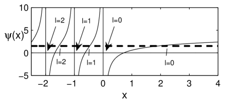
Figure 3: The digamma function (solid line) and $\ln(T^{0}_{c}/4\gamma_{E}T)$ for $T_{c}^{0}/T=0.6$ (dashed line). The first three solutions $F^{\ell}_{\rm zero}$ of Eq. (32) are marked on the x axis with their indices indicated below it. The first values of the set $F^{\ell}_{\rm pole}$, Eq. (33), are marked by arrows.

Performing the Cauchy integration, the current takes the formCOM5

$$I= -4eT\sum_{m=1}^{\infty}\sin(4\pi m\phi)$$

$$\times\sum_{\nu}\sum_{\ell=0}^{\infty}\Bigl{[}\exp(2\pi ix_{\textrm{zero}}^{\ell})-\exp(2\pi ix_{\textrm{pole}}^{\ell})\Bigr{]}\ .$$ (34)

Here $x^{\ell}_{\rm pole/zero}$ depends on the Matsubara frequency and the harmonic index $m$,

$$x_{\rm pole/zero}^{\ell}$$

$$=im\sqrt{\frac{T}{2\pi E_{c}}}\Bigl{[}1+\frac{|\nu|+2/\tau_{s}}{2\pi T}-2F_{\rm pole/zero}^{\ell}\Bigr{]}^{1/2}\ .$$ (35)

Note that all the exponents ($2\pi ix$) in the two series in Eq. (34) are negative, and their absolute value increases with increasing $\nu,l$ or $m$. As can be seen from Fig. 3, for each pair of poles $F^{\ell}_{\rm zero}>F^{\ell}_{\rm pole}$, and consequently $|x^{\ell}_{\rm zero}|<|x^{\ell}_{\rm pole}|$. This ensures that the term in the square brackets of Eq. (34) is positive, and hence the response of the ring to a small flux is diamagnetic, as it should be.

III.1 The dominant imaginary time fluctuations

The dominant terms in Eq. (34) are those for which the absolute value of $x$ is smaller than unity, but if the absolute values of all $x$ are larger than one only the smallest [$x_{\rm zero}^{\ell=0}(\nu=0,m=1)$] is the dominant one. The absolute value of the exponents (which are given by $2\pi|x_{{\rm zero}/{\rm pole}}|$) is at least $(|\nu|/E_{c})^{1/2}$. Thus, the frequencies that contribute mostly to the current are those for which $|\nu|\lesssim 10E_{c}$. The proportionality factor, of order $10$, had been determined numerically and resulted from the square-root structure of the exponents, see Eq. (35). At high temperatures $T>E_{c}$ the system is dominated by the classical fluctuations - namely, by the first (lowest energy), $\nu=0$, Matsubara frequency. The effect of the quantum fluctuations for which $\nu\neq 0$ increases as the temperature decreases. This tendency has an exception in two cases. First, for very strong pair breaking $1/\tau_{s}>\{T,E_{c},T^{2}/E_{c}\}$ the significant quantum fluctuations that have a dominant contribution to the PC are bounded by $|\nu|<\sqrt{E_{c}/\tau_{s}}$. Second, in the case of small or zero pair breaking when $T\rightarrow T_{c}$, only $\nu=0$ is the dominant frequency.LV

When $T_{c}$ is finite, the $n=\nu=0$ pole of the partition function, Eq. (7), is the most dominant one as $T\rightarrow T_{c}$. Consequently, in this low-temperature regime physical properties, including the PC, are determined only by the $\nu=0$ fluctuations, pertaining to the static Ginzburg-Landau free energy. We find however, that in the case of a vanishing $T_{c}$, quantum fluctuations, for which $\nu\neq 0$ have a significant contribution to the PC at low temperatures. Indeed, the quantum fluctuations of a system with no magnetic impurities and for which $|\phi|^{2}>T_{c}^{0}/(16\pi\gamma_{E}E_{c})$ have been recently invoked in the context of the “strong” Little-Parks oscillations, see Ref. SO, .

III.2 The dominant spatial fluctuations

High Matsubara frequencies involve many spatial frequencies ${\bf q}$. Thus, at low temperatures and for a vanishing $T_{c}$, many wave vectors contribute to the PC. We have estimated numerically their number by comparing the PC computed with a relatively small number of frequencies and wave vectors with the exact result Eq. (34) for $T=T_{c}^{0}=0.1E_{c}$ and $s=1$. In this case we have found that $\sim 100$ Matsubara frequencies are required. The highest momenta, Eq. (69), that contribute significantly are given by $|n|\sim(1,5,100,1000)$ for the frequencies $\nu/(2\pi T)=(0,5,10,100)$, respectively. Figure 4 shows the PC as computed from Eq. (24) for different maximal $|{\bf q}|$ values and without limiting the range of $\nu$. It is thus seen that in the whole range of $\phi$ the persistent current is not mainly determined by the lowest momenta, even when the size of the system $L$ is smaller than the thermal length $L_{T}$, Eq. (30). This is different than the situation in the calculations of other properties (for example, weak-localization corrections 0D to the conductivity), in which $L\ll L_{T}$ is taken as a sufficient condition for using only $q=0$. We point out however that the slope of the PC at $\phi=0$ appears to be describable using the smallest wave number only.

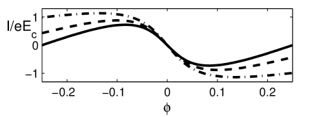
Figure 4: The PC as computed from Eq. (24), with the summation over $n$ cut at $1000,3,1$ (solid, dashed and dash-dotted curves, respectively). The plots are for $T=T_{c}^{0}=0.1E_{c}$ and $s=1$.

III.3 The dominant harmonics

Examining the series in Eq. (34) one can see that the maximal harmonic of the flux, $m_{\max}$, that has still a significant contribution to the current is given by $\min\{\sqrt{E_{c}/T},\sqrt{E_{c}\tau_{s}}\}$ or by one if the first two values are smaller than unity. This condition can be expressed in terms of lengths by

$$m_{\max}=\min\{L_{s}/L,\ L_{T}/L\}\ ,\ \textrm{ or 1}.$$ (36)

The upper limit on the harmonics results from the fact that the $m$’th harmonic is associated with paths that encircle the ring (coherently) $m$ times and hence their length is at least $mL$. Argaman The sinusoidal shape $I\propto\sin(4\pi\phi)$ at high temperatures is modified due to higher harmonics as the temperature decreases. In the absence of magnetic impurities (upper panel in Fig. 5) the low-temperature current as a function of the flux attains a sawtooth shape. Such a behavior is predicted also for the equilibrium PC in superconductors at zero temperature book and for the persistent current in a clean system of non-interacting electrons.Cheung_Gefen_Riedel_Shih_1988 In the presence of pair-breakers the upper bound on the harmonics Eq. (36) prevents the current from reaching the sharp sawtooth shape. This suggests, in principle, a way to experimentally confirm the role of pair breaking for this problem. In the lower panel of Fig. 5 the current of a system with $L\simeq L_{s}$ is plotted for several temperatures. At temperatures below $0.1E_{c}$ the shape of the current does not change anymore.

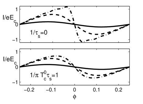
Figure 5: The current, in units of $eE_{c}$, as a function of the flux $\phi$, for $T_{c}^{0}/E_{c}=0.1\;$ and for several temperatures, $T/E_{c}=5,1$ and $0.15$ in the solid, dashed and dash-dotted curves respectively. In the lower panel the dash-dotted curve corresponds to $T/E_{c}=0.1$. For $s=0$ the current attains the sawtooth form (upper panel) which is lost for $s=1$ (lower panel).

IV The temperature dependence

Here we study the PC in the low and high-temperature regimes. In particular we find that the PC decays exponentially as the length of the ring exceeds the thermal length $L_{T}$ or the magnetic impurity scattering length $L_{s}$, whichever is shorter.

IV.1 High-temperature regime, $T\gg\max\{1/\tau_{s},T_{c}^{0},E_{c}\}$

When the temperature is much higher than all relevant energy scales, i.e., $T\gg\max\{1/\tau_{s},T_{c}^{0},E_{c}\}$, the leading contribution to the double sum in Eq. (34) comes solely from the first pole $x^{\ell=0}_{\rm zero}$ of the lowest Matsubara frequency, $\nu=0$ [see Eq. (35)]. In this temperature range the $h/2e$ harmonic, corresponding to $m=1$, is the dominant one.

As the temperature increases, the horizontal line in Fig. 3 representing $\ln(T_{c}^{0}/4\gamma_{E}T)$ moves further down, so that $F_{\textrm{zero}}^{\ell=0}$ approaches zero. We use the expansion of the digamma function for small arguments in Eq. (32) and obtain

$$F_{\textrm{zero}}^{\ell=0}=\left[\ln(T_{c}^{0}/4\gamma_{E}^{2}T)\right]^{-1}\ .$$ (37)

Upon substituting this result in the dominant term of Eq. (34), we obtain the current in the form

$$I\simeq-4eT\sin(4\pi\phi)$$

$$\times\exp\Bigl{(}-\frac{L}{L_{T}}\Bigl{[}2\pi+\frac{2L^{2}_{T}}{L^{2}_{s}}-\frac{4}{\pi\ln(4\gamma_{E}^{2}T/T_{c}^{0})}\Bigr{]}^{1/2}\Bigr{)}\ .$$ (38)

We compare the full result, Eq. (34), with the high-temperature approximation Eq. (38) in Fig. 6. The difference between the contributions of the first $x^{\ell=0}_{\rm zero}(\nu=0)$ and the second $x^{\ell=0}_{\rm pole}(\nu=0)$ poles to the PC is the absence of the third term, which includes a logarithm [see Eq. (38)], in the exponent of the latter. Therefore, this approximation improves as $T_{c}^{0}$ increases.

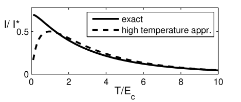
Figure 6: The amplitude of the $h/2e$ harmonic is plotted in units of $I^{*}=-eE_{c}$ as a function of the temperature, for $T_{c}^{0}/E_{c}=0.1$ and $s=1$. The exact results can be approximated by Eq. (38) for $T\gg E_{c}$.

IV.2 Low-temperature regime, $T_{c}\ll T\ll\{1/\tau_{s},E_{c}\}$

In the low temperature regime the argument ($F$) of the digamma function and its derivative is much larger than unity [see Eq. (27)], so that we can use their asymptotic expansions $\ln(F)$ and $1/F$, respectively. Substituting these approximations in Eq. (26) gives

$$I=-\frac{8}{\pi}\;eT\sum_{m=1}^{\infty}\sin(4\pi m\phi)$$

$$\times\sum_{\nu}\int_{0}^{\infty}\frac{x\sin(2\pi x)dx}{\ln\left[\frac{4\pi\gamma_{E}E_{c}}{T_{c}^{0}}(x^{2}+a_{m,\nu})\right](x^{2}+a_{m,\nu})}\ ,$$ (39)

where $a_{m,\nu}=m^{2}(|\nu|+2/\tau_{s}+2\pi T)/(4\pi^{2}E_{c})$. For $T\gg T_{c}$ the denominator in Eq. (39) does not vanish. Then the term $x^{2}+a_{m,\nu}$ in the logarithm in Eq. (39) can be replaced by $\alpha a_{m,\nu}$, with, say, $1<\alpha<3$. Consequently,

$$I\simeq -4eT\sum_{m}\sin(4\pi m\phi)\sum_{\nu}e^{-m\sqrt{\frac{2\pi T}{E_{c}}}\sqrt{1+\frac{|\nu|+2/\tau_{s}}{2\pi T}}}$$

$$/\ln\left[\frac{2\gamma_{E}\alpha T}{T_{c}^{0}}\left(1+\frac{|\nu|+2/\tau_{s}}{2\pi T}\right)\right]\ .$$ (40)

Since $T\ll E_{c}$ the summation over $\nu$ can be replaced by an integration. Approximating again the logarithm by its value at the dominant $\nu$ of the integration, yields

$$I\simeq -\frac{8}{\pi}\;eE_{c}\sum_{m}\frac{\sin(4\pi m\phi)}{m^{2}}\left[1+m\sqrt{\frac{2\pi L^{2}}{L_{T}^{2}}+\frac{2L^{2}}{L_{s}^{2}}}\right]$$

$$\times e^{-m\sqrt{\frac{2\pi L^{2}}{L_{T}^{2}}+\frac{2L^{2}}{L_{s}^{2}}}}/\ln\left[\frac{\gamma_{E}\alpha E_{c}}{\pi T_{c}^{0}m^{2}}\bar{z}\right]\ ,$$ (41)

where $\bar{z}=\max\{1,2m^{2}/\tau_{s}E_{c}\}$.

We compare in Fig. 7 the low-temperature approximation, Eq. (IV.2), with the full result, Eq. (34). As one can see from this comparison, the flux dependence of the PC as well as its amplitude are well approximated by Eq. (IV.2).

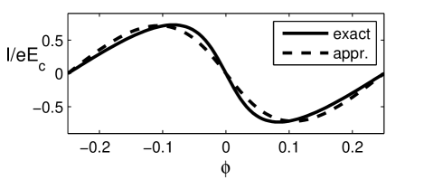
Figure 7: The current in units of $eE_{c}$ as a function of the magnetic flux $\phi$, plotted for $T=0.1T_{c}^{0}=0.01E_{c}$ and $s=1$. The low-temperature approximation Eq. (IV.2) is compared with the exact result Eq. (34). We take $\alpha=3$ in the logarithm of Eq. (IV.2).

V Renormalization of the effective interaction

In this section we calculate the PC to first order in the interaction, in order to see whether it suffices to explain our full result. To first order in the interaction, the contribution of superconducting fluctuations to the free energy [see Eq. (7)] is

$$\Delta\Omega=-(gT^{2}/V)\sum_{{\bf q},\nu}\Pi({\bf q},\nu)\ .$$ (42)

The PC resulting from Eq. (42) has the same form as Eq. (24), except that the denominator in the latter is replaced by the bare interaction $g{\cal N}(0)/V$. Had we tried to to fit the experimental data of Refs. LDDB, and JMKW, using Eq. (42), we should have taken the implausible ratio $E_{c}\sim 0.1\omega_{D}$ [see Eq. (20)]. This first-order approximation fails because of screening effects, which increase the magnitude of the effective attractive interaction as the temperature decreases. Very roughly, the renormalization of a dimensionless interaction $\lambda$, from a higher frequency scale $\omega_{>}$ to a lower one, $\omega_{<}$, is given byMA

$$\lambda(\omega_{<})=\left[\lambda^{-1}(\omega_{>})-\ln\left(\frac{\omega_{>}}{\omega_{<}}\right)\right]^{-1}\ .$$ (43)

For attractive interactions $\lambda$ is positive and the high frequency scale is $\omega_{D}$. At $T=T^{0}_{c}$ and $1/\tau_{s}=0$, the attractive interaction should diverge. Using this to eliminate $\lambda(\omega_{D}$) ($\equiv g{\cal N}(0)/V$), we obtain that for $T^{0}_{c}\lesssim\omega\ll\omega_{D},$

$$\lambda(\omega)\backsim 1/\ln(\omega/T_{c}^{0})\ .$$ (44)

Replacing in the first-order approximation for the current the bare interaction by the effective one, Eq. (44), gives

$$I_{\textrm{1st}}=-\frac{8eE_{c}}{\ln(\omega/T_{c}^{0})}\sum_{m=1}^{\infty}\frac{\sin(4\pi m\phi)}{m^{2}}$$

$$\times\sum_{\nu}\int_{0}^{\infty}dxx\sin(2\pi x)\Psi^{\prime}(F(x,\nu))\ .$$ (45)

The effective interaction is renormalized upwards with decreasing energy and, for the bulk and no pair breaking, it blows up at $T_{c}^{0}$. For $1/\tau_{s}>T_{c}^{0}$, this renormalization stops at $1/\tau_{s}$ and $T_{c}$ disappears. In the mesoscopic range, the Thouless energy, $E_{c}$, becomes a relevant scale and it may be expected (as is borne out by our results) that the PC at low temperatures is determined by the interaction on that scale, as long as $E_{c}\gtrsim 1/\tau_{s}$. Once $1/\tau_{s}\gtrsim E_{c}$, we expect the renormalization to “stop at $1/\tau_{s}$” and the PC to be depressed. Thus, the relevant range for our considerations is $T_{c}^{0}\lesssim 1/\tau_{s}\lesssim E_{c}$. Using these bounds on the energy scale of the renormalized interaction in the first order calculation Eq. (V), gives a good agreement with our result Eq. (34). In Fig. 8 we plot the amplitude of the $h/2e$ harmonic as a function of $T/E_{c}$, calculated from the full expression Eq. (26) (thin curves) and from the first-order approximation Eq. (V) (bold curves).

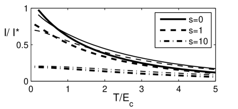
Figure 8: The first-order approximation for the $h/2e$ harmonic of the current Eq. (V) (bold lines) is compared with the exact result (thin lines). Here $T_{c}^{0}=0.1E_{c}$. In drawing the former, we have used the simplest expression for the cutoff $\omega=T+E_{c}+1/\tau_{s}$ .

The plotted curves are for $T_{c}^{0}=0.1E_{c}$.

A more precise expression for the renormalized attractive interaction depends on ${\bf q},\nu$ of the order-parameter fluctuation. The renormalized attractive interaction $\lambda({\bf q},\nu)$, obtained from an infinite series of diagrams containing Cooperon contributions, is given by AA

$$\lambda({\bf q},\nu)=\Big{[}\lambda^{-1}(\omega_{D})-\frac{T}{{\cal N}(0)}\Pi({\bf q},\nu)\Big{]}^{-1}\ .$$ (46)

Upon substituting Eq. (II) in Eq. (46) one can identify $\lambda({\bf q},\nu)$ from our result, e.g., by comparing Eq. (V) with Eq. (24).

VI Comparison with experiments

Theoretically, only static magnetic fields have been considered here. However, experiments have been carried out with an ac magnetic field. In the experiments on copperLDDB and gold,JMKW the sweeping frequencies of the magnetic field were very low ($0.3$ Hz and $2$Hz respectively). Thus, one expects that the measured PC could be explained using a theory for a static magnetic field. In the experiment on silver, on the other hand, a very high sweeping frequency of the magnetic field was used ($217$ MHz). It is plausible that in order to explain the results of Ref. DBRBM, one may not confine oneself to a static magnetic field. We therefore do not attempt to explain the experiment of Ref. DBRBM, .

Here we explain the $h/2e$ signal observed in copperLDDB and goldJMKW using our result Eq. (34). In the left six columns of Table 1 we summarize the experimental parameters for the $(h/2e)$-periodic signal.COM6

	$E_{c}$	$T$	$I/eE_{c}$	$L$	$L_{\varphi}$	min $T_{c}^{0}$
CopperLDDB	$15$ mK	$7$ mK	$1$	$2.2\;\mu$m	$2\;\mu\textrm{m}(1.5\textrm{ K})$	a few mK
GoldJMKW	$4.9$ mK	$5.5$ mK	$0.65$	$8.0\;\mu$m	$16\;\mu\textrm{m}(0.5\textrm{ K})$	a fraction of a mK

Table 1: Experimental parameters in the left six columns. The magnitude of the $h/2e$ periodic current (column $4$) is given for the lowest temperature (column $3$) reached in the experiment. The dephasing length $L_{\varphi}$ is given together with the temperature at which it was measured. The last column is our estimate for a lower bound on $T_{c}^{0}$ according to Eq. (34), see also Fig. 9.

The metals used in the experiments are not superconductors at any measured temperature in their bulk form. Therefore, it is not possible to obtain theoretically a large enough PC (to match the measurmentsLDDB ; JMKW ) due to the attractive interaction without pair breaking: the required $T_{c}\sim 1$ mK are too high to be considered as realistic. We suggest that the bare transition temperature may indeed be of the order of a mK, but the transition temperature of the real material is considerably reduced due to pair breakers. Together with this assumption, the necessary condition to fit the experiments is $1/\tau_{s}\gtrsim\pi T_{c}^{0}/2\gamma_{E}$ so that $T_{c}$ vanishes or is very strongly depressed,AG see Eq. (28). This condition can also be written as

$$\frac{T_{c}^{0}}{E_{c}}\lesssim\frac{2\gamma_{E}}{\pi}\left(\frac{L}{L_{s}}\right)^{2}\ .$$ (47)

Note that we need $L_{s}\gtrsim L$ in order not to depress the PC [Eq. (34)]. The upper limit on $T_{c}^{0}$, corresponding to the equality in Eq. (47), is given by the solid line in Fig. 9. The values for $T_{c}^{0}/E_{c}$ that correspond to a vanishing $T_{c}$ are in the region below this line. In the dashed and dash-dotted curves in Fig. 9 different values of $L/L_{s}$ are matched with an appropriate $T_{c}^{0}/E_{c}$ so that the measured values in columns $2-4$ of Table 1 remain the same.

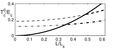
Figure 9: The bare transition temperatures corresponding to the measured PC as a function of $L/L_{s}$. The dashed and dash-dotted curves correspond to the PC measured in copper and gold, respectively. The solid curve gives the maximal possible $T_{c}^{0}$ satisfying $T_{c}=0$.

The monotonically increasing shape of the curves in Fig. 9 results from the fact that higher values of $T_{c}^{0}/E_{c}$ are required to describe the experiments as $L/L_{s}$ increases. The minimal $T_{c}^{0}$’s correspond to the points where the dashed and the dash-dotted lines cross the solid line. In this way we obtain estimates of the lower bounds on the value of $T_{c}^{0}$ for copper and gold. These lower bounds are given in the seventh column of Table 1.

These estimates of $T_{c}^{0}$ are very sensitive [see Eqs. (IV.2) and (V)] to the experimental parameters. For example, Ref. LDDB, points out that the measured values of the PC are correct up to a factor of two. The exact minimal value of $T_{c}^{0}$ that satisfies Eq. (47) for copper, based on the values quoted in Table 1, is $4$mK. However, assuming half of the value reported in Ref. LDDB, for the PC, results in a minimal $T_{c}^{0}$ of about $0.3$mK. The curves in Fig. 9 ignore the error bars in the experiments. Thus, the values of $T_{c}^{0}/E_{c}$ in this figure should be considered only as rough estimates.

Besides spin-flip scattering from magnetic impurities, decoherence of the electrons is also caused by other processes, e.g., electron-phonon inelastic interactions. Hence $L_{s}$ is always larger or of the order of the dephasing length. A lower bound on $L_{s}$ is given by equating it to the measured $L_{\varphi}$. Those values (see Table 1) are small enough to fulfil the condition in Eq. (47). In other words, we could account for the data of copper and gold since the measured $L_{\varphi}$ was small enough. This is not the case for silver, DBRBM where $L/L_{\varphi}(=0.3)$ is too small to explain the result $I(T=4.6E_{c})=1.6eE_{c}$ using Eq. (34). Our theory is not applicable to that experiment. We believe that the reason for that, as explained above, is the high frequency used in that experiment.

VII Discussion

In our result for the PC, Eq. (34), there appears the bare transition temperature and not the one reduced by the pair-breaking mechanism. Therefore we propose the scenario, in which the bulk transition temperature vanishes due to the pair-breaking mechanism, while the PC is dominated by a relatively high attractive interaction.

The bulk $T_{c}$ vanishes due to pair breaking for $L_{s}<\xi(0)$. However, we find that the PC may still be hardly affected by pair breaking. The physical reason for that is that as long as $L_{s}>L$ the Cooper pair fluctuations can complete a circle around the ring before being magnetically scattered, and hence respond to the Aharonov-Bohm flux. The PC is immune to pair breaking in the regime given by Eq. (2) where the bulk form is normal. This is demonstrated in Figs. 1 and 2.

In the pair-breaking regime given by Eq. (2), the upper bound on the dominant quantum fluctuations ($\nu\neq 0$) is determined by the Thouless energy. Dominant fluctuations of high Matsubara frequencies necessitate high wave numbers. Therefore, at low temperature $T\ll E_{c}$ high wave numbers are involved too in the dominant fluctuations [see Fig. 4], in contrast to the effective dimensional reduction occurring in other phenomena when $L\ll L_{T}$, notably weak-localization corrections.0D The maximal number of flux harmonics that contribute to the PC, Eq. (36), is bounded due to thermal fluctuations and due to spin-flip scattering. Consequently, in a system with magnetic impurities, even at zero temperature the PC may not have the sawtooth shape, which appears for the PC’s without pair breaking, see Fig. 5.

The effective interaction is renormalized upwards with decreasing energy; For the bulk it stops at $\sim\max\{T_{c}^{0},1/\tau_{s}\}$ (which explains why $T_{c}$ disappears for $1/\tau_{s}\gtrsim T_{c}^{0}$). In the mesoscopic range, $E_{c}\gtrsim T_{c}^{0}$, the Thouless energy sets another bound for the energy scale at which the renormalization stops. In Sec. V it is shown that these considerations agree with our result for the PC Eq. (34), see Fig. 8.

We found that in the high-temperature regime, the PC decreases exponentially with $L/L_{s}$ or with $L/L_{T}$, whichever is larger. The explicit exponential decay of the PC with $L/L_{s}$ in both the high and the low temperature regimes [Eqs. (38) and (IV.2) respectively] for $L\gtrsim L_{s}$ is in agreement with the qualitative argument of Eq. (2). Note that Eq. (IV.2) is applicable only at very low temperatures, such that $T\ll\{T_{c}^{0},E_{c}\}$. The experiments on copperLDDB and goldJMKW rings correspond to $T_{c}^{0}\sim 1mK$, thus Eq. (IV.2) can be used only at very low temperatures $T\ll 1mK$. In the experiments the lowest temperature was $\sim 10$ mK, and therefore the measured PC cannot be precisely fitted by the approximate expression Eq. (IV.2). In the low-temperature regime the dependence of the PC on $T_{c}^{0}$ is logarithmically weak [see Eq. (IV.2)]. This weak dependence explains why in Ref. AEEPL, , where the transition temperature was taken as $10\mu$K (in the absence of pair breaking), the result was smaller only by a factor of $\sim 5$ compared with the experiment.LDDB

Interestingly enough, it follows from our work that by measuring the PC and the pair-breaking strength one may determine $T_{c}^{0}$, which would be directly measurable only if enough low-temperature pair breaking could be eliminated. This elimination is very hard to achieve in some materials. Our result Eq. (26) can explain the large PC of Refs. LDDB, and JMKW, , with $L_{s}$ value larger than (or of the order of) the measured $L_{\varphi}$ (see Table 1 and Fig. 9). Even though $L_{s}$ was not measured in the PC experiments, we obtain a lower bound on the bare transition temperatures for copper and gold. These minimal $T_{c}^{0}$’s correspond to minimal pair-breaking strength given by $L_{s}\sim 5\;\mu$m in the copper sampleLDDB and $L_{s}\sim 25\;\mu$m in the gold sample.JMKW The fitted maximal $L_{s}$’s can be caused by a very low (less than one part per million) concentration of magnetic impurities. These concentrations seem appropriate for the purest copper and gold samples available experimentally.PGAPEB Although, a full consideration of the effect of the magnetic impurities, including Kondo physics, is still necessary.

Our result concerning the fundamentally different sensitivities of $T_{c}$ and PC’s to pair breaking is valid regardless of the situation in specific materials. Our idea can be tested, for example, by measuring the persistent currents in very small rings made of a superconducting material whose transition temperature is known, as functions of possible pair-breaking mechanisms. For $E_{c}\gtrsim 100\;$mK, say, and a material with $T_{c}^{0}$ of a few $10\;$mK, the range of pair breaking which satisfies Eq. (1) becomes easier to control experimentally.

Appendix A Derivation of the partition function

Here we derive, using the method of Feynman path integral, the partition function, Eq. (7). In terms of the Grassmann variables $\psi_{\alpha}({\bf r},\tau)$ [$\bar{\psi}_{\alpha}({\bf r},\tau)$], the partition function reads

$$\mathcal{Z}=\int D(\psi({\bf r},\tau),\bar{\psi}({\bf r},\tau))\exp(-\tilde{\cal S})\ ,$$ (48)

where the action $\tilde{\cal S}$ is

$$\tilde{\cal S}=\int d{\bf r}\int_{0}^{\beta}d\tau\left[\bar{\psi}_{\sigma}({\bf r},\tau)\partial_{\tau}\psi_{\sigma}({\bf r},\tau)+\mathcal{H}({\bf r},\tau)\right]\ .$$ (49)

Here $\beta=1/T$ and $\mathcal{H}$ is given by the integrand of the Hamiltonian, Eq. (4), with Grassmann variables (of the same imaginary time) replacing the creation and annihilation operators. Introducing the bosonic fields $\Delta({\bf r},\tau)$ via the Hubbard-Stratonovich transformation, the partition function takes the form

$$\mathcal{Z}=\int D(\psi({\bf r},\tau),\bar{\psi}({\bf r},\tau))D(\Delta({\bf r},\tau),\Delta^{\ast}({\bf r},\tau))$$

$$\times\exp(-{\cal S})\ ,$$ (50)

where the differential of the bosonic field $\Delta({\bf r},\tau)$, $D(\Delta({\bf r},\tau),\Delta^{\ast}({\bf r},\tau))$, contains a factor of $\beta V/\pi g$. The action ${\cal S}$ is given by

$${\cal S} =\int d{\bf r}\int_{0}^{\beta}d\tau\Bigl{(}\frac{|\Delta({\bf r},\tau)|^{2}}{g}$$

$$-\frac{1}{2}\bar{\Psi}({\bf r},\tau)G^{-1}_{{\bf r},{\bf r};\tau,\tau}\Psi({\bf r},\tau)\Bigr{)}\ ,$$ (51)

where $\bar{\Psi}=(\bar{\psi}_{\uparrow},\bar{\psi}_{\downarrow},\psi_{\uparrow},\psi_{\downarrow})$, and the inverse Green function $G^{-1}$ (at equal positions ${\bf r}$ and equal imaginary times $\tau$) is

$$G^{-1}_{{\bf r}={\bf r}^{\prime};\tau=\tau^{\prime}}=\left[\begin{array}[]{cccc}-\partial_{\tau}-h^{\phi}_{\uparrow}&-2u_{2}S_{-}&0&\Delta\\ -2u_{2}S_{+}&-\partial_{\tau}-h^{\phi}_{\downarrow}&-\Delta&0\\ 0&-\Delta^{\ast}&-\partial_{\tau}+h^{-\phi}_{\uparrow}&2u_{2}S_{+}\\ \Delta^{\ast}&0&2u_{2}S_{-}&-\partial_{\tau}+h^{-\phi}_{\downarrow}\end{array}\right]\equiv\left[\begin{array}[]{cccc}\hat{G}^{-1}_{\rm p}&&&\hat{\Delta}\\ &&&\\ &&&\\ \hat{\Delta}^{\dagger}&&&\hat{G}^{-1}_{\rm h}\end{array}\right]\ .$$ (60)

Here $h_{\alpha}^{\pm\phi}={\cal H}_{0}(\pm\phi)+u_{1}+{\rm sgn}(\alpha)S_{z}u_{2}$, and $S_{\pm}=(S_{x}\pm iS_{y})/2$, where ${\rm sgn}(\uparrow)=1$ and ${\rm sgn}(\downarrow)=-1$.

The integration over the fermionic part in Eq. (A) yields

$${\cal Z}=\int D(\Delta({\bf r},\tau),\Delta^{\ast}({\bf r},\tau))\exp\Bigl{(}\frac{1}{2}{\rm Tr}\ln(\beta G^{-1})-\int d{\bf r}\int_{0}^{\beta}d\tau\frac{|\Delta({\bf r},\tau)|^{2}}{g}\Bigr{)}\ .$$ (61)

We expand ${\rm Tr}\ln(\beta G^{-1})$ up to second orderCOM3 in $\Delta$

$${\rm Tr}\ln(\beta G^{-1})={\rm Tr}\ln(\beta G^{-1}_{0})-\frac{1}{(\beta V)^{2}}\iiiint d{\bf r}d{\bf r}^{\prime}d\tau d\tau^{\prime}\;{\rm Tr}\left[\hat{G}_{p}({\bf r}^{\prime},\tau^{\prime};{\bf r},\tau)\hat{\Delta}({\bf r},\tau)\hat{G}_{h}({\bf r},\tau;{\bf r}^{\prime},\tau^{\prime})\hat{\Delta}^{\dagger}({\bf r}^{\prime},\tau^{\prime})\right]\ .$$ (62)

The inverse Green function for non-interacting electrons, $G^{-1}_{0}$, is given by Eq. (60) for $\Delta=0$. The first term on the right hand side of Eq. (62), which is zeroth-order in $\Delta$, gives rise to the partition function of non-interacting electrons, ${\cal Z}_{0}=\det(\beta G^{-1}_{0})$.

In Eq. (62), $G_{p}$ ($G_{h}$) is the particle (hole) Green function. These functions are the solutions of

$$\hat{G}^{-1}_{p/h}({\bf r},\tau)\hat{G}_{p/h}({\bf r},\tau;{\bf r}^{\prime},\tau^{\prime})=\delta({\bf r}-{\bf r}^{\prime})\delta(\tau-\tau^{\prime})\ ,$$ (63)

where $G_{p/h}^{-1}$ are defined in Eq. (60). As can be seen in that equation, the particle and the hole inverse Green functions are related to one another by

$$\hat{G}^{-1}_{h}({\bf r},\tau,\phi,S_{+},S_{-},S_{z})$$

$$=-\hat{G}_{p}^{-1}({\bf r},-\tau,-\phi,S_{-},S_{+},S_{z})\ .$$ (64)

Therefore,

$$\hat{G}_{h}({\bf r},\tau;{\bf r}^{\prime},\tau^{\prime},\phi,S_{+},S_{-},S_{z})$$

$$=-\hat{G}_{p}({\bf r},-\tau;{\bf r}^{\prime},-\tau^{\prime},-\phi,S_{-},S_{+},S_{z})$$

$$=-\hat{G}_{p}({\bf r},\tau^{\prime};{\bf r}^{\prime},\tau,-\phi,S_{-},S_{+},S_{z})\ ,$$ (65)

where in the last equality we have used time-translational invariance to shift $\tau$ and $\tau^{\prime}$ by $\tau+\tau^{\prime}$. Reversing the sign of the flux $\phi$ together with interchanging ${\bf r}$ and ${\bf r}^{\prime}$ leads to the relation (the superscript $t$ denotes the transposed matrix)

$$\hat{G}_{p}({\bf r},\tau^{\prime};{\bf r}^{\prime},\tau,-\phi,S_{-},S_{+},S_{z})$$

$$=\hat{G}_{p}^{t}({\bf r}^{\prime},\tau^{\prime};{\bf r},\tau,\phi,S_{+},S_{-},S_{z})\ .$$ (66)

We have used Eqs. (65) and (66) to replace the hole Green function in Eq. (62) by a particle Green function. Then, in momentum representation, the second term of the right hand side of Eq. (62) readsCOM2

$${\rm Tr}\ln(\beta G^{-1})\Big{|}^{2\textrm{nd}}=\sum_{{\bf q}_{1},{\bf q}_{2},\nu}\sum_{{\bf k}_{1},{\bf k}_{2},\omega}{\rm Tr}\left[\hat{G}_{\rm p}({\bf k}_{1}+{\bf q}_{1},{\bf k}_{2}+{\bf q}_{2},\omega+\nu)\hat{\Delta}({\bf q}_{2},\nu)\hat{G}_{\rm p}^{t}(-{\bf k}_{1},-{\bf k}_{2},-\omega)\hat{\Delta}^{\dagger}({\bf q}_{1},\nu)\right]\ .$$ (67)

The flux dependence is incorporated into the momenta ${\bf p}$, where ${\bf p}^{2}/2m-\mu$ are the eigenvalues of ${\cal H}_{0}(\phi)$. Thus, the longitudinal components of the momenta in the Green function $G$ have the form

$$2\pi(n+\phi)/L\ ,$$ (68)

while those of the momenta in the boson field $\Delta$ are

$$2\pi(n+2\phi)/L\;,$$ (69)

where $n$ is an integer. The Matsubara frequencies of the Green functions, $\omega+\nu$ and $-\omega$, are fermionic $[=\pi(2n+1)T]$. The order-parameter fluctuations are characterized by the Matsubara bosonic frequencies $\nu=2\pi nT$.

The resulting expression for the partition function may be simplified since the terms that survive the disorder-average in the sum of Eq. (67) are those for which AGD ${\bf q}_{1}={\bf q}_{2}$. Following Ref. AGD, , we disorder-average over the exponent in Eq. (61), rather than over the free energy, to obtain an answer which is correct to leading order in $(\mu\tau_{+})^{-1}$. Finally we trace over the product of the $2\times 2$ matrices in Eq. (67) and integrate over $\Delta$ in Eq. (61). In this way we obtain the partition function, Eq. (7).

References

- (1) L. Gunther and Y. Imry, Solid State Commun. 7, 1391 (1969); M. Büttiker, Y. Imry, and R. Landauer, Phys. Lett. 96A, 365 (1983).
- (2) Y. Imry, Introduction to Mesoscopic Physics, 2nd ed (Oxford University Press, Oxford, 2002).
- (3) L. P. Levy, G. Dolan, J. Dunsmuir, and H. Bouchiat, Phys. Rev. Lett. 64, 2074 (1990).
- (4) R. Deblock, R. Bel, B. Reulet, H. Bouchiat, and D. Mailly, Phys. Rev. Lett. 89, 206803 (2002).
- (5) V. Chandrasekhar, R. A. Webb, M. J. Brady, M. B. Ketchen, W. J. Gallagher, and A. Kleinsasser, Phys. Rev. Lett. 67, 3578 (1991).
- (6) H. Bluhm, N. C. Koshnick, J. A. Bert, M. E. Huber, and K. A. Moler, Phys. Rev. Lett. 102, 136802 (2009).
- (7) E. M. Q. Jariwala, P. Mohanty, M. B. Ketchen, and R. A. Webb, Phys. Rev. Lett. 86, 1594 (2001).
- (8) H. F. Cheung, E. K. Riedel, and Y. Gefen, Phys. Rev. Lett. 62, 587 (1989); E. K. Riedel and F. von Oppen, Phys. Rev. B 47, 15449 (1993); O. Entin-Wohlman and Y. Gefen, Europhys. Lett. 8, 477 (1989). These results and their extensions will be discussed in a forthcoming publication by the present authors.
- (9) B. L. Altshuler, Y. Gefen, and Y. Imry, Phys. Rev. Lett. 66, 88 (1991).
- (10) V. Ambegaokar and U. Eckern, Europhys. Lett. 13, 733 (1990).
- (11) V. Ambegaokar and U. Eckern, Phys. Rev. Lett. 65, 381 (1990).
- (12) D. Mailly, C. Chapelier, and A. Benoit, Phys. Rev. Lett. 70, 2020 (1993).
- (13) B. Reulet, M. Ramin, H. Bouchiat, and D. Mailly, Phys. Rev. Lett. 75, 124 (1995); R. Deblock, Y. Noat, B. Reulet, H. Bouchiat, and D. Mailly, Phys. Rev. B 65, 075301 (2002).
- (14) See note added in proof in Ref. AEPRL, .
- (15) P. G. de Gennes, Superconductivity of Metals and Alloys (Addison-Wesley Publishing Co., 1989).
- (16) P. Morel and P. W. Anderson, Phys. Rev. 125, 1263 (1962); N. N. Bogoliubov, V. V. Tolmachev, and D. V. Shirkov, A New Method in the Theory of Superconductivity (Consultants Bureau, Inc., New York, 1959).
- (17) The fluctuation correction to the orbital magnetic response above was calculated first by L. G. Aslamazov and A. I. Larkin, Sov. Phys. JETP 40, 321 (1975).
- (18) The of the noble metals were estimated using varying amounts of alloying by R. F. Hoyt and A. C. Mota, Solid State Commun. 18, 139 (1976). The pair-breaking strengths in these alloys are not precisely known.
- (19) F. Pierre, A. B. Gougam, A. Anthore, H. Pothier, D. Esteve, and N. O. Birge, Phys. Rev. B 68, 085413 (2003).
- (20) B. L. Altshuler, A. G. Aronov, and D. E. Khmelnitskii, J. Phys. C 15, 7367 (1982).
- (21) A. A. Abrikosov and L. P. Gorkov, Soviet Physics JETP 12, 1243 (1961).
- (22) Y. Imry, H. Fukuyama, and P. Schwab, Europhys. Lett. 47, 608 (1999).
- (23) P. A. Lee and N. Read, Phys. Rev. Lett. 58, 2691 (1987).
- (24) G. Schwiete and Y. Oreg, cond-mat/0812.4088 (2008). These results are relevant to recent experiments in Al rings, see N. C. Koshnick, H. Bluhm, M. E. Huber, and K. A. Moler, Science 318, 1440 (2007).
- (25) U. Eckern and P. Schwab, J. Low Temp. Phys. 126, 1291 (2002).
- (26) V. E. Kravtsov and B. L. Altshuler, Phys. Rev. Lett. 84, 3394 (2000).
- (27) A. Altland and B. Simons, Condensed Matter Field Theory (Cambridge University Press, Cambridge, 2006).
- (28) H. Bary-Soroker, O. Entin-Wohlman, and Y. Imry, Phys. Rev. Lett. 101, 057001 (2008).
- (29) This expansion, up to second order in , is valid for temperatures well above the transition temperature, and, strictly speaking, above the Ginzburg critical region. In the case of interest to us, in which vanishes, it is not obvious that a finite Ginzburg critical region exists at all.
- (30) The order of the momenta of the second Green function has been interchanged in Eqs. (9) and (12) of Ref. BarySoroker_EntinWohlman_Imry, . This typo was not carried on in the derivation there.
- (31) A. A. Abrikosov, L. P. Gorkov, and I. E. Dzyaloshinski, Methods of Quantum Field Theory in Statistical Physics (Prentice-Hall, Englewood Cliffs, NJ, 1963).
- (32) B. L. Altshuler and A. G. Aronov, in Electron-electron interactions in disordered systems, edited by A. L. Efros and M. Pollak (North-Holland, Amsterdam, 1985).
- (33) Equation (28) generalizes the result of Ref. AG, to include the effect of a finite flux.
-
(34)
We use the fact that any meromorphic function can be written
locally as , where . Hence,
where has a simple pole at with a residue .(70) - (35) The difference in sign between the zero and the pole terms in Eq. (34) is due to the different sign of in Eq. (70) for the poles and the zeros of the function in the logarithmic derivative. [We checked numerically that Eq. (26) and Eq. (34) are identical.]
- (36) A. Larkin and A. Varlamov, Theory of Fluctuation in Superconductors (Clarendon press, Oxford, 2005).
- (37) B. L. Altshuler, A. G. Aronov, D. E. Khmelnitskii, and A. I. Larkin, in Quantum theory of solids, edited by I. M. Lifshits (MIR, Moscow, 1983), section 3.2.4.
- (38) N. Argaman, Y. Imry, and U. Smilansky, Phys. Rev. B 47, 4440 (1993).
- (39) H. F. Cheung, Y. Gefen, E. K. Riedel and W. H. Shih, Phys. Rev. B 37, 6050 (1988).
- (40) Prefactors in the definition of the Thouless energy vary in the literature.