Abstract

The Lorentz transformations of electric and magnetic fields were implemented to study (i) the refraction of linearly polarized plane waves into a half–space occupied by a uniformly moving material, and (ii) the traversal of linearly polarized Gaussian beams through a uniformly moving slab. Motion was taken to occur tangentially to the interface(s) and in the plane of incidence. The moving materials were assumed to be isotropic, homogeneous, dissipative dielectric materials from the perspective of a co–moving observer. Two different moving materials were considered: from the perspective of a co–moving observer, material A supports planewave propagation with only positive phase velocity, whereas material B supports planewave propagation with both positive and negative phase velocity, depending on the polarization state. For both materials A and B, the sense of the phase velocity and whether or not counterposition occurred, as perceived by a nonco–moving observer, could be altered by varying the observer’s velocity. Furthermore, the lateral position of a beam upon propagating through a uniformly moving slab made of material A, as perceived by a nonco–moving observer, could be controlled by varying the observer’s velocity. In particular, at certain velocities, the transmitted beam emerged from the slab laterally displaced in the direction opposite to the direction of incident beam. The transmittances of a uniformly moving slab made of material B were very small and the energy density of the transmitted beam was largely concentrated in the direction normal to the slab, regardless of the observer’s velocity.

PACS numbers: 03.30.+p, 03.50.De, 41.20.Jb

1 Introduction

What happens to plane waves at the planar interface of two passive linear mediums is one of the staple problems of electrodynamics. Relative motion between the two mediums on either side of the interface can give rise to complex electromagnetic behaviour — exemplified by materials which support negative refraction [1] — even when both mediums are simple isotropic dielectric–magnetic mediums with respect to a co–moving observer.

In this paper we chiefly focus on the effects of relative uniform motion on the phenomenons of counterposition and negative phase velocity (NPV). The orientation of the cycle–averaged Poynting vector is central to both of these phenomenons. The phase velocity is said to be negative (positive) if it casts a negative (positive) projection onto the the cycle–averaged Poynting vector. NPV has commonly been understood to betoken negative refraction [2, 3]. However, certain anisotropic mediums can support NPV propagation in conjunction with positive refraction (and vice versa) [4], and we recently demonstrated that the correspondence between NPV and negative refraction is only strictly appropriate in the case of uniform planewave propagation in isotropic dielectric–magnetic mediums [5]. Usually, at a planar interface, the cycle–averaged Poynting vector and the real part of the wavevector associated with the refracted planewave are oriented on the same side of the normal to the planar interface [6]. But under certain conditions, these two vectors can be counterposed, i.e., oriented on opposite sides of the normal to the planar interface. This counterposition has been described in certain isotropic dielectric [5] and anisotropic mediums [4, 7, 8] in nonrelativistic scenarios, as well as in certain relativistic scenarios [9, 10, 11].

Previous theoretical studies concerning counterposition and NPV in uniformly moving mediums have mostly relied upon the Minkowski constitutive relations to describe the moving medium in a nonco–moving inertial reference frame [9, 10, 12], following the standard textbook approach [6]. These studies have shown that nondissipative mediums which do not support NPV and counterposition from the perspective of a co–moving observer may support NPV from the perspective of certain nonco–moving inertial reference frames. Furthermore, by considering the propagation of a Gaussian beam through a uniformly moving, nondissipative slab, we found that a degree of concealment could be achieved under certain conditions [12]. However, the Minkowski constitutive relations are strictly appropriate only for instantaneously responding mediums [13]. For realistic material mediums, it is necessary to incorporate both spatial and temporal nonlocality in the nonco–moving inertial reference frame.

Recently, using a direct approach in which the Lorentz transformations of the electric and magnetic fields are implemented, a dissipative medium which does not support NPV from the perspective of a co–moving observer was observed to support NPV from the perspective of certain nonco–moving inertial reference frames [14]. This direct approach — which does not involve the Minkowski constitutive relations — is implemented in the following sections to investigate whether counterposition and NPV can be induced in uniformly moving, realistic materials and, if so, under what circumstances. A particular focus of our attention is the behaviour of an isotropic dielectric material which supports the propagation of nonuniform plane waves with both positive and negative phase velocity, depending upon the polarization state, in a co–moving inertial reference frame. This unexpected property for an isotropic dielectric material came to light only very recently [5].

As regards notation, 3–vectors are in boldface with the $\hat{}$ symbol denoting a unit vector; and the identity 3$\times$3 dyadic is expressed as $\underline{\underline{I}}=\hat{{\bf x}}\,\hat{{\bf x}}+\hat{{\bf y}}\,\hat{{\bf y}}+\hat{{\bf z}}\,\hat{{\bf z}}$. The operators Re and Im yield the real and imaginary parts of complex quantities; and $i=\sqrt{-1}$. The permittivity and permeability of free space are written as $\epsilon_{\scriptscriptstyle 0}$ and $\mu_{\scriptscriptstyle 0}$, respectively; and $c_{\scriptscriptstyle 0}=1/\sqrt{\epsilon_{\scriptscriptstyle 0}\mu_{\scriptscriptstyle 0}}$ is the speed of light in free space.

2 Refraction into a moving half–space

2.1 Theoretical considerations

Let us consider a homogeneous material which is a spatially local, isotropic, dielectric material, characterized by the frequency–domain constitutive relations

$$\left.\begin{array}[]{l}{\bf D}^{\prime}=\epsilon_{\scriptscriptstyle 0}\epsilon^{\prime}{\bf E}^{\prime}\\ \vspace{-3mm}\\ {\bf B}^{\prime}=\mu_{\scriptscriptstyle 0}{\bf H}^{\prime}\end{array}\right\},$$ (1)

in an inertial reference frame $\Sigma^{\prime}$. Since the material is generally dissipative, the relative permittivity $\epsilon^{\prime}$ is a complex–valued function of the angular frequency $\omega^{\prime}$. This material occupies the half–space $z>0$, whereas the half–space $z<0$ is vacuous.

The inertial reference frame $\Sigma^{\prime}$ moves at constant velocity ${\bf v}=v\hat{{\bf v}}$ relative to the inertial reference frame $\Sigma$. We choose $\hat{{\bf v}}=\hat{{\bf x}}$. The electromagnetic field phasors in $\Sigma$ are related to those in $\Sigma^{\prime}$ by the Lorentz transformations [6]

$$\left.\begin{array}[]{l}{\bf E}=\displaystyle{\left({\bf E}^{\prime}\mbox{ \tiny{${}^{\bullet}$} }\hat{{\bf v}}\right)\hat{{\bf v}}+\gamma\,\left[\left(\underline{\underline{I}}-\hat{{\bf v}}\hat{{\bf v}}\right)\mbox{ \tiny{${}^{\bullet}$} }{\bf E}^{\prime}-{\bf v}\times{\bf B}^{\prime}\right]\vspace{4pt}}\\ {\bf B}=\displaystyle{\left({\bf B}^{\prime}\mbox{ \tiny{${}^{\bullet}$} }\hat{{\bf v}}\right)\hat{{\bf v}}+\gamma\,\left[\left(\underline{\underline{I}}-\hat{{\bf v}}\hat{{\bf v}}\right)\mbox{ \tiny{${}^{\bullet}$} }{\bf B}^{\prime}+\frac{{\bf v}\times{\bf E}^{\prime}}{c_{\scriptscriptstyle 0}^{2}}\right]\vspace{4pt}}\\ {\bf H}=\displaystyle{\left({\bf H}^{\prime}\mbox{ \tiny{${}^{\bullet}$} }\hat{{\bf v}}\right)\hat{{\bf v}}+\gamma\,\left[\left(\underline{\underline{I}}-\hat{{\bf v}}\hat{{\bf v}}\right)\mbox{ \tiny{${}^{\bullet}$} }{\bf H}^{\prime}+{\bf v}\times{\bf D}^{\prime}\right]\vspace{4pt}}\\ {\bf D}=\displaystyle{\left({\bf D}^{\prime}\mbox{ \tiny{${}^{\bullet}$} }\hat{{\bf v}}\right)\hat{{\bf v}}+\gamma\,\left[\left(\underline{\underline{I}}-\hat{{\bf v}}\hat{{\bf v}}\right)\mbox{ \tiny{${}^{\bullet}$} }{\bf D}^{\prime}-\frac{{\bf v}\times{\bf H}^{\prime}}{c_{\scriptscriptstyle 0}^{2}}\right]}\end{array}\right\},$$ (2)

where the scalars

$$\gamma=\frac{1}{\sqrt{1-\beta^{2}}},\qquad\beta=\frac{v}{c_{\scriptscriptstyle 0}}\,.$$ (3)

An infinitely long line source oriented parallel to the $y$ axis is located in the vacuous half–space $z<0$, far from the interface $z=0$. The source is stationary in the inertial reference frame $\Sigma$. The field launched by it can be decomposed into an angular spectrum of plane waves. Therefore, it suffices to consider just one plane wave incident on the interface $z=0$.

This plane wave is described in $\Sigma$ by the electric and magnetic field phasors

$$\left.\begin{array}[]{l}{\bf E}_{i}={\bf e}_{i}\,\exp\left[i\left({\bf k}_{i}\cdot{\bf r}-\omega t\right)\right]\\[5.0pt] {\bf H}_{i}={\bf h}_{i}\,\exp\left[i\left({\bf k}_{i}\cdot{\bf r}-\omega t\right)\right]\end{array}\right\},\qquad z\leq 0,$$ (4)

where the wavevector

$${\bf k}_{i}=k_{\scriptscriptstyle 0}\left(\sin\theta\,\hat{{\bf x}}+\cos\theta\,\hat{{\bf z}}\right),$$ (5)

with the free–space wavenumber $k_{\scriptscriptstyle 0}=\omega\sqrt{\epsilon_{\scriptscriptstyle 0}\mu_{\scriptscriptstyle 0}}$ and $\omega$ being the angular frequency with respect to $\Sigma$. As the incident plane wave transports energy towards the interface, the angle $\theta\in\left(-90^{\circ},\,90^{\circ}\right)$ and hence the real–valued scalar

$$\kappa=k_{\scriptscriptstyle 0}\sin\theta\in\left(-k_{\scriptscriptstyle 0},\,k_{\scriptscriptstyle 0}\right)\,.$$ (6)

Thus, we have chosen the velocity of the moving material as tangential to the interface plane $z=0$ and lying in the plane of incidence (i.e., the $xz$ plane).

In $\Sigma^{\prime}$, the counterparts of the phasors (4) are

$$\left.\begin{array}[]{l}{\bf E}^{\prime}_{i}={\bf e}^{\prime}_{i}\,\exp\left[i\left({\bf k}^{\prime}_{i}\cdot{\bf r}^{\prime}-\omega^{\prime}t^{\prime}\right)\right]\\[5.0pt] {\bf H}^{\prime}_{i}={\bf h}^{\prime}_{i}\,\exp\left[i\left({\bf k}^{\prime}_{i}\cdot{\bf r}^{\prime}-\omega^{\prime}t^{\prime}\right)\right]\end{array}\right\},\qquad z\leq 0,$$ (7)

wherein the phasor amplitudes $\left\{{\bf e}^{\prime}_{i},{\bf h}^{\prime}_{i}\right\}$ are related to $\left\{{\bf e}_{i},{\bf h}_{i}\right\}$ via the Lorentz transformations (2), while

$$\left.\begin{array}[]{l}{\bf k}_{i}=\displaystyle{\gamma\left({\bf k}^{\prime}_{i}\mbox{ \tiny{${}^{\bullet}$} }\hat{{\bf v}}+\frac{\omega^{\prime}v}{c_{\scriptscriptstyle 0}^{2}}\right)\hat{{\bf v}}+\left(\,\underline{\underline{I}}-\hat{{\bf v}}\,\hat{{\bf v}}\right)\mbox{ \tiny{${}^{\bullet}$} }{\bf k}^{\prime}_{i}\vspace{6pt}}\\ {\bf r}=\displaystyle{\left[\,\underline{\underline{I}}+\left(\gamma-1\right)\hat{{\bf v}}\,\hat{{\bf v}}\right]\mbox{ \tiny{${}^{\bullet}$} }{\bf r}^{\prime}+\gamma\,{\bf v}t^{\prime}\vspace{6pt}}\\ \omega=\displaystyle{\gamma\left(\omega^{\prime}+{\bf k}^{\prime}_{i}\mbox{ \tiny{${}^{\bullet}$} }{\bf v}\right)\vspace{6pt}}\\ t=\displaystyle{\gamma\left(t^{\prime}+\frac{{\bf v}\mbox{ \tiny{${}^{\bullet}$} }{\bf r}^{\prime}}{c_{\scriptscriptstyle 0}^{2}}\right)}\end{array}\right\}.$$ (8)

The plane wave refracted into the half–space $z>0$ is represented in $\Sigma^{\prime}$ by the electric and magnetic field phasors

$$\left.\begin{array}[]{l}{\bf E}^{\prime}_{t}={\bf e}^{\prime}_{t}\,\exp\left[i\left({\bf k}^{\prime}_{t}\cdot{\bf r}^{\prime}-\omega^{\prime}t^{\prime}\right)\right]\\[5.0pt] {\bf H}^{\prime}_{t}={\bf h}^{\prime}_{t}\,\exp\left[i\left({\bf k}^{\prime}_{t}\cdot{\bf r}^{\prime}-\omega^{\prime}t^{\prime}\right)\right]\end{array}\right\},\qquad z\geq 0,$$ (9)

wherein the wavevector

$${\bf k}^{\prime}_{t}=\left({\bf k}^{\prime}_{i}\mbox{ \tiny{${}^{\bullet}$} }\hat{{\bf x}}\right)\hat{{\bf x}}+k^{\prime}_{zt}\,\hat{{\bf z}}$$ (10)

adheres to Snel’s law. Use of the constitutive relations (1) and application of the Maxwell curl postulates in $\Sigma^{\prime}$ provides an expression for $k^{\prime}_{zt}$ and relationships between ${\bf e}^{\prime}_{t}$ and ${\bf h}^{\prime}_{t}$ [6].

With respect to $\Sigma^{\prime}$, the reflected plane wave may be expressed as

$$\left.\begin{array}[]{l}{\bf E}^{\prime}_{r}={\bf e}^{\prime}_{r}\,\exp\left[i\left({\bf k}^{\prime}_{r}\cdot{\bf r}^{\prime}-\omega^{\prime}t^{\prime}\right)\right]\\[5.0pt] {\bf H}^{\prime}_{r}={\bf h}^{\prime}_{r}\,\exp\left[i\left({\bf k}^{\prime}_{r}\cdot{\bf r}^{\prime}-\omega^{\prime}t^{\prime}\right)\right]\end{array}\right\},\qquad z\leq 0,$$ (11)

where

$${\bf k}^{\prime}_{r}=\left({\bf k}^{\prime}_{i}\mbox{ \tiny{${}^{\bullet}$} }\hat{{\bf x}}\right)\hat{{\bf x}}+k^{\prime}_{zr}\,\hat{{\bf z}}\,.$$ (12)

Application of the Maxwell curl postulates in $\Sigma^{\prime}$ provides an expression for $k^{\prime}_{zr}$ and relationships between ${\bf e}^{\prime}_{r}$ and ${\bf h}^{\prime}_{r}$.

At this point, the usual boundary conditions can be invoked across the plane $z=0$, i.e.,

$$\left.\begin{array}[]{ll}({\bf e}^{\prime}_{i}+{\bf e}^{\prime}_{r})\cdot\hat{{\bf x}}={\bf e}^{\prime}_{t}\cdot\hat{{\bf x}}&({\bf e}^{\prime}_{i}+{\bf e}^{\prime}_{r})\cdot\hat{{\bf y}}={\bf e}^{\prime}_{t}\cdot\hat{{\bf y}}\\[5.0pt] ({\bf h}^{\prime}_{i}+{\bf h}^{\prime}_{r})\cdot\hat{{\bf x}}={\bf h}^{\prime}_{t}\cdot\hat{{\bf x}}&({\bf h}^{\prime}_{i}+{\bf h}^{\prime}_{r})\cdot\hat{{\bf y}}={\bf h}^{\prime}_{t}\cdot\hat{{\bf y}}\end{array}\right\},\qquad z=0\,.$$ (13)

In this way, the phasor amplitudes $\left\{{\bf e}^{\prime}_{r},{\bf h}^{\prime}_{r}\right\}$ and $\left\{{\bf e}^{\prime}_{t},{\bf h}^{\prime}_{t}\right\}$ can be determined. Thereafter, the reflected and the refracted plane waves can be transformed back to $\Sigma$. Most importantly in the present context, the refracted plane wave turns out to be represented in $\Sigma$ by the electric and magnetic field phasors

$$\left.\begin{array}[]{l}{\bf E}_{t}={\bf e}_{t}\,\exp\left[i\left({\bf k}_{t}\cdot{\bf r}-\omega t\right)\right]\\[5.0pt] {\bf H}_{t}={\bf h}_{t}\,\exp\left[i\left({\bf k}_{t}\cdot{\bf r}-\omega t\right)\right]\end{array}\right\},\qquad z\geq 0,$$ (14)

wherein the wavevector

$${\bf k}_{t}=\kappa\hat{{\bf x}}+k_{zt}\,\hat{{\bf z}}.$$ (15)

Since $k_{zt}\in\mathbb{C}$, the refracted plane wave is generally nonuniform.

2.2 Numerical studies

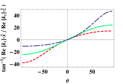
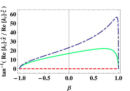
Figure 1: The orientation angle of $\mbox{Re}\,{\bf k}_{t}$ (in degree) plotted against angle of incidence $\theta\in\left(-90^{\circ},90^{\circ}\right)$ for $\beta=-0.5$ (broken curve, red), $\beta=0$ (solid curve, green), and $\beta=0.7$ (broken dashed curve, blue); and plotted against relative speed $\beta\in\left(-1,1\right)$ for $\theta=0^{\circ}$ (broken curve, red), $\theta=45^{\circ}$ (solid curve, green), and $\theta=75^{\circ}$ (broken dashed curve, blue). The refracting half–space is occupied by material A ($\epsilon^{\prime}=6+0.05i$).

For the purposes of illustration, let us suppose firstly that the material occupying the half–space $z>0$ has a relative permittivity $\epsilon^{\prime}=6+0.05i$. We call this material A. We note that the case for the corresponding nondissipative material, specified by a real–valued relative permittivity of 6, was investigated previously using an approach based on the Minkowski constitutive relations [12]. The orientation angle of the real part of ${\bf k}_{t}$, as defined by $\tan^{-1}\left(\kappa/\mbox{Re}\,k_{zt}\right)$, is plotted in Fig. 1 versus (a) angle of incidence $\theta$ for the relative speeds $\beta\in\left\{-0.5,\,0,\,0.7\right\}$; and (b) relative speed $\beta$ for the angles of incidence $\theta\in\left\{0^{\circ},\,45^{\circ},\,75^{\circ}\right\}$. We see that: (a) for a fixed angle of incidence $\theta$, the orientation angle of $\mbox{Re}\,{\bf k}_{t}$ increases as $\beta$ increases (with the exception of the case of normal incidence wherein the orientation angle of $\mbox{Re}\,{\bf k}_{t}$ is $0^{\circ}$ for all values of $\beta$); and (b) for a fixed relative speed $\beta$, the orientation angle of $\mbox{Re}\,{\bf k}_{t}$ increases as $\theta$ increases. Significantly, $\tan^{-1}\left(\kappa/\mbox{Re}\,k_{zt}\right)>0\;(<0)$ for all values of $\beta$, provided that $\theta>0\;(<0)$. Thus, we see that refraction at the interface $z=0$ is always positive, regardless of the values of $\beta$ and $\theta$.

Next we turn to energy flux in the half–space $z>0$, as provided by the cycle–averaged Poynting vector ${\bf P}_{t}$. In the limit $|{\bf r}|\to 0$, we have [6]

$$\left.{\bf P}_{t}\,\right|_{{\bf r}={\bf 0}} = \frac{1}{2}\left[\left(\mbox{Re}\,{\bf e}_{t}\right)\times\left(\mbox{Re}\,{\bf h}_{t}\right)+\left(\mbox{Im}\,{\bf e}_{t}\right)\times\left(\mbox{Im}\,{\bf h}_{t}\right)\right].$$ (16)

The case of incident $s$–polarization state for which

$${\bf e}_{i}=a_{s}\,{\bf e}_{\perp}\equiv a_{s}\,\hat{{\bf y}}$$ (17)

is distinguished from the case of incident $p$–polarization state described by

$${\bf e}_{i}=a_{p}\,{\bf e}_{\parallel}\equiv a_{p}\left(-\cos\theta\,\hat{{\bf x}}+\sin\theta\,\hat{{\bf z}}\right),$$ (18)

with $a_{s,p}$ being complex–valued amplitudes. In Fig. 2, the orientation angle of the cycle–averaged Poynting vector ${\bf P}_{t}$ evaluated in the limit $|{\bf r}|\to 0$, as defined by $\left.\tan^{-1}\left({\bf P}_{t}\mbox{ \tiny{${}^{\bullet}$} }\hat{{\bf x}}/{\bf P}_{t}\mbox{ \tiny{${}^{\bullet}$} }\hat{{\bf z}}\right)\right|_{\,{\bf r}={\bf 0}}$, is plotted versus (a) the angle of incidence $\theta$ for the relative speeds $\beta\in\left\{-0.5,\,0,\,0.7\right\}$, and (b) the relative speed $\beta$ for the angles of incidence $\theta\in\left\{0^{\circ},\,45^{\circ},\,75^{\circ}\right\}$. Also presented in this figure are the corresponding plots of the quantity $\left.{\bf P}_{t}\,\right|_{{\bf r}={\bf 0}}\mbox{ \tiny{${}^{\bullet}$} }\mbox{Re}\,{\bf k}_{t}$ which determines whether the phase velocity is positive or negative. The graphs in Fig. 2 are for the incident plane wave having the $s$–polarization state; the corresponding graphs for the $p$–polarized incident plane wave are almost (but not exactly) identical. The orientation angle of $\left.{\bf P}_{t}\,\right|_{{\bf r}={\bf 0}}$ is observed to (a) increase as $\beta$ increases, at a fixed angle of incidence; and (b) increase as $\theta$ increases, at a fixed relative speed. Furthermore, by comparing Figs. 1 and 2, it is apparent that counterposition of $\left.{\bf P}_{t}\,\right|_{{\bf r}={\bf 0}}$ and $\mbox{Re}\,{\bf k}_{t}$ occurs when $-\beta$ is sufficiently large for $\theta>0$, and when $\beta$ is sufficiently large for $\theta<0$. Counterposition does not occur at all when $\beta=0$, regardless of the angle of incidence. In addition, the phase velocity of the refracted plane wave is positive for all values of $\beta$ and $\theta$.

Let us now consider a second numerical example where the dissipative material occupying $z>0$ possesses the relative permittivity $\epsilon^{\prime}=-0.34+0.04i$. This material, which we call material B, has the relative permittivity of aluminium at the free–space wavelength $\lambda_{\scriptscriptstyle 0}=103$ nm [15]. Material B is radically different from material A insofar as the former can support NPV propagation at rest, as we demonstrate in the following.

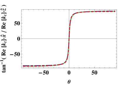
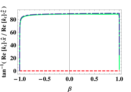
Figure 3: As Fig. 1 except that material A is replaced by material B ($\epsilon^{\prime}=-0.34+0.04i$).

The orientation angle of the real part of ${\bf k}_{t}$ is plotted in Fig. 3 versus (a) the angle of incidence $\theta$ for the relative speeds $\beta\in\left\{-0.5,\,0,\,0.7\right\}$, and (b) the relative speed $\beta$ for the angles of incidence $\theta\in\left\{0^{\circ},\,45^{\circ},\,75^{\circ}\right\}$. We see that: (a) the orientation angle of $\mbox{Re}\,{\bf k}_{t}$ increases uniformly as $\theta$ increases, at approximately the same rate regardless of the value of $\beta$; and (b) for $90^{\circ}>\theta\gtrapprox 10^{\circ}$, the orientation angle of $\mbox{Re}\,{\bf k}_{t}$ is nearly $90^{\circ}$, and for $-90^{\circ}<\theta\lessapprox-10^{\circ}$, the orientation angle of $\mbox{Re}\,{\bf k}_{t}$ is nearly $-90^{\circ}$, regardless of the value of $\beta$. And, in the limits $\beta\to\pm 1$, the orientation angle of $\mbox{Re}\,{\bf k}_{t}$ tends to $0^{\circ}$. Notably, the orientation angle of $\mbox{Re}\,{\bf k}_{t}$ is always $0^{\circ}$ for the case of normal incidence, at all values of $\beta\in\left(-1,1\right)$. As in the previous example, refraction at the interface $z=0$ is positive for all values of $\beta$ and $\theta$.

Graphs of the orientation angle of the cycle–averaged Poynting vector evaluated in the limit $|{\bf r}|\to 0$, analogous to those in Fig. 2, are presented in Fig. 4. Unlike the case for material A, graphs for the incident $s$- and $p$-polarization states are quite different here. The orientation angle of $\left.{\bf P}_{t}\,\right|_{{\bf r}={\bf 0}}$ is observed to be nearly $\pm 90^{\circ}$ for most values of $\beta\in\left(-1,1\right)$ and for $\theta\in\left(-90^{\circ},90^{\circ}\right)$. There exist: (a) a narrow range of values of $\theta$ for a fixed value of $\beta$ (that is centered on $\theta=0^{\circ}$ for $\beta=0$); and (b) a narrow range of values of $\beta$ (that is centered on $\beta=0$ for $\theta=0^{\circ}$) for which the orientation angle of $\left.{\bf P}_{t}\,\right|_{{\bf r}={\bf 0}}$ passes through $0^{\circ}$, as it increases (or decreases) from nearly $-90^{\circ}$ (or $90^{\circ}$) to nearly $90^{\circ}$ (or $-90^{\circ}$). Counterposition of $\left.{\bf P}_{t}\,\right|_{{\bf r}={\bf 0}}$ and $\mbox{Re}\,{\bf k}_{t}$ occurs at $\beta=0$ for the incident $p$-polarization state but not for the incident $s$-polarization state, for all angles of incidence except $\theta=0^{\circ}$ (when $\left.{\bf P}_{t}\,\right|_{{\bf r}={\bf 0}}$ and $\mbox{Re}\,{\bf k}_{t}$ are both directed normally away from the interface). For the incident $s$-polarization state, counterposition occurs when $\beta>0$ for $\theta=0^{\circ}$, $\beta>0.6$ for $\theta=45^{\circ}$, and $\beta>0.92$ for $\theta=75^{\circ}$. For the incident $p$-polarization state, counterposition occurs when $\beta<0$ for $\theta=0^{\circ}$, $\beta<0.6$ for $\theta=45^{\circ}$, and $\beta<0.92$ for $\theta=75^{\circ}$.

The sign of the phase velocity can be inferred from the corresponding plots $\left.{\bf P}_{t}\,\right|_{{\bf r}={\bf 0}}\mbox{ \tiny{${}^{\bullet}$} }\mbox{Re}\,{\bf k}_{t}$ which are also presented in Fig. 4. The phase velocity of the refracted plane wave is positive at $\beta=0$ for all angles of incidence, when the incident plane wave is $s$ polarized. However, when the incident plane wave is $p$ polarized, the refracted plane wave has NPV at $\beta=0$ for $\theta<-3^{\circ}$ and $\theta>3^{\circ}$. For the incident $s$-polarization state, NPV arises in the refracted field when $\beta>0.6$ for $\theta=45^{\circ}$, and $\beta>0.92$ for $\theta=75^{\circ}$. For the incident $p$-polarization state, NPV arises in the refracted field when $\beta<0.6$ for $\theta=45^{\circ}$, and $\beta<0.92$ for $\theta=75^{\circ}$.

3 Beam propagation through a moving slab

3.1 Theoretical considerations

Suppose now that the uniformly moving material which occupied the half–space $z>0$ in §2 is restricted in its extent to a slab region occupying $0<z<L$. As before, the uniformly moving material is described by the constitutive relations (1) in the inertial reference frame $\Sigma^{\prime}$. The regions $z>L$ and $z<0$ are vacuous.

With respect to the inertial reference frame $\Sigma$, a two–dimensional beam with electric field phasor [16]

$${\bf E}_{i}=\int^{\infty}_{-\infty}{\bf e}_{i}(\psi)\,\Psi(\psi)\,\exp\left[i\left({\bf k}_{i}\mbox{ \tiny{${}^{\bullet}$} }{\bf r}-\omega t\right)\right]\;d\psi,\hskip 71.13188ptz\leq 0$$ (19)

is incident upon the uniformly moving slab at a mean angle $\theta$ relative to the slab’s thickness direction $\hat{z}$. The beam is an angular spectrum of plane waves, with each planewave contributor having the wavevector

$${\bf k}_{i}=k_{\scriptscriptstyle 0}\left[\left(\psi\,\cos\theta+\sqrt{1-\psi^{2}}\,\sin\theta\right)\hat{{\bf x}}-\left(\psi\,\sin\theta-\sqrt{1-\psi^{2}}\,\cos\theta\right)\hat{{\bf z}}\,\right].$$ (20)

A Gaussian form

$$\Psi(\psi)=\frac{k_{\scriptscriptstyle 0}\,w_{\scriptscriptstyle 0}}{\sqrt{2\pi}}\,\exp\left[-\frac{\left(k_{\scriptscriptstyle 0}\,w_{\scriptscriptstyle 0}\,\psi\right)^{2}}{2}\right]$$ (21)

is adopted for the angular–spectral function $\Psi(\psi)$, with $w_{\scriptscriptstyle 0}$ being the width of the beam waist [16]. Two polarization states are considered: the $s$-polarization state described by (17) and the $p$-polarization state for which

$${\bf e}_{i}(\psi)=a_{p}\,{\bf e}_{\parallel}\equiv a_{p}\left[\left(\psi\,\sin\theta-\sqrt{1-\psi^{2}}\,\cos\theta\right)\hat{{\bf x}}+\left(\psi\,\cos\theta+\sqrt{1-\psi^{2}}\,\sin\theta\right)\hat{{\bf z}}\right].$$ (22)

As the velocity is tangential to the interfaces and lies wholly in the plane of incidence, the reflected and transmitted beams have spatial Fourier representations similar to that of the incident beam given by (19). In $\Sigma$, the reflected beam is represented by the electric field phasor

$${\bf E}_{r}=\int^{\infty}_{-\infty}{\bf e}_{r}(\psi)\,\Psi(\psi)\,\exp\left[i\left({\bf k}_{r}\mbox{ \tiny{${}^{\bullet}$} }{\bf r}-\omega t\right)\right]\;d\psi,\hskip 71.13188ptz\leq 0,$$ (23)

with the wavevector of each planewave contributor being

$${\bf k}_{r}=k_{\scriptscriptstyle 0}\left[\left(\psi\,\cos\theta+\sqrt{1-\psi^{2}}\,\sin\theta\right)\hat{{\bf x}}+\left(\psi\,\sin\theta-\sqrt{1-\psi^{2}}\,\cos\theta\right)\hat{{\bf z}}\,\right]$$ (24)

and the corresponding amplitudes

$${\bf e}_{r}(\psi)=\left\{\begin{array}[]{ccr}r_{s}\,{\bf e}_{\perp}&\mbox{for}&{\bf e}_{i}(\psi)={\bf e}_{\perp},\vspace{6pt}\\ r_{p}\Big{[}-\left(\psi\,\sin\theta-\sqrt{1-\psi^{2}}\,\cos\theta\right)\hat{{\bf x}}&&\\ +\left(\psi\,\cos\theta+\sqrt{1-\psi^{2}}\,\sin\theta\right)\hat{{\bf z}}\Big{]}&\mbox{for}&{\bf e}_{i}(\psi)={\bf e}_{\parallel}.\end{array}\right.$$ (25)

Likewise, in $\Sigma$, the transmitted beam is represented by the electric field phasor

$${\bf E}_{\tau}=\int^{\infty}_{-\infty}{\bf e}_{\tau}(\psi)\,\Psi(\psi)\,\exp\left\{i\left[{\bf k}_{\tau}\mbox{ \tiny{${}^{\bullet}$} }\left({\bf r}-L\hat{{\bf z}}\right)-\omega t\,\right]\right\}\;d\psi,\hskip 71.13188ptz\geq L,$$ (26)

with ${\bf k}_{\tau}={\bf k}_{i}$ and the amplitudes

$${\bf e}_{\tau}(\psi)=\left\{\begin{array}[]{ccr}\tau_{s}\,{\bf e}_{\perp}&\mbox{for}&{\bf e}_{i}(\psi)={\bf e}_{\perp},\vspace{6pt}\\ \tau_{p}\,{\bf e}_{i}(\psi)&\mbox{for}&{\bf e}_{i}(\psi)={\bf e}_{\parallel}.\end{array}\right.$$ (27)

The electric field phasors for the reflected and transmitted beams in $\Sigma$ are calculated via the strategy outlined in §2. That is, first the problem is transformed to the inertial reference frame $\Sigma^{\prime}$ wherein the boundary-value problem is solved for each planewave contributor to the incident beam, using expressions for the reflection coefficients $r_{s,p}$ and transmission coefficients $\tau_{s,p}$ appropriate for $\Sigma^{\prime}$ [12]. Then the electric phasors for the contributor plane waves are transformed back to $\Sigma$, and integrated with respect to $\psi$ to yield ${\bf E}_{r,\tau}$.

3.2 Numerical studies

The slab thickness was fixed at $L=3\lambda_{\scriptscriptstyle 0}$. Following §2.2, we begin by considering a slab made of material A ($\epsilon^{\prime}=6+0.05i$). In Fig. 5, the reflectance $\left|r_{s}/a_{s}\right|^{2}$ and transmittance $\left|\tau_{s}/a_{s}\right|^{2}$, are plotted against the angle of incidence $\theta\in\left(-90^{\circ},90^{\circ}\right)$, for the relative speeds $\beta\in\left\{-0.5,\,0,\,0.7\right\}$. The reflectance at the angles of incidence $\theta$ and $-\theta$ are the same for $\beta=0$, but this is not true for $\beta\neq 0$; and the same is true for the transmittance. The reflectances and transmittances oscillate markedly as $\theta$ increases. This effect — which is due to multiple reflections at the $z=0$ and $z=L$ interfaces — disappears as the slab thickness increases (as we confirmed in calculations not displayed here). The graphs for the reflectance $\left|r_{p}/a_{p}\right|^{2}$ and transmittance $\left|\tau_{p}/a_{p}\right|^{2}$ (which are not displayed here) are similar to those for $\left|r_{s}/a_{s}\right|^{2}$ and $\left|\tau_{s}/a_{s}\right|^{2}$.

For a mean angle of incidence $\theta=45^{\circ}$, with the incident beam focussed on $\left\{x=0,z=0\right\}$ with waist $w_{\scriptscriptstyle 0}=\lambda_{\scriptscriptstyle 0}$, we investigated the reflected and transmitted beams at the relative speeds $\beta\in\left\{-0.5,\,0,\,0.7\right\}$. The energy density

$$|{\bf E}|^{2}=\left\{\begin{array}[]{lcr}|{\bf E}_{i}+{\bf E}_{r}|^{2}&\mbox{for}&z\leq 0,\vspace{4pt}\\ |{\bf E}_{\tau}|^{2}&\mbox{for}&z\geq L.\end{array}\right.$$ (28)

was used for this purpose.

This energy densities at the planes $z=-L$ and $z=L$ are plotted versus $x\in\left(-10\lambda_{\scriptscriptstyle 0},10\lambda_{\scriptscriptstyle 0}\right)$ in Fig. 6 for both incident polarization states. As $\beta$ decreases, the energy density of the transmitted beam is concentrated at lower values of $x$. Indeed, for both incident $s$- and $p$-polarized beams, the transmitted beam emerges from the moving slab at locations with $x<0$ when $\beta=-0.5$. This is in consonance with the orientation of the corresponding cycle–averaged Poynting vectors, as presented in Fig. 2. We note that the maximum amplitude of the energy density of the transmitted beam decreases as $\beta$ decreases for the incident $s$-polarization state, but this is not the case for the incident $p$-polarization state. Also, the maximum amplitude of the energy density of the reflected beam increases as $\beta$ decreases for the incident $s$-polarization state but decreases as $\beta$ decreases for the other incident polarization state. Extrapolating from Fig. 6, we estimate that at $\beta\approx 0.2$ the energy density of the transmitted beam would be concentrated at $x=3\lambda_{\scriptscriptstyle 0}$ on the face $z=L$ of the slab. The beam would be essentially undeflected by the moving slab at this relative speed and thereby a degree of concealment of the slab may be achieved [12].

Now, in view of §2.2, we turn to the case where the slab is made of material B ($\epsilon^{\prime}=-0.34+0.04i$). All other parameters are the same as those used for Figs. 5 and 6. The reflectances and transmittances are plotted against the angle of incidence $\theta\in\left(-90^{\circ},90^{\circ}\right)$, for $\beta\in\left\{-0.5,\,0,\,0.7\right\}$ in Fig. 7. The graphs of the reflectances and transmittances are symmetric about $\theta=0^{\circ}$ for $\beta=0$, but they are asymmetric for $\beta\neq 0$. We note that the magnitudes of the transmittances are very much smaller than those of the reflectances, with the largest transmittances occurring when the relative speed $\beta$ is largest. The oscillations apparent in Fig. 5 are largely absent from the graphs of the reflectances and transmittances in Fig. 7. This is because of the much greater degree of attenuation within the uniformly moving slab in the present case.

The beam energy densities at $z=-L$ and $z=L$ are mapped across $x\in\left(-10\lambda_{\scriptscriptstyle 0},\,10\lambda_{\scriptscriptstyle 0}\right)$ in Fig. 8 for $\beta\in\left\{-0.5,\,0,\,0.7\right\}$, at a mean angle of incidence $\theta=45^{\circ}$. Only the plots for the incident $s$–polarized beam are presented here; the corresponding plots for the incident $p$–polarized beam are similar. For both incident polarization states, the energy density of the transmitted beam — which is very much lower than that of the reflected beam — decreases greatly as the relative speed $\beta$ decreases. This is in keeping with the behaviours of the corresponding reflectances and transmittances, as presented in Fig. 7. Furthermore, the energy density of the transmitted beam is largely directed normally, away from the interface $z=L$. This may be explained by considering the direction of the corresponding cycle–averaged Poynting vector, as presented in Fig. 4. The cycle–averaged Poynting vector is approximately aligned with $\hat{{\bf z}}$ for an angle of incidence of approximately $55^{\circ}$ for $\beta=0.7$. Thus, the maximums of the transmittances at $\theta\approx 55^{\circ}$ for $\beta=0.7$ give rise to the maximums in the transmitted energy density in the direction of $\hat{{\bf z}}$ for $\beta=0.7$ observed in Fig. 8. And similarly for the instances where $\beta=0$ and $\beta=-0.5$, but here the energy densities of the transmitted beams are much lower.

4 Concluding remarks

By directly implementing the Lorentz transformations of the electric and magnetic fields, we have confirmed that counterposition and NPV are not Lorentz-covariant phenomenons, in the context of dissipative mediums. This finding had previously been established for nondissipative mediums using the Minkowski constitutive relations [9, 12]. We further demonstrated that the lateral position of a Gaussian beam, upon traversal through a uniformly moving slab, as perceived by a nonco–moving observer, could be controlled by varying the slab’s velocity, when the velocity is tangential to the interfaces and lies wholly in the plane of incidence. Two instances are especially noteworthy: (i) at certain velocities, the transmitted beam can emerge from the slab laterally displaced in the direction opposite to the direction of incident beam; and (ii) at a unique slab velocity, the beam can emerge from the slab with no lateral shift in its position, thereby achieving a degree of concealment for the slab [12]. For a uniformly moving slab made of a material which supports both positive and negative phase velocity when at rest (material B in the previous sections), it was seen that the transmittances are very small and the energy density of the transmitted beam is largely concentrated in the direction normal to the slab, regardless of the inertial frame of reference.

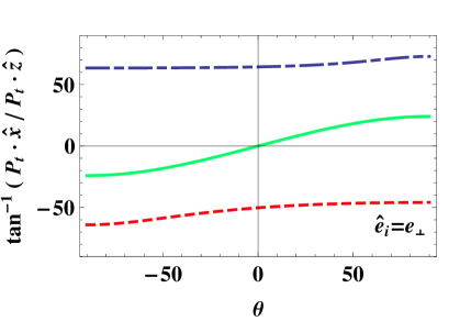
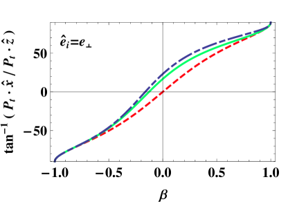
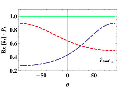
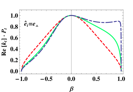
Figure 2: The orientation angle of the cycle–averaged Poynting vector ${\bf P}_{\,t}$ and the quantity ${\bf P}_{t}\mbox{ \tiny{${}^{\bullet}$} }\mbox{Re}\,{\bf k}_{t}$ (normalized) plotted against angle of incidence $\theta\in\left(-90^{\circ},90^{\circ}\right)$ for $\beta=-0.5$ (broken curve, red), $\beta=0$ (solid curve, green), and $\beta=0.7$ (broken dashed curve, blue); and plotted against relative speed $\beta\in\left(-1,1\right)$ for $\theta=0^{\circ}$ (broken curve, red), $\theta=45^{\circ}$ (solid curve, green), and $\theta=75^{\circ}$ (broken dashed curve, blue). The refracting half–space is occupied by material A ($\epsilon^{\prime}=6+0.05i$). Plots are shown for the incident $s$-polarization state.

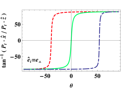
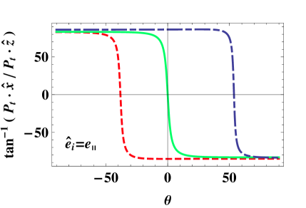
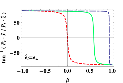
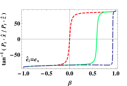
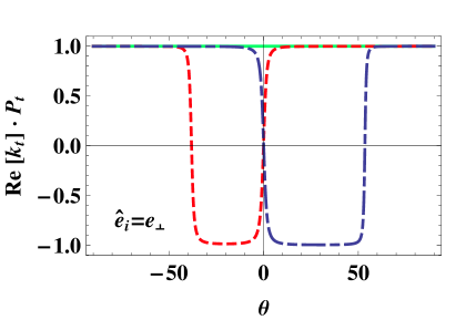
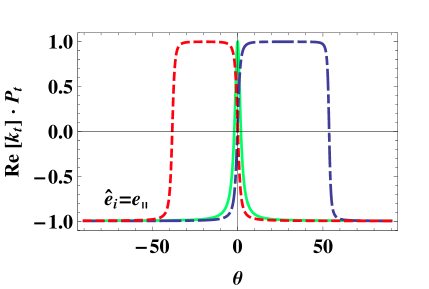
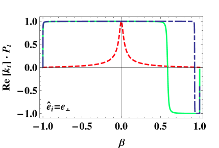
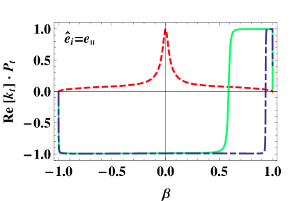
Figure 4: As Fig. 2 except that material A is replaced by material B ($\epsilon^{\prime}=-0.34+0.04i$), and here the plots for the incident $s$-polarization state (left) are quite different to the corresponding plots for the incident $p$-polarization state (right).

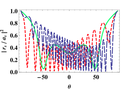
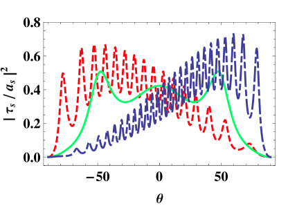
Figure 5: The reflectance $\left|r_{s}/a_{s}\right|^{2}$ and transmittance $\left|\tau_{s}/a_{s}\right|^{2}$, plotted against angle of incidence $\theta\in\left(-90^{\circ},90^{\circ}\right)$, for $\beta=-0.5$ (broken curve, red), $\beta=0$ (solid curve, green), and $\beta=0.7$ (broken dashed curve, blue). The moving slab of thickness $L=3\lambda_{\scriptscriptstyle 0}$ is made of material A ($\epsilon^{\prime}=6+0.05i$).

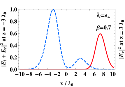
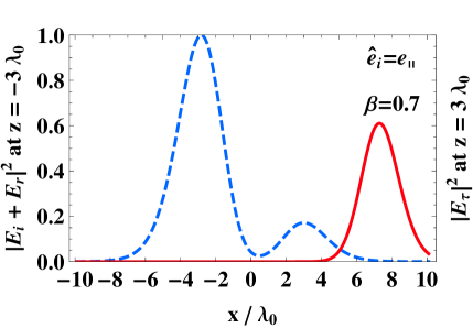
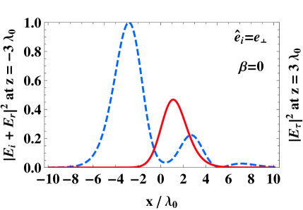
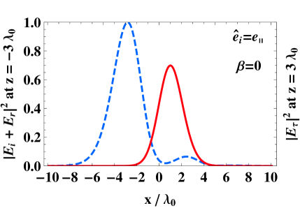
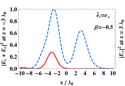
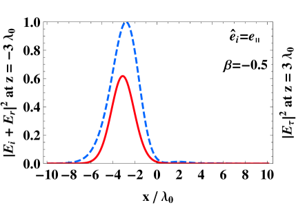
Figure 6: The energy densities at $z=3\lambda_{\scriptscriptstyle 0}$ (solid curves, red) and $z=-3\lambda_{\scriptscriptstyle 0}$ (broken curves, blue) plotted against $x\in\left(-10\lambda_{\scriptscriptstyle 0},10\lambda_{\scriptscriptstyle 0}\right)$ for $\beta=0.7$ (top), $\beta=0$ (middle), and $\beta=-0.5$ (bottom), for an incident $s$-polarized beam (left) and an incident $p$-polarized beam (right). The moving slab of thickness $L=3\lambda_{\scriptscriptstyle 0}$ is made of material A ($\epsilon^{\prime}=6+0.05i$). The centre of the incident beam impinges on the moving slab at the point $x=0$, $z=0$, at an angle of incidence $\theta=45^{\circ}$.

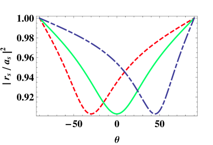
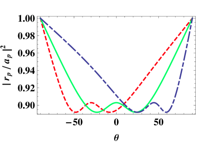
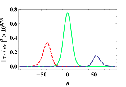
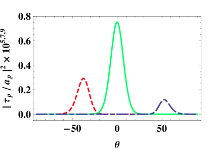
Figure 7: The reflectances $\left|r_{u}/a_{u}\right|^{2}$ and transmittances $\left|\tau_{u}/a_{u}\right|^{2}$, $(u=s,p)$, plotted against angle of incidence $\theta\in\left(-90^{\circ},90^{\circ}\right)$, for $\beta=-0.5$ (broken curve, red), $\beta=0$ (solid curve, green), and $\beta=0.7$ (broken dashed curve, blue). The moving slab of thickness $L=3\lambda_{\scriptscriptstyle 0}$ is made of material B ($\epsilon^{\prime}=-0.34+0.04i$). The transmittances are multiplied by $10^{7}$ for $\beta=-0.5$, by $10^{9}$ for $\beta=0$, and $10^{5}$ for $\beta=0.7$.

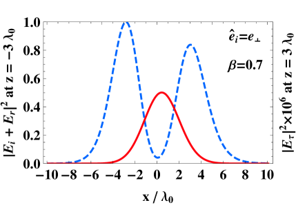
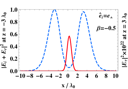
Figure 8: As Fig. 6 except that material A is replaced by material B ($\epsilon^{\prime}=-0.34+0.04i$). Only the graphs for the incident $s$–polarized beam are presented.

References

- [1] Ramakrishna S A 2005 Physics of negative refractive index materials Rep. Prog. Phys. 68 449–521
- [2] Lakhtakia A, McCall M W and Weiglhofer W S 2002 Brief overview of recent developments on negative phase-velocity mediums (alias left-handed materials) Arch. Elektron. Übertr. 56 407–410
- [3] McCall M W, Lakhtakia A and Weiglhofer W S 2002 The negative index of refraction demystified Eur. J. Phys. 23 353–359
- [4] Belov P A 2003 Backward waves and negative refraction in uniaxial dielectrics with negative dielectric permittivity along the anisotropy axis Microwave Opt. Technol. Lett. 37 259–263
- [5] Mackay T G and Lakhtakia A 2009 (submitted for publication)
- [6] Chen H C 1983 Theory of Electromagnetic Waves (New York: McGraw–Hill)
- [7] Zhang Y, Fluegel B and Mascarenhas A 2003 Total negative refraction in real crystals for ballistic electrons and light Phys. Rev. Lett. 91 157404
- [8] Lakhtakia A and McCall M W 2004 Counterposed phase velocity and energy–transport velocity vectors in a dielectric–magnetic uniaxial medium Optik 115 28–30
- [9] Grzegorczyk T M and Kong J A 2006 Electrodynamics of moving media inducing positive and negative refraction Phys. Rev. B 74 033102
- [10] Mackay T G and Lakhtakia A 2007 Counterposition and negative refraction due to uniform motion Microwave Opt. Technol. Lett. 49 874–876
- [11] We note that the phenomenon of counterposition is referred to as ‘negative refraction’ in Ref. [9]. In contrast, and in keeping with Snel’s law [6], we adopt the standard convention wherein the sense of refraction is determined solely by the relative orientations of the real parts of the refraction and incidence wavevectors.
- [12] Mackay T G and Lakhtakia A 2007 Concealment by uniform motion J. Euro. Opt. Soc. – Rapid Pub. 2 07003
- [13] Besieris I M and Compton Jr R T 1967 Time–dependent Green’s function for electromagnetic waves in moving conducting media J. Math. Phys. 8 2445–2451
- [14] Mackay T G and Lakhtakia A 2009 Positive–, negative–, and orthogonal–phase–velocity propagation of electromagnetic plane waves in a simply moving medium: reformulation and reappraisal Optik 120 45–48
- [15] Ditchburn R W and Freeman G H C 1966 The optical constants of aluminium from 12 to 36 eV Proc. R. Soc. Lond. A 294 20–37
- [16] Haus H A 1984 Waves and Fields in Optoelectronics (Englewood Cliffs, NJ: Prentice–Hall)