ELLIPTIC FLOW: A STUDY OF SPACE-MOMENTUM CORRELATIONS IN RELATIVISTIC NUCLEAR COLLISIONS
Abstract
Here I review measurements of , the second component in a Fourier decomposition of the azimuthal dependence of particle production relative to the reaction plane in heavy-ion collisions. is an observable central to the interpretation of the subsequent expansion of heavy-ion collisions. Its large value indicates significant space-momentum correlations, consistent with the rapid expansion of a strongly interacting Quark Gluon Plasma. Data is reviewed for collision energies from to 200 GeV. Scaling observations and comparisons to hydrodynamic models are discussed.
1 Introduction
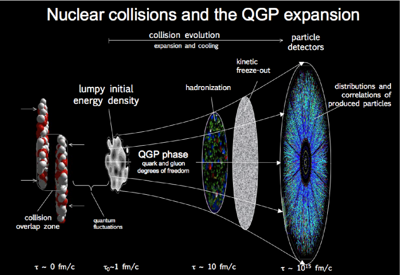
Collisions of heavy nuclei have been exploited for decades to search for and study the transition of hadronic matter to quark gluon plasma[1, 2]. In these collisions, the extended overlap area, where the nuclei intersect and initial interactions occur, does not possess sphrerical symmetry in the transverse plane. Rather, for non-central collisions, the overlap area is roughly elliptic in shape. If individual nucleon-nucleon collisions within the interaction region are independent of each other (e.g. point-like) and no subsequent interactions occur, this spatial anisotropy will not be reflected in the momentum distribution of particles emitted from the interaction region. On the other hand, if the initial interactions are not independent, or if there are subsequent interactions after the initial collisions, then the spatial anisotropy can be converted into an anisotropy in momentum-space. The extent to which this conversion takes place allows one to study how the system created in the collision of heavy nuclei deviates from a point-like, non-interacting system. The existence and nature of space-momentum correlations is therefore an interesting subject in the study of heavy ion collisions and the nature of the matter created in those collisions[3, 4]. Fig. 1 shows an illustration of the possible stages of a heavy-ion collisions starting with some initial energy density deposited at mid-rapidity, followed by a QGP expansion, a hadronization phase boundary, a kinetic freeze-out boundary and finally the observation of particle trajectories in a detector.
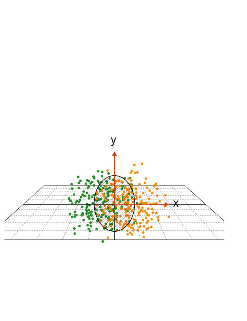
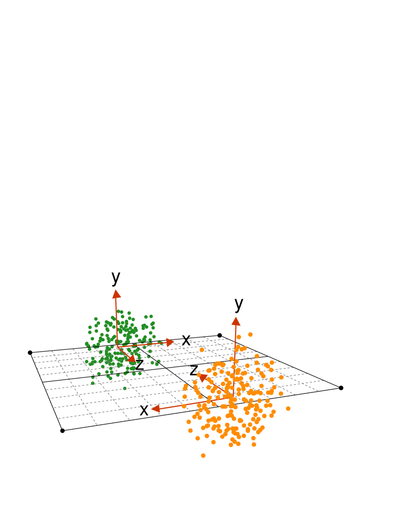
One can consider a number of ways to study space-momentum correlations: e.g. two-particle correlations[5] and HBT[6, 7]. In this review we discuss elliptic flow ; an observable that has been central in the interpretation of heavy-ion data and QGP formation[8]. Given the predominantly elliptic shape of the initial overlap region, it is natural to ask whether this shape also shows up in the distribution of particles in momentum-space. Fig. 2 shows a schematic illustration of the conversion of coordinate-space anisotropy to anisotropy in momentum-space. The left panel shows the position of nucleons in two colliding nuclei at the moment of impact. The overlap region is outlined and shaded. A Fourier decomposition can be used to describe the azimuthal dependence of the final triple momentum-space distributions[9]:
| (1) |
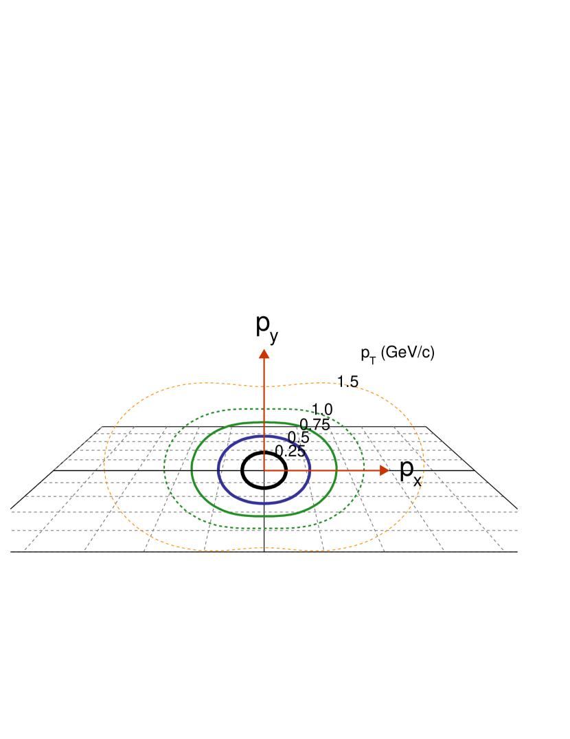
where is the azimuth angle of the particle, the longitudinal rapidity variable, the transverse momentum, and is the reaction plane angle defined by the vector connecting the centers of the two colliding nuclei. Positive implies that more particles are emitted along the short axis of the overlap region. To study the extent to which space-momentum correlations develop in heavy-ion collisions, one can measure the second component and compare it to the initial spatial eccentricity[3, 10]. The right panel of Fig. 2 shows the final azimuthal distribution of particles in momentum-space. The curves represent the anisotropy at different values measured in 200 GeV Au+Au collisions[11]: i.e. . The goal of measurements is to study how the initial spatial anisotropy in the left panel is converted to the momentum-space anisotropy in the right panel. In this review, a summary of data for different colliding systems, different center-of-mass energies, and different centralities is given.
This review will focus on results from the first four years of operation of the Relativistic Heavy Ion Collider (RHIC). We start with a brief discussion of the beam energy dependence of and some ideas about what physics might be relevant. Even before considering physics scenarios to explain how a space-momentum correlation develops, one can see that to interpret it is important to understand the initial geometry and how it varies with the collision centrality and system-size. Since, the concept of the reaction-plane is so central to the definition of and eccentricity is so central to it’s interpretation, I discuss the two in a sub-section below. Then a review of RHIC data is provided. This will include the dependence of on center-of-mass energy, centrality, colliding system, pseudo-rapidity, , particle mass, constituent quark number and various scaling laws. In the following section, I will discuss comparisons to models and the emergence of the hydrodynamic paradigm at RHIC. Particular emphasis is given to uncertainties in the model comparisons. In that section I will also discuss current attempts to extract viscosity and future directions of investigation.
Voloshin, Poskanzer, and Snellings recently wrote a review article[12] on collective phenomena in non-central nuclear collisions that deals with a similar subject matter. That article provides valuable detail on technical aspects of measuring . In this review I will attempt to avoid duplicating that work by discussing interpretations of more extensively and refer the reader to that review where appropriate.
1.1 Two Decades in Time and Five Decades in Beam Energy
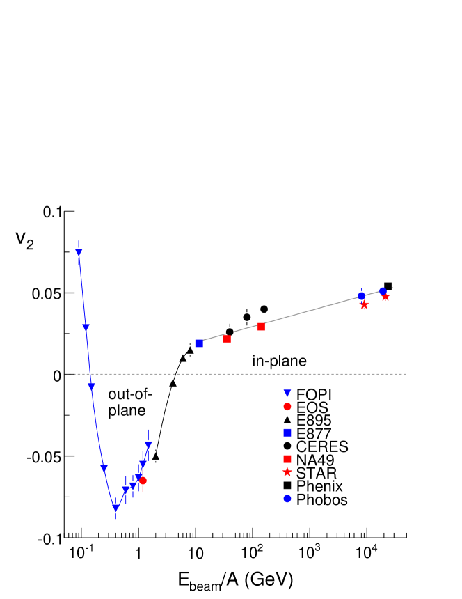
Positive values of imply that particles tend to be produced more abundantly in the direction than in the direction. This is referred to as in-plane flow. Fig. 3 shows measured in an interval of beam energies covering five orders of magnitude[13, 14, 15, 16, 17, 18, 19, 20, 21, 22]. For ranging from approximately GeV ( GeV), is negative. For this energy range, spectator protons and neutrons are still passing the interaction region while particles are being produced. Their presence inhibits particle emission in the in-plane direction leading to the phenomenon termed squeeze-out. At still lower energies, is positive as the rotation of the matter leads to fragments being emmitted in-plane. At this energy beam rapidity and mid-rapidity are essentially indistinguishable with units.
In-plane flow: As the beam energy is increased, the nuclei become more Lorentz contracted and the time it takes the spectators to pass each other decreases. It was predicted by Ollitrault[3] that at high enough beam energy, the squeeze-out phenomena would cease and would take on positive values. Positive values were measured at the AGS for energies above GeV ( GeV). For energies above GeV ( GeV), exhibits a steady log-linear increase: or where the data represented are from intermediate impact parameter A+A collsions. It appears therefore that RHIC data may be part of a smooth trend that began at SPS energies. This trend was noted previously at least once[23]. Understanding the physics that underlies that trend is one of the challenges of heavy-ion physics.
One class of models that has provided an illustrative reference for heavy-ion collisions are hydrodynamic models which are used to model the expansion the matter remaining in the fireball after the initial collisions[24, 25, 26, 27, 28, 29, 30, 31, 32, 33]. This model can be used to determine how matter with a vanishingly small mean free path would convert the initial eccentricity into . These models typically treat all elliptic flow as arising from the final state expansion rather than from some initial state effects[34, 35, 36, 37]. In the hydrodynamic models, large pressure gradients in the in-plane direction lead to a preferential flow of matter in the in-plane direction. In this review, we will use hydrodynamic models as a convenient reference. Other models providing a valuable reference for measurements include hadronic and partonic cascades and transport models[38, 41, 42, 43, 44, 39, 40, 45, 46]. Additionally, the blast-wave model provides a successful parametrization of low heavy-ion data, including , HBT, and spectra in terms of several freeze-out parameters[30, 47].
1.2 Initial Geometry: The Reaction Plane and Eccentricity
In the collision of two symmetric nuclei, a unique vector (the -axis) can be defined by applying the right-hand-rule to the momentum vector of one nucleus and the vector pointing to the center of the other nucleus. The -axis is a pseudovector. The reaction-plane is then the plane perpendicular to the -axis containing the points at the center of the two nuclei. The reaction-plane and the right-handed coordinate system are illustrated in Fig. 4. The figure contains perspective illustrations of two nuclei approaching with an impact parameter of 6 fm. The impact parameter is the distance between the centers of the two nuclei at the moment of their closest approach. The two nuclei in this illustration are Lorentz contracted by a Lorentz gamma factor of 10 which roughly corresponds to the appropriate gamma for top SPS energies.
The reaction-plane is not directly observed in experiments, however, and this introduces a systematic uncertainty into the measurement of . One often relies instead on indirect observations to estimate [48, 49, 50, 51, 52]. For example, when forming two particle azimuthal correlations such as , a non-zero value will lead to a modulation in of the form . Fig. 5 shows the correlation function for hadrons produced at mid-rapidity at RHIC[53, 54]. The panels show different centralities. The area normalized correlation function is
| (2) |
where and are, respectively, the uncorrected yields of pairs in the same and in mixed events within each data sample. shows a clear dependence. We note here that what is measured in these correlation functions is in anticipation of a discussion of fluctuations.
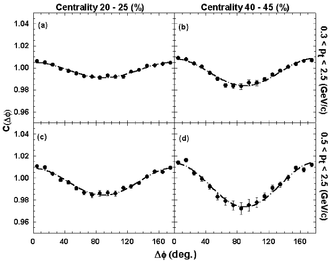
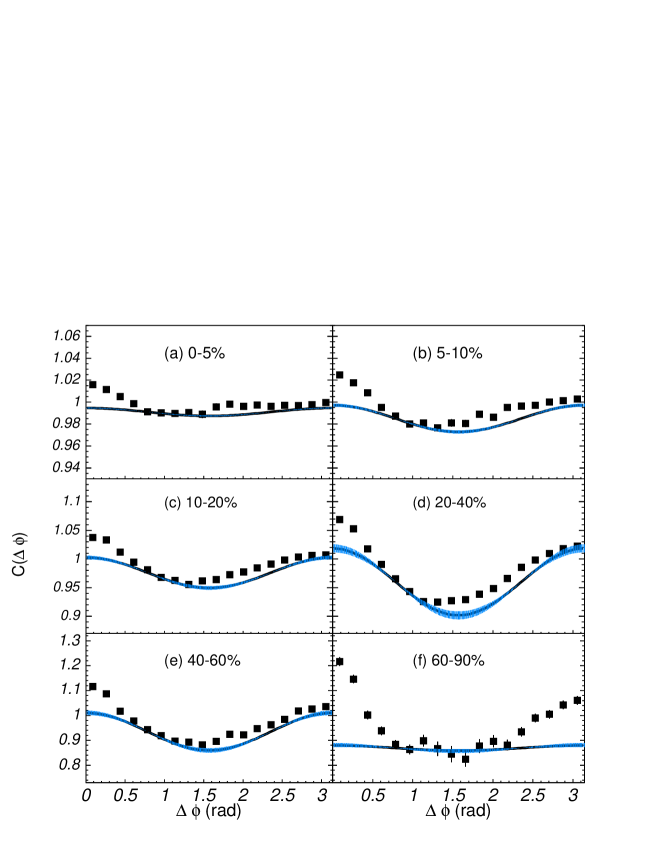
will not be the only contribution to the azimuthal dependence of the two-particle azimuthal correlations. Other processes that are not related to the reaction-plane can give rise to structures in the shape of the two-particle distribution as well. These non-reaction plane contributions are commonly called ”non-flow”. The subject of non-flow is an important one and will be discussed throughout this review. The contribution of non-flow can be seen more clearly by looking at very peripheral collisions or by selecting high momentum particles to increase the chance that a particular pair of hadrons are correlated to a hard scattered parton (jet). Fig. 6 shows the correlation function for higher momentum particles[55]. The solid line shows what a pure correlation would look like[56]. The difference between those curves and the data are often taken as a measurement of jet correlations[55, 57, 58].
Even if the reaction-plane were known with precision, there is no first principles calculation of the initial matter distribution in the overlap region, so the eccentricity is uncertain. Various models can be used to calculate the initial spatial eccentricity which can then be compared to . Defining the axis according to the right-hand-rule, the eccentricity is traditionally calculated as:
| (3) |
where the average represents a weighted mean. Other eccentricity definitions have also been considered[59]. The weights can be some physical quantity in a model such as energy or entropy density, or simply the position of nucleons participating in the collision. One popular method for calculating the eccentricity is to use a Monte Carlo Glauber model. Details can be found in a recent Review[60]. In that model, a finite number of nucleons are distributed in a nucleus according to a Woods-Saxon distribution. Then two nuclei are overlaid with a fixed impact parameter and the and positions of the participating nucleons is determined based on whether the nucleons overlap in the transverse plane; each nucleon is considered to be a disk with an area determined by the dependent nucleon-nucleon cross-section. The and coordinates of the participating nucleons are then used to calculate the eccentricity. Those nucleons that do not participate in this initial interaction are called spectators. One can anticipate that due to the finite number of nucleons in this model, the initial geometry will fluctuate. Other models used to determine the initial matter distribution including HIJING[61], NEXUS[62], and Color Glass Condensate models[63, 64, 65, 66] also reach the same conclusions; the initial overlap region is expected to be lumpy rather than smooth. Fig. 7 shows the gluon density in the transverse plane which is probed by a 0.2 fm quark-antiquark dipole at two different values in the IPsat CGC model[63] ( is in the left panel and in the right panel). The lumpiness is immediately apparent.
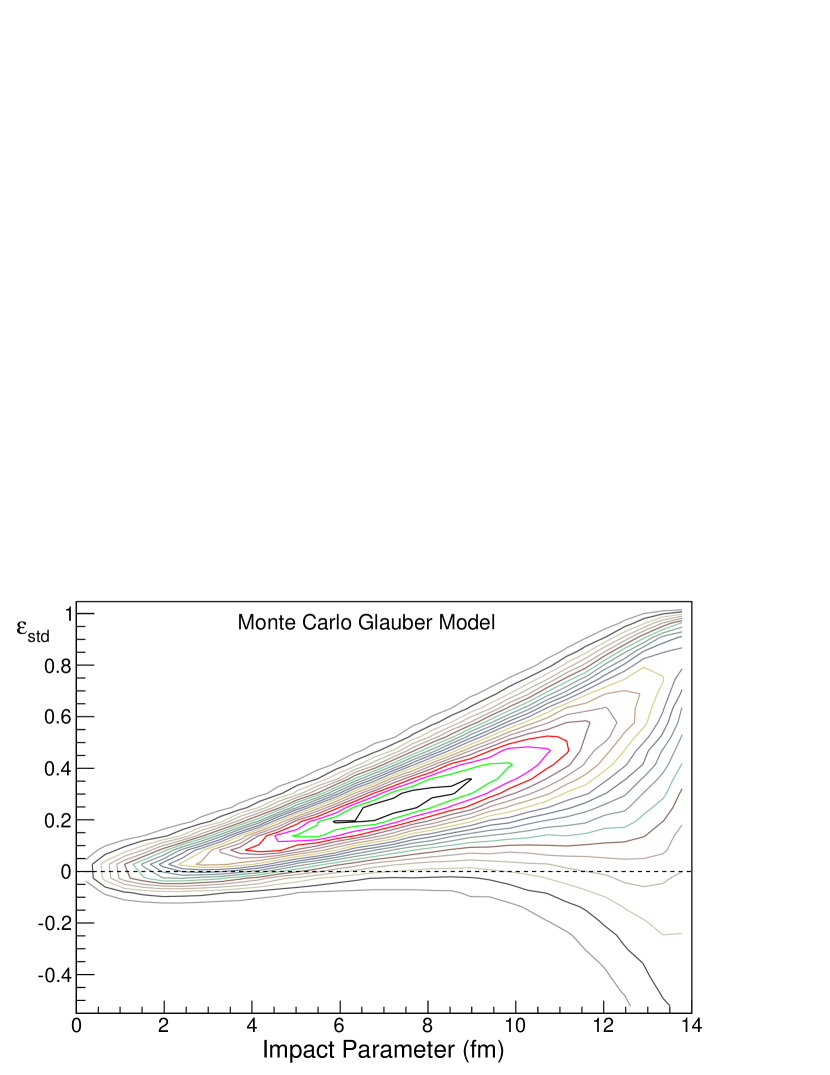
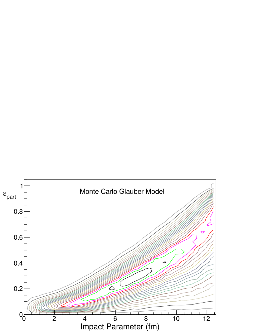
Until recently however[67, 68], data was compared almost exclusively to calculations assuming an infinitely smooth initial matter distribution (for example in initializing a hydrodynamic expansion). Improving on that approximation may be important for understanding the shape expected for the distribution[5, 69]. This distribution is also investigated in heavy ion collisions in order to search for jets. In any scenario where space-momentum correlations develop, the correlations and fluctuations in the initial geometry can be manifested in the distribution and understanding these correlations is important for interpreting heavy-ion collisions. Fluctuations in the initial geometry have also led to the idea of measuring particle distributions relative to the participant-plane rather than the reaction-plane[70, 59]. The participant-plane is defined by the major axis of the eccentricity which, due to fluctuations, can deviate from the reaction-plane. The eccentricity relative to the participant-plane is a positive definite quantity and is always larger than the eccentricity relative to the reaction-plane; the participant-plane is defined by rotating to the axis that maximizes the eccentricity. Fig. 8 shows the event-by-event distribution of the standard eccentricity (left panel) and the participant eccentricity (right panel) as a function of impact parameter determined from a Monte-Carlo Glauber calculation. The fluctuations in this model are large as illustrated by the widths of the distributions. The relationship between the different definitions of eccentricity and their fluctuations are explained clearly in two recent papers[59, 71].
Different models for the initial matter distribution yield different estimates of and . The deviations in the for different models can be of the order of 30% and strongly centrality dependent[72]. That uncertainty in leads to an inherent uncertainty when comparing models to . This level of uncertainty becomes important when attempting to estimate transport properties of the matter based on comparisons of the observed to the initial .
2 Review of Recent Data
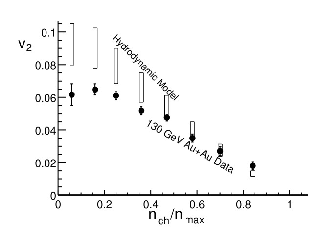
The first paper published on RHIC data was on elliptic flow in GeV Au+Au collisions[18]. Fig. 9 shows that data on the centrality dependence of . The values of reach a maximum of approximately 6% for peripheral collisions where the initial eccentricity of the system is largest. That value is 50% larger than the values reached at SPS energies[21] and the values are a factor of two larger than the those predicted by the RQMD transport-cascade model[42]. For central collisions, the measurements approach the zero mean-free-path limit estimated from the eccentricity shown in the figure as open boxes. The boxes represent the eccentricity scaled by 0.19 (bottom edge of the boxes) and 0.25 (top edge of the boxes). Those values are chosen to represent the typical conversion of eccentricity to in hydrodynamic models. At lower energies, the RQMD model provided a better description of the data, while hydrodynamic models significantly over-predicted the data. The conclusion based on this early comparison, therefore, was that heavy-ion collisions approximately satisfy the assumptions made in the hydrodynamic models: 1) zero mean-free-path between interactions, and 2) early local thermal equilibrium[33]. These conclusions remain at the center of scientific debate in the heavy-ion community.
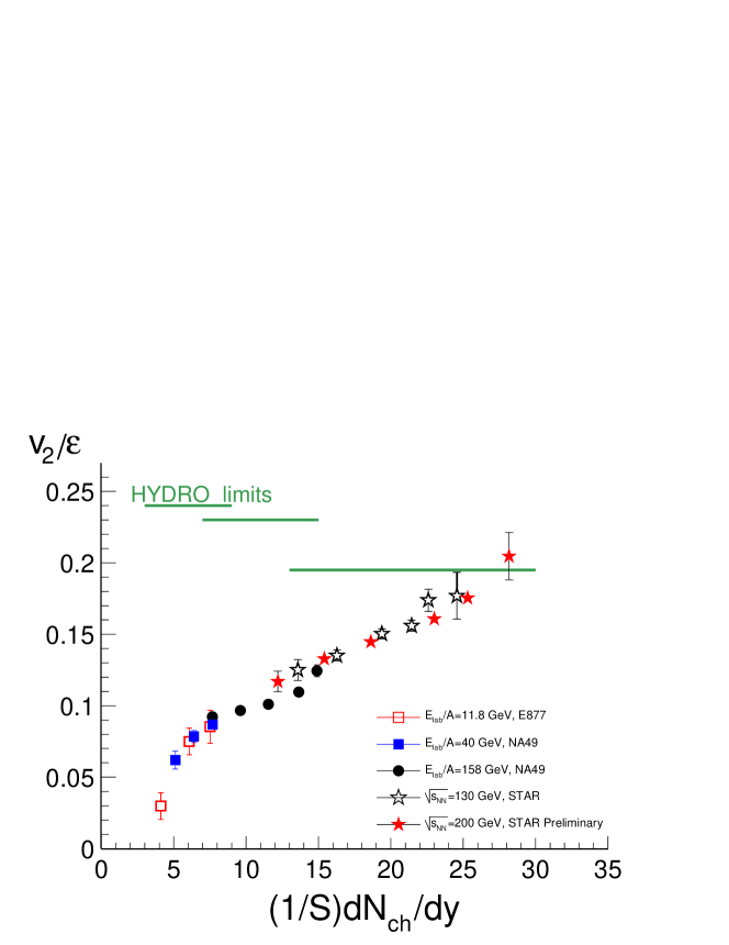
In Fig. 10, is scaled by model calculations of the initial eccentricity and plotted versus transverse particle density [21]. This facilitates comparisons of across different energies, collision centralities and system-sizes[41, 10].
For the case of ballistic expansion of the system – that is an expansion for which the produced particles escape the initial overlap zone without interactions – should only reflect the space-momentum correlations that arise from the initial conditions. Those can exist in the case that the initial interactions are not point-like[34] but rather involve cross-talk between different interactions within the overlap zone. The opposite extreme from the ballistic expansion limit is the zero mean-free-path limit represented by ideal hydrodynamic models. Lacking a length scale, the zero mean-free-path models should not depend on system-size and instead should be a function of density.
The measurements of are expected to rise from values near the ballistic expansion limit and asymptotically approach the zero mean-free-path limit as the density of the system is increased. Data in Fig. 10 exhibit such a behavior with the most central collisions at full RHIC energy apparently becoming consistent with the hydrodynamic model. This conclusion however depends on the model calculations for the initial eccentricity and on the assumption that the observed dominantly arises from an expansion phase where anisotropic pressure gradients are the origin of the space-momentum correlations. Different models for the eccentricity yield results that deviate both in their centrality dependence and in their overall magnitude. Reasonable models for the eccentricity can easily give magnitudes larger than those used in Fig. 10 with a stronger centrality dependence. The ratio can therefore be smaller than what is shown and have a different shape[72]. Given this level of uncertainty, the conclusion that heavy-ion collisions at GeV approximately satisfy the assumptions made in the hydrodynamic models i.e. early local thermal equilibrium and interactions near the zero mean-free path limit, would be more convincing if an asymptotic approach to a limiting value were observed. Rather, for the eccentricity calculation used in Fig. 10, the data suggest a nearly linear rise with no indication of asymptotic behavior.
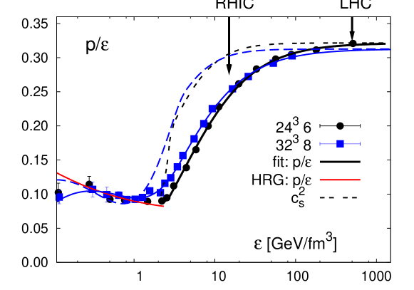
In the hydrodynamic picture, one might also expect that versus will be sensitive to the equation-of-state of the matter formed during the expansion phase. Since is expected to reflect space-momentum correlation developed due to pressure gradients and is a measure of the transverse particle density, versus could be considered as a proxy for the pressure versus energy density or the equation-of-state. It’s difficult to identify in the data the features that are expected in the equation-of-state. Fig. 11 shows the equation-of-state calculated in a recent lattice QCD calculation[73]. The onset of the QGP phase is seen to lead to an increase in the pressure as the energy density is increased above a critical value. The energy density in heavy-ion collisions is often estimated from the Bjorken formula[74]:
| (4) |
which depends only on the experimentally accessible quantity , the overlap area of the nuclei and , the unknown formation time which is often assumed to be 1 fm. The Bjorken estimate for the energy density is closely related to the transverse particle density .
2.1 Differential Elliptic Flow
In addition to studying how integrated over all particles depends on the centrality or of the collision, one can study how depends on the kinematics of the produced particles (differential elliptic flow). Fig. 12 shows the centrality and pseudo-rapidity dependence of for 200 GeV Au+Au collisions[75]. is largest at mid-rapidity where the transverse particle density is largest and then falls off at larger values. This behavior is therefore consistent with the trends seen in integrated where appears to increase with increasing transverse particle density.
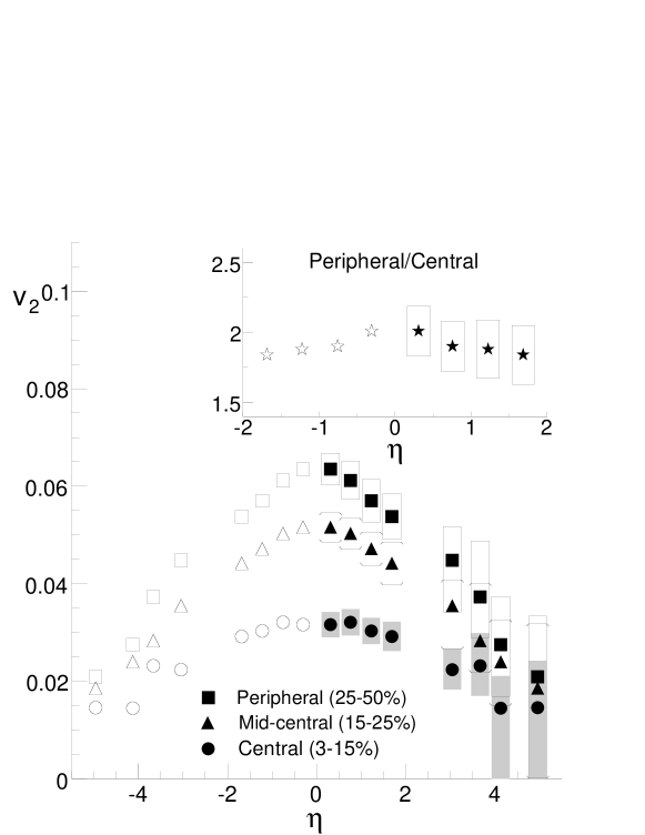
The fall off of with increasing is common to the three centrality intervals studied. The inset of the figure shows the ratio of in peripheral over central collisions. Within errors the ratio is flat indicating a similar shape for all centralities with only changing by a scale factor. Scaling of for different energies and system sizes will be discussed in a later section.
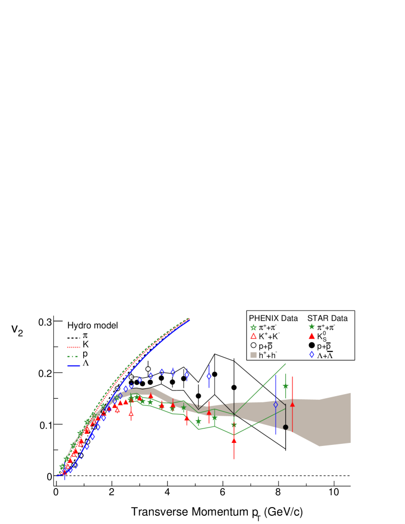
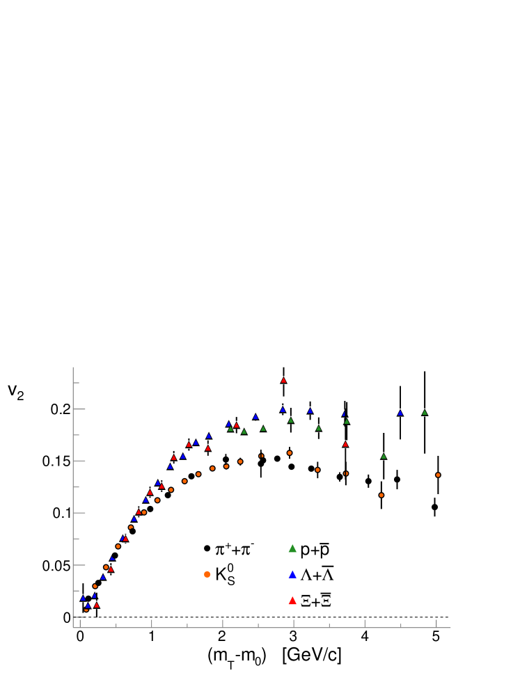
Fig. 13 shows for a variety of particle species as a function of their transverse momentum [76, 77, 78, 79, 80, 81]. In the region below GeV/c, follows mass ordering with heavier particles having smaller at a given . Above this range, the mass ordering is broken and the heavier baryons take on larger values.
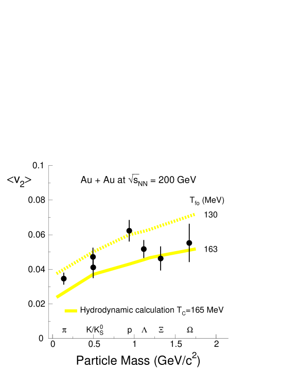
A hydrodynamic model for is also shown which describes the in the lower region well. This mass ordering is a feature expected for particle emission from a boosted source. In the case that particles move with a collective velocity, more massive particles will receive a larger kick. As the particles are shifted to higher , the lower momentum regions become depopulated with a larger reduction in the direction with the largest boost (in-plane). This reduction reduces at a given , with the reduction largest for more massive particles. Note that this does not imply that the more massive particles have a smaller integrated value, and in fact the opposite is true. Fig. 14 shows for identified particles integrated over all [82, 83]. The integration shows that increases with particle mass. This is because the more massive particles have a larger and is generally increasing with in the region where the bulk of the particles are produced. The hydrodynamic model also exhibits this trend.
2.1.1 Identified Particle : RHIC versus SPS
Fig. 15 shows pion and proton from Au+Au[81] and 17.3 GeV Pb+Pb collisions[21]. The centrality intervals have been chosen similarly for the 17.3 GeV and 62.4 GeV data. The STAR data at 62.4 GeV are measured within the pseudo-rapidity interval and the 17.3 GeV data are from the rapidity interval . These intervals represent similar intervals. It has been shown that data for pions and kaons at 62.4 GeV are similar to 200 GeV data; the 62.4 GeV data only tending to be about 5% smaller than the 200 GeV data.
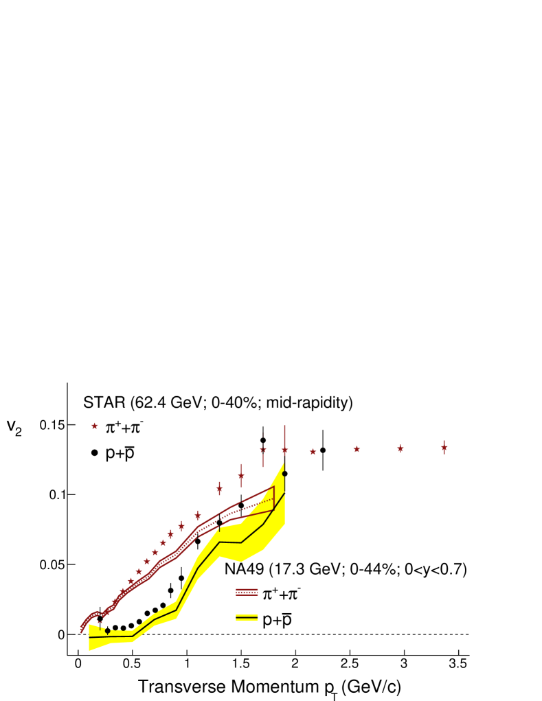
Appreciable differences are seen between the 17.3 GeV and 62.4 GeV data. At GeV/c, for both pions and protons, the values measured at 62.4 GeV are approximately 10%–25% larger than those measured at 17.3 GeV. Although the magnitude of is different at the lower energy, the systematics of the particle-type dependencies are similar. In particular, pion and proton cross over each other at near GeV/c for 17.3, 62.4 and 200 GeV data. Due to the limited kinematic range covered by the 17.3 GeV data, it’s not possible to determine if the of baryons at GeV becomes larger than that for the lighter mesons.
The increase in the magnitude of from 17.3 GeV to 62.4 GeV and the similarity of 62.4 GeV to 200 GeV has been taken as a possible indication for the onset of a limiting behavior[84]. In a collisional picture, a saturation of could indicate that for at and above 62.4 GeV the number of collisions the system constituents experience in a given time scale can be considered large and that hydrodynamic equations can therefore be applied. Hydrodynamic model calculations of depend on the model initialization and the poorly understood freeze-out assumptions. As such, rather than comparing the predicted and measured values at one energy, the most convincing way to demonstrate that a hydrodynamic limit has been reached may be to observe the onset of limiting behavior with . For this reason, measurements at a variety of center-of-mass energies are of interest. Fig. 15 shows that when the 17.3 and 62.4 GeV data are compared within similar intervals, the differences between within the data sets may be as small as 10%–15%. As such, a large fraction of the deviation between the SPS data and hydrodynamic models arises due to the wide rapidity range covered by those measurements ( approaches zero as beam rapidity is approached[75]), increased values at RHIC and the larger values predicted for the lower colliding energy by hydrodynamic models.
2.2 High
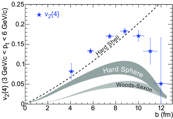
At higher , no longer rises with and the mass ordering is broken. Above GeV/c the more massive baryons exhibit a larger than the mesons. While the pion and kaon reach a similar maximum of at , the baryon continues to rise until it reaches a maximum of at GeV/c. For still larger , the values exhibit a gradual decline until for all particles is consistent with at GeV/c. Fine detail cannot yet be discerned at due to statistical and systematic uncertainties. At these higher values one expects that the dominant process giving rise to is jet-quenching[85] where hadron suppression is larger along the long axis of the overlap region than along the short axis[86, 87, 88]. For very large energy loss, the value of should be dominated by the geometry of the collision region. Fig. 16 shows a comparison of data[89] for GeV/c compared to several geometric models[90]. This comparison seems to indicate that in this intermediate range is still too large to be related exclusively to quenching.
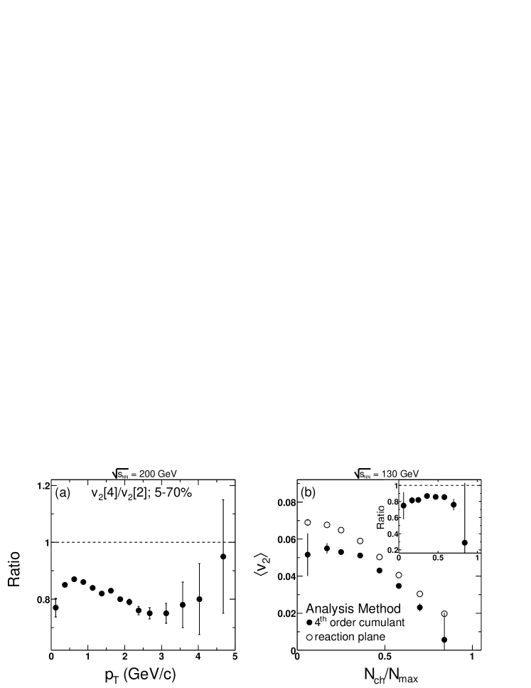
In the higher regions, significant azimuthal structure will arise from jets, so non-flow correlations are thought to be significant in this region[58]. These effects have been studied in several ways. The four-particle cumulant has been studied as a function of and the ratio of the four- and two-particle cumulants is found to decrease with increasing [92, 91]. This decrease is identified with a gradual increase in the contribution of jets to (see Fig. 17 left panel). The four-particle cumulant suppresses contributions due to intra-jet correlations but the statistical errors of the measurement are larger. One can also suppress jet structure in the measurement by implementing a cut in the pairs of particles being used in the analysis[11]. In this case, a high particle is correlated with other particles in the event that are separated by a minimum . This method relies on the assumption that jet correlations do not extend beyond a given range. Interactions of jets with the medium in nuclear collisions however can change the structure of jets and extend the correlations in beyond the widths observed in collisions[93]. This method therefore is not guaranteed to eliminate non-flow from jets. The problem of measuring without non-flow and of measuring modifications of jet structure by the medium are entirely coupled. If one is known, the other is trivial.
Other methods for suppressing non-flow include measuring correlations between particles at mid-rapidity and and an event-plane determined from particles observed at forward rapidity[94]. In the extreme and the most effective case, the event-plane was reconstructed from spectator neutrons in a Zero-Degree Calorimeter to measure of produced particles near . An extension of analyses based on the change in correlations across various rapidity intervals is the analysis of the two dimensional correlation landscape for two-particle correlations e.g. [95]. After unfolding the two particle correlations one can attempt to identify various structures with known physics such as jets, resonance decay, or HBT based on their width in and . The remaining structure can then be used to estimate . This method will be discussed below.
As we study progressively smaller systems the connection between the nucleus-nucleus reaction-plane and the azimuthal structure breaks down. In the limit that one proton from each nucleus participates in the interaction, the reaction-plane defined by the colliding protons will not necessarily be related to the reaction-plane defined by the vector connecting the centers of the colliding nuclei. In order to facilitate a comparison between the dependence of azimuthal correlations in large systems and small systems, the scalar product is used where and [89]. The mean of therefore yields a quantity that depends on and non-flow as follows:
| (5) |
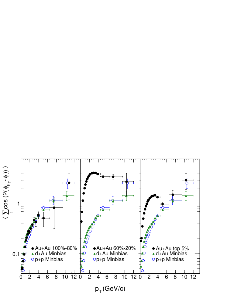
where is the multiplicity used in the sum. Fig. 18 shows this quantity for , Au, and three Au+Au centrality intervals. The and Au data are repeated in each of the panels. The most peripheral Au+Au collisions are shown in the left panel. The centrality bin shown is not usually presented since trigger inefficiencies for low multiplicity events makes it difficult to define the actual centrality range sampled. In this case, the data has been published in order to compare between the most peripheral sample of events and collisions. The data in Au+Au has a similar shape and magnitude as the data in . This suggests that peripheral collisions are dominated by the same azimuthal structure as collisions; an observation consistent with two-particle , correlations[96]. The data from mid-central Au+Au collisions shown in the middle panel however, exhibit a magnitude and shape clearly different than collisions. While for , Au and very peripheral Au+Au collisions rises monotonically with , for mid central Au+Au collisions, the data rises to a maximum at GeV/c and then falls. For central collisions shown in the right panel, a similar feature is seen with data rising to a maximum at GeV/c, then falling until GeV/c, where it begins rising again. This second rise is presumably a manifestation of non-flow at high in central collisions. These data suggest that azimuthal structure in Au+Au collisions above GeV/c is dominated by jets. This is also consistent with the conclusions reached by examining the particle type dependence of and [78].
In Fig. 18 the data is replotted in each panel to facilitate a comparison between the shape and magnitude in to that in Au+Au. In the absence of jet-quenching however, non-flow at high is expected to scale with the number binary nucleon-nucleon collisions . The plotting format in Fig. 18 on the other hand, assumes that rather than as would be expected for hard scattering. The multiplicity has been shown to scale as with [97, 98]. This is referred to as the two-component model. In order to compare azimuthal structure in Au+Au collisions to scaling of collisions we can form a ratio in analogy with for single hadrons:
| (6) |
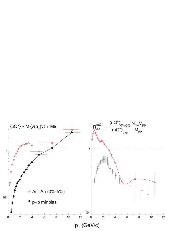
where and are the multiplicities in and collisions with taken according to the two component model. In the case that jet production in Au+Au collisions scales with the number of binary collisions, as hard processes are expected to, should be unity. The right panel of Fig. 19 shows for charged hadrons in central Au+Au collisions. For comparison, from single particle charged hadron spectra is also shown in the figure. first rises abruptly with to a maximum of 2 at GeV/c and then falls to a value of 0.25 at GeV/c. At GeV/c is similar to . This shows that jet-quenching suppresses the charged hadron spectra, and the azimuthal structure by a similar amount; confirming that the single hadron suppression is indeed related to jet-quenching. is complimentary to studies of , the ratio of dihadron correlations in Au+Au and collisions[57].
We note the presence of what appears to be a local minimum and local maximum and 2.0 GeV/c respectively. It is not clear if this is a real feature or simply an artifact largely caused by the shape of the data. In the case that it is a real feature, it is possibly related to the changing particle composition in Au+Au collisions where baryons with larger values become more prominent. At GeV/c, baryons and mesons in collisions are created in the proportion 1:3 while at the same in central Au+Au collisions the proportion is approximately 1:1. will be an interesting quantity to investigate for identified particles. One can anticipate a quark number dependence at intermediate as seen in and .
2.3 Multiply strange hadrons and heavy flavor
The build-up of space-momentum correlations throughout the collision evolution is cumulative. Information about space-momentum correlations developed during a Quark-Gluon-Plasma phase can be masked by interactions during a later hadronic phase. For studying a QGP phase, it is useful to use a probe that is less sensitive to the hadronic phase. Multi-strange hadrons have hadronic cross-sections smaller than the equivalent non-strange hadrons, and the values measured for hadrons such as -mesons () and -baryons () are therefore thought to be more sensitive to a quark-gluon-plasma phase than to a hadronic phase[32].
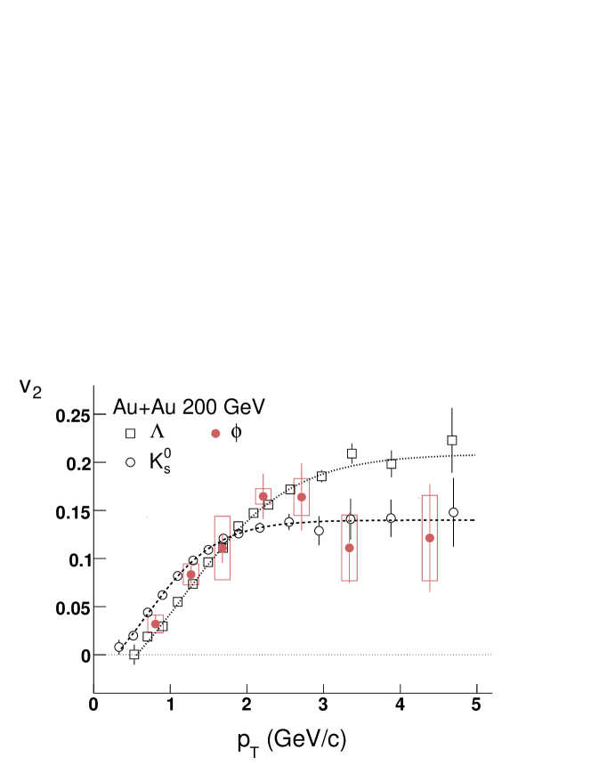
Fig. 20 shows for the -meson[99, 100]. The rises with and reaches a maximum of approximately at near 2 GeV/c. At intermediate , the -meson appears to follow a trend similar to the other meson . This observation suggests that either the -meson cross section is larger than anticipated or re-scattering during the hadronic phase does not contribute significantly to . The latter possibility requires that is established prior to a hadronic phase, suggestive of development of during a QGP phase.
Measurements of multiply strange hadrons are interesting because they should be less coupled to the matter in a hadronic phase and therefore a better reflection of the QGP phase. Heavy quarks on the other hand (e.g. charm and bottom quarks) may be less coupled to even the QGP matter[101, 102]. It’s not a priori obvious that heavy quarks will couple significantly to the medium and be influenced by its apparent expansion. The extent to which they do couple to the medium should be reflected in how large for heavy flavor hadrons becomes and how much the nuclear modification () deviates from unity. Precision measurements of Heavy Flavor mesons or baryons are not yet available from the RHIC experiments. As a proxy for identifying D-mesons, the STAR and PHENIX experiments have measured non-photonic electrons[103, 104]. Non-photonic electrons are generated from the weak-decays of heavy flavor hadrons and after various backgrounds have been accounted for can, with some caveats[105], be used to infer the and of D-mesons.
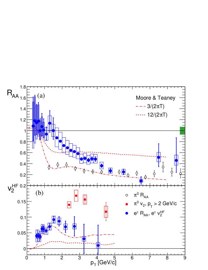
The top panel (a) of Fig. 21 shows for non-photonic electrons[106, 107]. Prior to the measurement of non-photonic electron , it was expected that heavy-flavor hadrons would be significantly less suppressed than light flavor hadrons. These expectations based on a decrease in the coupling of charm quarks to the medium because of the dead-cone effect[101], are contradicted by the data; At GeV/c, non-photonic electrons are as suppressed as pions. This suppression suggests a stronger than expected coupling of charm quarks to the medium. This coupling apparently also leads to significant as seen in Fig. 21 (b).
Also shown in the figure is a calculation of and based on a Langevin model[108]. In that model, the strength of the energy loss and momentum diffusion of charm quarks is characterized in terms of a diffusion coefficient (D). and for charm quarks is then computed for several values of D. Two of these values are shown in Fig. 21. Although neither curve provides an entirely satisfactory simultaneous description of and , the comparison suggests that the diffusion coefficient is large. This comparison only achieves rough agreement, but the calculation illustrates the sensitivity of heavy flavor hadrons to transport coefficients of the QGP and is an important quantity to measure for these hadrons. This is also in agreement with H. van Hees, et al.[109] where coalescence at the hadronization phase boundary is also considered and found to help improve the agreement with data.
2.4 Fluctuations and Correlations
Comparisons between data and models are complicated by uncertainties in the initial eccentricity and by uncertainties in the data. Estimating transport quantities from the data may require a precision comparison between eccentricity and so it is important to reduce the uncertainties in both. As discussed in the previous sections, a CGC model of the initial conditions yields eccentricity values typically larger than a Gluaber model while the fluctuations () are still of the same width. The ratio of in a CGC model is therefore smaller than in a Glauber model[65, 66]. One can expect the statistical fluctuations in eccentricity to show up as dynamical fluctuations in measurements. Measuring the dynamic fluctuations in conjunction with can therefore provide an additional constraint on the initial conditions[110, 111, 112, 113].
Several methods have been employed for measuring and the various methods have different dependencies on non-flow correlations and fluctuations[68, 114, 115, 116, 71, 59, 117, 118]. The differences between these measurements give information on non-flow correlations and fluctuations. If one uses a two particle correlation to estimate , then one finds where the average is over all unique pairs of particles. is the single particle anisotropy with respect to the reaction plane and is the non-flow parameter which summarizes the contributions to from correlations not related to the reaction plane. If one uses a 4-particle cumulant calculation, then for most cases the non-flow term will be suppressed by large combinatorial factors and fluctuations will contribute with the opposite sign. For Gaussian fluctuations, [71]. Without knowing or , one cannot determine the exact value of . Rather, could lie anywhere between and .
It is advantageous to confront various models with the data that is experimentally accessible. The difference between the two- and four-particle cumulants in the case of Gaussian fluctuations is:
| (7) |
The term is also approximately equivalent to the non-statistical width of the distribution of the length of the flow vector distribution and is called . The flow vector for the harmonic is defined as and . Fig. 22 shows extracted from the difference between the two- and four-particle cumulants[11]. In the case of Gaussian fluctuations, higher cumulants such as are equal to . In this case, the quantity and summarizes the information available experimentally from the second harmonic flow vector distribution. No more information can be accessed without applying more differential techniques or by making assumptions about the shape or centrality dependence of flow, non-flow, or flow fluctuations. An example of a more differential analysis is also shown in Fig. 22, where two particle correlations have been fit in - space[119]. Terms identified with various non-flow sources have been included with the fit and the remaining modulation is then identified as . In the case that the sources of non-flow are correctly parametrized, , where is integrated over all azimuthal structure. Then . This procedure is discussed below.
Even without attempting to disentangle flow fluctuations from non-flow correlations, the assumption that non-flow is a positive quantity (consistent with ) can be used with to provide an upper limit on fluctuations
| (8) |
To facilitate a comparison between this limit and models of the initial eccentricity the upper limit on is compared to in the model. To form this ratio appropriately, the same assumptions should be made for and i.e. zero non-flow.
| (9) |
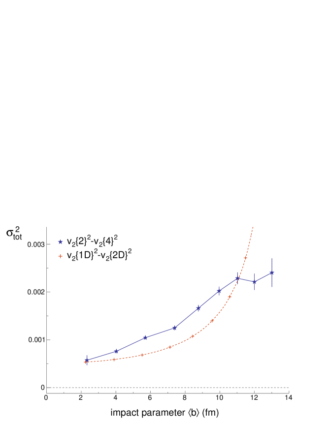
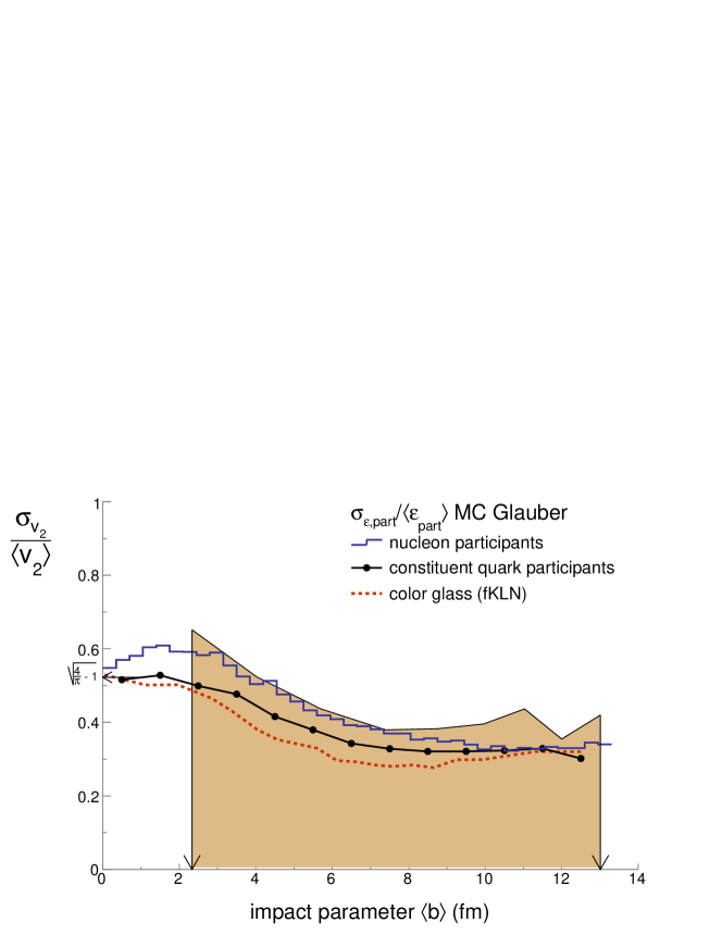
This upper limit is shown in Fig. 23 and compared to several models of . The models include two Glauber Monte Carlo models[121]; one using the coordinates of participating nucleons to calculate the eccentricity, the other using the coordinates of constituent quarks confined inside the nucleons. The constituent quark Monte Carlo Glauber Model (cqMCG)[112] treats the nucleus as constituent quarks grouped in clusters of three confined to the size of a hadron. This increases the number of participants by roughly a factor of three, reducing the fluctuations in eccentricity. The correlations between the constituent quarks required by confinement partially counteract this effect since those correlations act to broaden the eccentricity distribution. The net effect, however, is a narrowing of the distribution. Also shown is a Color Glass Condensate (CGC) based model which yields eccentricity values 30% larger than the Glauber models leading to a reduction of . The Monte Carlo Glauber model based on the eccentricity of nucleons already exhausts most of the width . This shows that the statistical width of the eccentricity fluctuations in the Glauber model already accounts for almost all of the non-statistical width of the flow vector distribution thus leaving little room for other sources of fluctuations and correlations. This is particularly challenging since non-flow has been neglected in setting the upper limit and the only fluctuations considered are those arising from eccentricity fluctuations. We have therefore neglected fluctuations that would arise during the expansion phase[120, 122, 119]. One can write the total width including these terms:
| (10) |
where the middle term in the right-hand-side is the fluctuations from eccentricity fluctuations and the final term is fluctuations from the expansion phase. The middle term arises from the approximation that to first order . This approximation is prevalent in the literature. The last term can be related to the Knudsen number of the matter during the expansion[122]. Measurements demonstrating the existence of non-flow or dynamic fluctuations () therefore would challenge the model. The CGC or cqMCG models provide a more likely description since is smaller in those models than the upper limit on . The upper limit on provided by provides a valuable test, therefore, for models of the initial eccentricity and can help to reduce the uncertainty on ; an essential component in extracting meaning from the value of .
2.4.1 Two Dimensional Correlations and


One way to study non-flow contributions to two-particle correlations is to measure the correlations as a function of and [95]. This allows different sources of two particle correlations to be studied where each source is identified by its characteristic dependence on and . Additional information can be obtained by including information about the charge-sign dependence of the correlations. An example of such an analysis is shown in Fig. 24. The figure displays four panels. The top panels show the correlation density
| (11) |
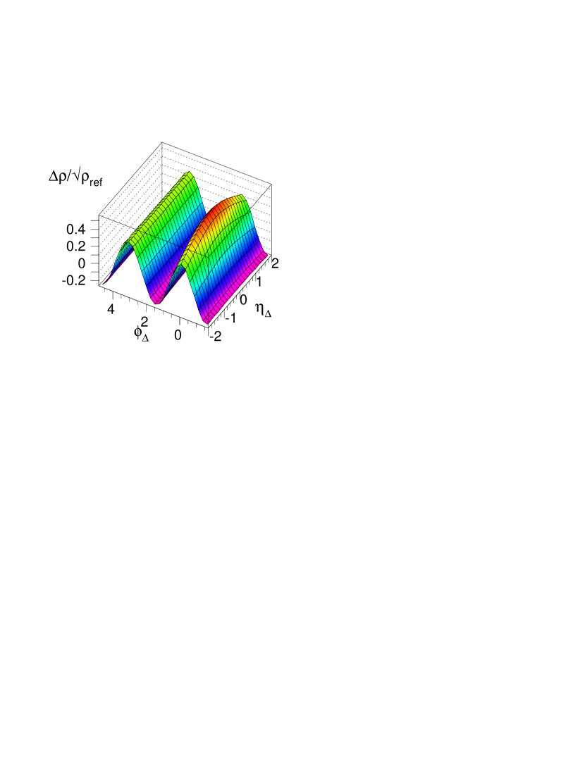
where is the pair density and is the product of the single particle densities. This normalization is chosen to search for deviations of the correlations in large systems from those in small systems. If Au+Au collision were simply a superposition of collisions for example, would be the same in and Au+Au collisions. This figure was produced based on simulated data which was tuned to match real data in very peripheral Au+Au or collisions (top left) and 20%-30% central Au+Au collisions (top right)[119, 123]. The correlations in these two systems have been found to be very different. The collisions exhibit structures characteristic of fragments from string breaking (a narrow ridge at independent of ) and fragments from semi-hard scattered partons or mini-jets. These mini-jets yield a two-dimensional Gaussian correlation at , and a broad ridge at . The away-side jet can sweep over a wide range since the partons can have a momentum within the proton or Au nucleus. For semi-central and central Au+Au collisions, the correlation landscape is drastically different with the most prominent feature being giving rise to a clear shape. If the shape of the various non-flow terms structures is well understood, the correlation landscape can be fit and can be extracted, independent of the sources of non-flow. This procedure depends on having an accurate description of the shape of the non-flow sources. Some of these are easily identified based on their charge dependence or their characteristic shapes. Other sources may be less easily identifiable though, particularly if they become modified by the medium in Au+Au collisions.
The bottom panels of Fig. 24 show a proof-of-principle extraction of based on the simulated data. The left panel shows while the right panel shows the per-particle measure . Also shown are the two-particle and four-particle cumulant data. The upper hatched region in the bottom left panel shows
| (12) |
extracted without separating out non-flow; called . is the multiplicity of measured tracks. The lower hatched region shows the same without including the non-flow structures in the calculation; called . Data are plotted versus so that most central collisions are on the right. This procedure makes use of the two-particle correlations landscape to separate different contributions to the azimuthal structure. The fit procedure does require some assumptions be made in order to separate non-flow from [123]. These include that and are independent of and that higher harmonics of and do not contribute. Relaxing those assumptions may make it difficult to distinguish between non-flow and more complicated correlations related to the reaction plane. More information can be made use of however, by examining the charge, sign dependence and particle-type dependence of the various correlation structures. This is therefore a promising method for disentangling and non-flow.
2.5 Scaling Observations
Elliptic flow measurements represent an extensive data set. has been measured for GeV/c, for , for mesons from the pion to the and , for baryons from the proton to the , and for transverse particle densities . And yet, given the complexity of heavy-ion collisions and such a large data-set, the measurements exhibit many surprisingly simple features. These we can summarize in terms of simple scaling observations where a large amount of data is found to behave in a regular and simple way when plotted versus the appropriate variable. The observation of a particular scaling then motivates the question: why does the data only depend on that variable? These scaling observations, therefore, not only allow us to summarize large amounts of data in a simple form, but they also suggest simple physical explanations for the data with perhaps deeper implications. In this section I review several observed scaling laws.
2.5.1 Longitudinal scaling
Fig. 12 shows the centrality dependence of [75]. Although more detailed measurements at small show that is approximately independent of for [11], the data extending to larger exhibit a nearly triangular shape: having a maximum at with a nearly linear decrease with . A similar shape is seen for 200, 130, 62.4, and 19.6 GeV Au+Au collisions[124].
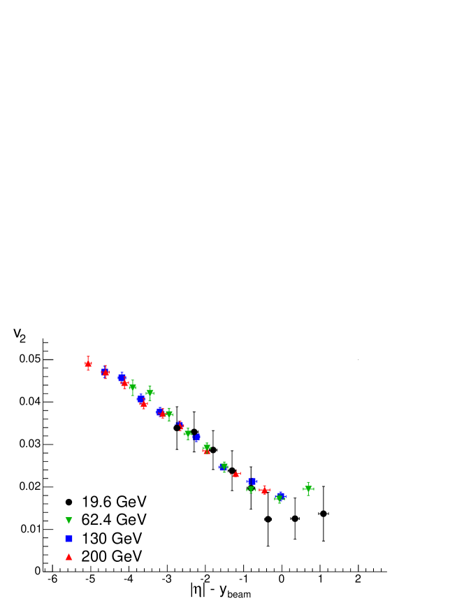
Fig. 25 shows for from 19.6 to 200 GeV; one order of magnitude in . The data are for the 40% most central collisions. Ideally the x-axis would display but data on identified particle spanning such a large range of rapidity are not available. One finds that within errors, all data lie on a single curve. This suggests a smooth variation of the development of space-momentum correlations from forward rapidity to mid-rapidity. This scaling observation also implies that the value of obtained at mid-rapidity is a smooth function of or equivalently of ; consistent with the smooth trend seen in Fig. 3 for above of approximately 5-10 GeV. An energy scan at RHIC extending down to GeV will make it possible to investigate this trend with better precision and with a single detector, eliminating many systematic uncertainties[125]. This simple trend may be confirmed with more precision or perhaps deviations will point to a softest point in the equation-of-state[126, 127].
2.5.2 Kinetic Energy and Constituent Quark Number Scaling
At low , is ordered by mass with heavier particles having a smaller value at a given value[76, 77]. This ordering is indicative of particle emission from a boosted source with the boost larger in the in-plane direction than the out-of-plane direction. Indeed, blast-wave fits implementing this scenario agree very well with the data in this region[47]. It is also found that in this same region, when is plotted versus all data fall on a common line[128]. is the particles transverse kinetic energy and sometimes labeled KET[129]
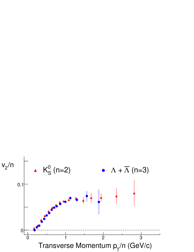
Fig. 26 shows versus for particles ranging in mass from the pion with mass of 0.1396 GeV/c2 to the with mass of 1.321 GeV/c2. The measurement is made for the 0-80% centrality interval in 200 GeV Au+Au collisions. Similar scaling has also been demonstrated for 62.4 GeV collisions[81]. The data exhibit obvious trends. At low , values for all particles rise linearly with no apparent differences between the particles with different masses. Near GeV/c2, for mesons and baryons diverges. The meson begins to saturate, obtaining a maximum value of 14-15% near GeV/c2. The baryon continues to rise, obtaining a maximum value of approximately 19-20% at to 3.5 GeV/c2. The relative masses of the baryons and mesons do not seem to be relevant, rather the number of constituent quarks in the hadron determines the values in this range. The mass dependence can be better checked using the -meson which has a mass slightly larger than that of the proton. The statistical significance of the is limited but measurements seem to indicate that the lies closer to the mesons than to the baryons i.e. closer to the particles with a common number of constituent quarks than to particles with a common mass[99].
The observation of the quark-number dependence of at intermediate led to speculation that hadron formation through the coalescence of dressed quarks at the hadronization phase boundary could lead to an amplification of with baryons getting amplified by a factor of 3 while mesons were amplified by a factor of 2[130, 131, 132, 140, 133, 134, 135, 136, 137, 138, 139, 140]. This picture was subsequently strengthened by the observation that a similar quark-number dependence arises in [78, 141]: the ratio of the single particle spectra in central collisions to that in peripheral collisions. At intermediate the values for various particle species are also grouped by the number of constituent quarks, with baryons having a larger . The larger for baryons signifies that baryon production increases with collision centrality faster than meson production; an observation consistent with the speculation that hadrons from Au+Au collisions are formed by coalescence such that baryon production becomes easier as the density of the system increases. The more general and less model dependent statement is that the baryon versus meson dependence arises from high density and therefore most likely from multi-quark or gluon effects or sometimes called” higher twist” effects. The combination of large baryon and large baryon also immediately eliminates a class of explanations attempting to describe one or the other observation: e.g. originally it was speculated that the larger for baryons might be related to a smaller jet-quenching for jets that fragment to baryons than for jets that fragment to mesons. This explanation would lead to a smaller baryon and is therefore ruled out by the larger for baryons. The same can be said for color transparency models[142] which would account for the larger baryon in this region but would predict a smaller baryon . Color transparency may still be relevant to the particle type dependencies at where for protons is slightly larger than for pions[143] and the measurements are not yet precise enough to conclude whether the baryon is also smaller than the meson . This is a topic that needs to be studied further.
In a coalescence picture, the final momentum of the observed hadron would depend on the momentum of the coalescing constituent quarks. The exact dependence is not known but a relatively good scaling of for and was found when was plotted as a function of . Such a scaling implies that the momentum of the hadron is simply the sum of the momenta of the coalescing quarks. Fig. 27 shows versus for -mesons and -baryons. The scaling appears to be good throughout the whole range but part of this perception is due to the decrease of for both particles at small . When a ratio is taken between the values, a clear deviation from scaling is seen in the lower region. A combination of the scaling in Fig. 26 and the scaling in Fig. 27 will lead to a good scaling over the whole measured momentum range; since for all particles fall on a single line at low , dividing the x- and y-axis by n will not destroy that scaling seen in Fig. 26. Plotting versus should therefore provide a good scaling across a large kinematic range.
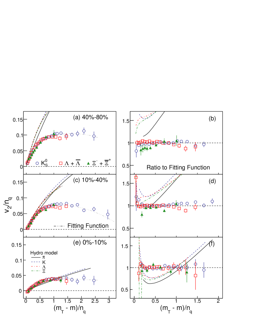
Fig. 28 shows versus for 200 GeV Au+Au collisions in three different centrality intervals[80]. Data for -mesons, -baryons and -baryons are shown. The left panels show the data with a hydrodynamic calculation and a fitting function. The phenomenologically motivated function
| (13) |
with , describes the data well for the three centralities. The function captures the rise then saturation and steady decline seen in the data. We ascribe no physical meaning to the function or the five fit parameters but simply use it as a convenient reference. The right panels show the ratio of the data and the hydro model to the fit function. For reference, the fit parameters are shown in Table 1. The data is in good agreement with the fit function for all centralities while this hydro model calculation does not agree well with the data in any centrality.
| Fit parameters for Eq. 13 | |||||
| Centrality | a | b | c | d | e |
|---|---|---|---|---|---|
| \colrule40%-80% | 20.0e-02 | 0.0 | 0.0 | -1.19e-02 | 2.37e-01 |
| 10%-40% | 16.4e-02 | -4.53e-03 | 0.0 | 2.61e-02 | 2.40e-01 |
| 0%-10% | 8.96e-02 | -4.08e-03 | 0.0 | 6.52e-02 | 2.70e-01 |
There is a systematic deviation from the ideal n scaling at GeV/c2 with mesons having slightly larger values than baryons. This deviation from ideal scaling was predicted based on the inclusion of higher fock states in the hadrons or the inclusion of a finite width in the hadron wave function[144, 145]. Deviations can also arise in a hadronic phase when the hadronic cross sections are relevant. In the case that hadronic cross-sections are an important factor, higher statistics data for baryons and mesons should deviate from their respective groups. We also note that hadronic cascade models also obtain approximate scaling due to the use of the additive quark model for hadronic cross-sections[146]. On the other hand, these models under-predict the integrated by a factor of two. We also note that non-flow contributions can affect the scaling observed in this range and the particle-type dependence of non-flow sources is still being investigated.
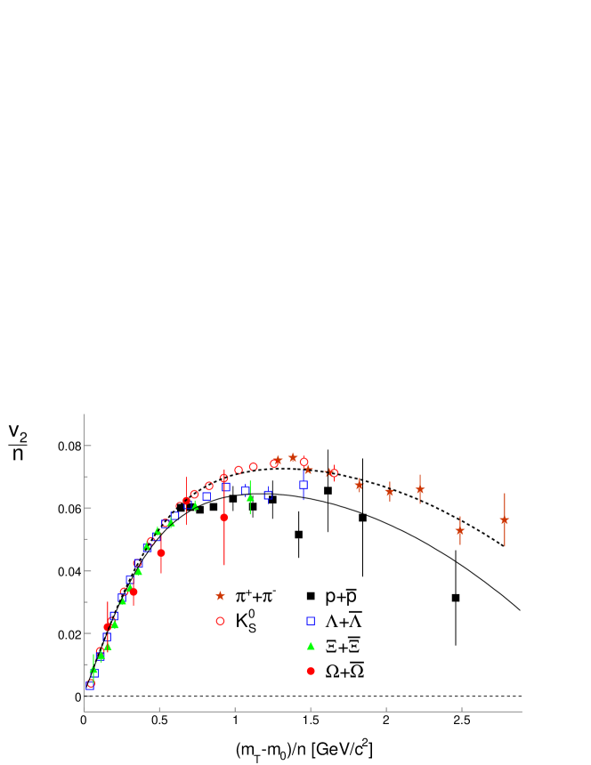
In Fig. 29 we investigate the breaking of ideal scaling in more detail with data integrated over a larger centrality interval. While this reduces the statistical uncertainty, it also introduces uncertainties due to the large centrality bin width. In particular, when particle yields have different centrality dependencies, the average eccentricity of events producing a particle can deviate from particle to particle. For example, the enhancement of baryons in central collisions will mean that the average baryon comes from a more central event than the average meson. Given the decrease of with centrality, this can lead to a decrease of baryon simply due to the wide centrality bin. Although there are caveats and systematic errors still to be quantified, we note that the baryons in Fig. 29 appear to lie systematically and significantly below the mesons. Self-similar curves are fit to mesons and baryons. The curves appear to describe the data. We note that the two self-similar curves shown in Fig. 29 can be nearly unified if we replace n with n+1. This demonstrates that the naive constituent quark scaling is violated to the extent that baryon is actually closer to 4/3 the meson rather than 3/2. The connection of the baryon versus meson dependence and the number of constituent quark scaling appears to not be as directly connected to the number of constituent quarks as originally conceived. Whether this is indicative of higher fock states, the wave-function of the hadrons, an as yet un-accounted for experimental systematic error, or something else is yet to be determined. The systematic uncertainties based on the particle-type dependence of non-flow are still being investigated.
2.5.3 System-Size Scaling
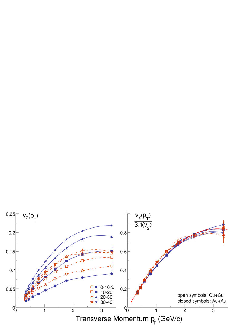
The system-size dependence of can be studied by looking at the centrality dependence of or by colliding smaller nuclei. Ideal hydro predictions, having a zero mean-free-path assumption, should be independent of the system-size. In this case, given the same eccentricity, the should be independent of system size. One can try to account for the change in eccentricity by dividing by eccentricity from a model but this introduces a large amount of uncertainty. Another approach is to study the shape of to see if that varies[147]. The left panel of Fig. 30 shows measured in Au+Au and Cu+Cu collisions for several centrality intervals[129]. In the right panel, is scaled by 3.1 times the mean for that data set. was taken as a proxy for the eccentricity of the collision system, and this proxy is not inconsistent with models of eccentricity which are quite uncertain. What is best demonstrated by this scaling, is that although the magnitude of changes significantly for the different centralities and systems, the shape of is very similar.
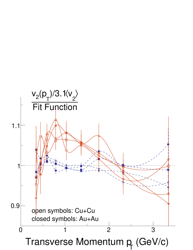
The invariance of with system-size can be taken as an indication that the viscosity of the expanding medium created in heavy-ion collisions can not be large when is established; Large viscous effects should introduce a system-size dependence to with viscosity causing to saturate at lower values in the smaller system[147]. Hydrodynamic calculations including viscosity confirm this idea[148, 149, 150, 151, 152, 153]. To look more carefully for a system-size dependence in the shape of we plot the ratio of the scaled data to a curve fit to the Au+Au data. The results are shown in Fig. 31. The Cu+Cu data systematically deviate from the Au+Au data. The dependence of the ratio indicates that the Cu+Cu data begins to saturate before the Au+Au data. This leads to a ratio that first rises then falls. This would happen the other way around if the Au+Au data saturated first. The uncertainties in the figure are large but the shapes are still significantly different. The system-size dependence of may be a valuable tool for estimating the viscosity of the matter created in heavy-ion collisions.
Although the data on includes many particle types, a wide kinematic range in and , a variety of system-sizes and a wide range in center-of-mass energy, we’ve been able to identify several regular features of the data. These include a nearly linear rise of at mid-rapidity with :
| (14) |
for 0%-20% central Au+Au or Pb+Pb collisions and a , mass and particle-type dependence that can be parametrized by
| (15) |
where , while to good approximation decreases linearly from it’s maximum at mid rapidity to beam rapidity. This linear rise may be a trivial consequence of the dependence of mid-rapidity or vice-versa.
3 Confronting the Hydrodynamic Paradigm with RHIC Data
We have discussed the hydrodynamic model extensively in this review as a convenient reference for how well the matter produced in heavy-ion collision converts spatial deformation into momentum space anisotropy. Hydrodynamic models of heavy-ion collisions have many uncertainties. These include, uncertain initial conditions, uncertain thermalization times, and uncertain freeze-out conditions. A successful description of data using a hydrodynamic model offers the promise of not only establishing the attainment of local equilibrium but also the promise of providing information on the Equation-of-State of the matter and its transport properties. The uncertainty in the models, however, are large and it has not yet been possible to extract this desired information with satisfactory certainty. In addition, the possibility that significant arises from initial-state effects[37, 34] could call into question the applicability of hydrodynamics and the need for prolific final-state rescattering. Measurements of two particle correlations, which have often been interpreted as arising from mini-jets[96, 119], need to be reconciled with the idea of a locally thermalized matter with extensive final-state rescattering. If the hydrodynamic models and data are irreconcilable, the paradigm will, of course, have to be abandoned.
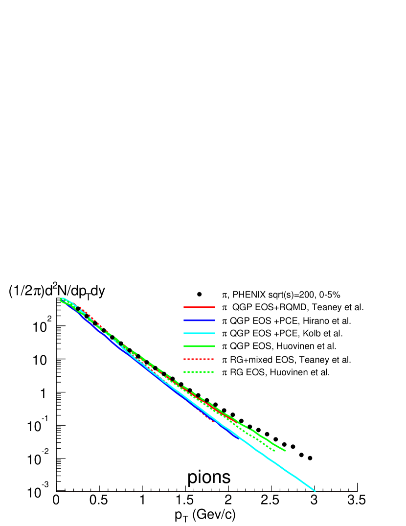
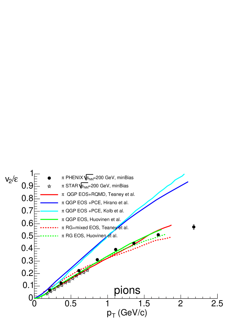
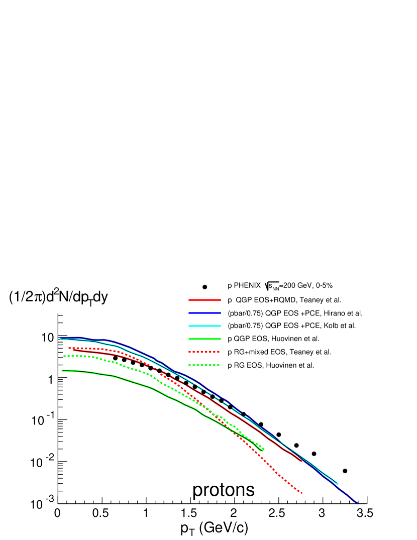
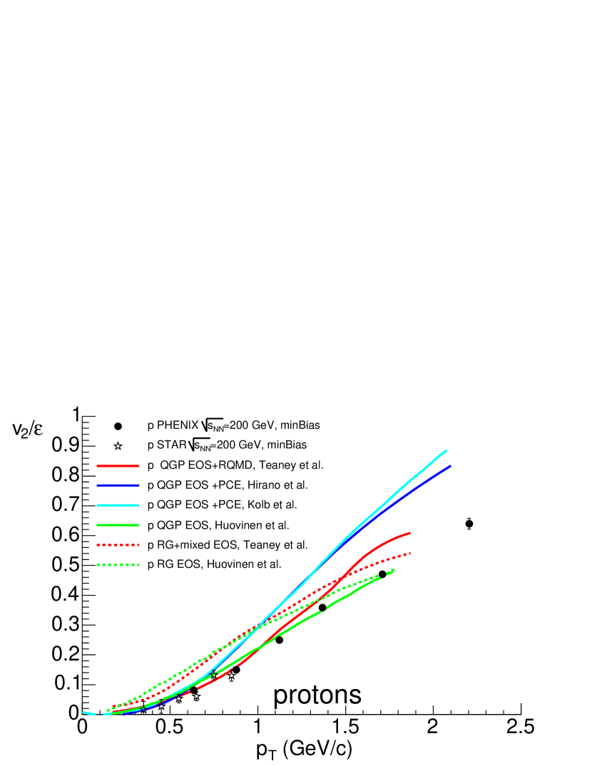
To check for consistency with hydrodynamic models[29, 30, 154, 155, 156], the PHENIX collaboration created a comprehensive comparison between heavy-ion data on spectra and [8]. The inclusion of a comparison to HBT data was hampered by the lack of predictions from some of the models. The comparison to spectra and is shown in Fig. 32. The left panels show spectra with pions in the top panel and protons in the bottom. The right panels show for the same particles. The combination of data on and spectra provide a stringent test for the models as some models can reproduce one quantity but only by adjusting parameters in such a way that the agreement with other observables is spoiled.
The models shown in the figure differ in several ways. Models that include a phase transition and a QGP phase are shown with solid lines while models without a pure QGP phase are shown as dotted lines. Including this phase transition acts to reduce the value of since the equation of state is soft during the transition. This means that the speed of sound drops (in these models to zero), so that conversion of coordinate space eccentricity to momentum space anisotropy is halted during the phase transition. In the case that the models, do approximately match the pion spectra and , the most directly observable consequence of the lack of a phase transition is on the proton spectra and proton . The proton spectra end up being too soft, and the splitting between proton and pion is reduced with the proton becoming larger. This is somewhat counter-intuitive but is a consequence of fixing the parameters to match central data.
The models also differ in their treatments of the final hadronic stage. The calculations from Teaney et al. include a hybrid model that uses a hadronic cascade (RQMD) for the final hadronic evolution. Hirano and Kolb do not use such an afterburner but allow the particle abundances to stop changing at a temperature above the temperature at which they stop interacting; chemical freeze-out happens before kinetic freeze-out. Huovinen on the other hand, maintains chemical and kinetic equilibrium throughout the expansion. These different treatments have very important consequences for the particle-type dependence of the spectra and . Huovinen’s treatment can reproduce the for pions and protons, but only at the expense of under-predicting the number of protons; a direct consequence of maintaining chemical equilibrium until the final freeze-out at a relatively low temperature.
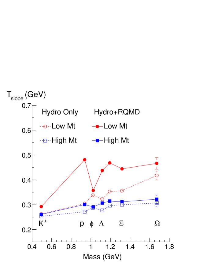
The only model which compares well to all the data is Teaney’s model including a QGP phase, a phase transition, and a hadronic phase modeled with RQMD. Such a hybrid model adds significantly to the number of tunable parameters as compared for example to Huovinen’s model. On the other hand, the Teaney model shows that some particle types are less affected by the hadronic phase and therefore less sensitive to some of the uncertainty in freeze-out prescription. Fig. 33 shows the Teaney calculation with Hydro only versus Hydro+RQMD. The particle species least affected by the inclusion of a hadronic afterburner, are the -meson and the -baryon. This arises presumably from the small hadronic cross-section for these hadrons. This suggests high-statistics measurements for these particles are a viable way to avoid uncertainties in the effects of hadronic re-scattering.
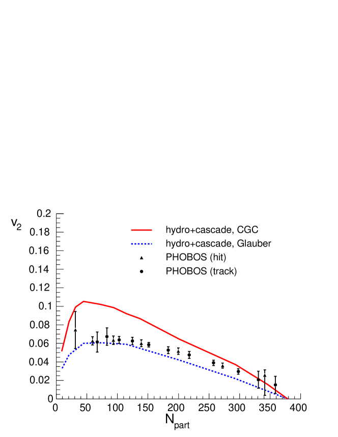
Besides the uncertainty in the freeze-out prescription, there is uncertainty on the eccentricity of the expanding fire-ball at the start of the conjectured hydrodynamic evolution. Fig. 34 shows a hybrid hydro+cascade model compared to data[72]. Two model curves are shown: one with a Color-Glass-Condensate (CGC) initial eccentricity[66], the other with a Monte-Carlo-Glauber (MCG) eccentricity. As discussed previously the CGC eccentricity is larger than the MCG eccentricity; this leads to an over-prediction for . On the other hand, this hybrid model does not include viscous effects in the QGP phase so the difference between the hybrid+CGC prediction could be related to viscosity. In fact, since viscosity acts to reduce , the hybrid+MCG curve shows that there is no room for viscosity in this model. This violates the lower bound on viscosity derived based on quantum mechanical arguments[158] and also later from string theory[159]. Clearly, to estimate the viscosity allowed, or required by the data, the uncertainty on the initial conditions must be reduced. As discussed previously, the measured quantity provides a sensitive test of the models of the initial conditions and needs to be carefully compared to the hydrodynamic model predictions with various initial conditions.
3.0.1 Transport Model Fits
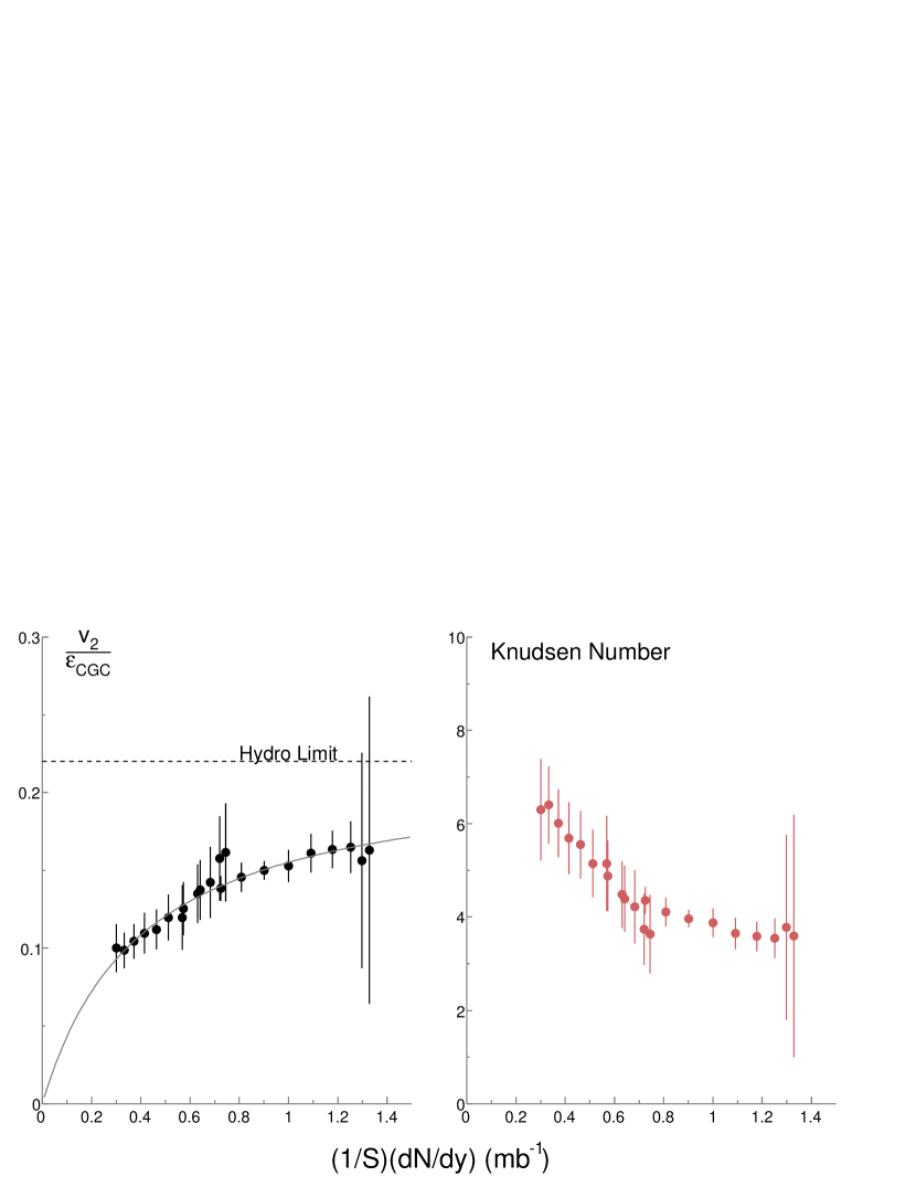
An approach to circumvent the uncertainties in the hydrodynamic models has been outlined in Ref.[160, 161] where is fit as a function of . The fit function is used to infer how close the data come to a saturated value in the collisions with the highest density achieved. The fit function is constrained by how should approach the high density and the low density limits. One can construct different equations but in a transport code, the following was found to represent the approach to the zero mean-free-path limit well[162]:
| (16) |
where is the Knudsen number and is a constant of order one. Fig. 35 shows the data and fit in the left panel and the inferred Knudsen number in the right panel. Based on this procedure it is found that RHIC data are still some 20% below the saturation value anticipated within the fit function. This conclusion however, not only depends on the assumptions built into the transport model approach but also the centrality dependence of the eccentricity. The Color Glass Condensate model for example predicts a stronger centrality dependence for the eccentricity than the Monte Carlo Glauber model. As a consequence, this fit implies that if the initial conditions at RHIC are described by the CGC model, then the data is closer to its saturation limit than if the MCG gives the correct description. This is counter intuitive and opposite to the conclusions reached based on real hydrodynamic calculations, which indicate that the larger CGC initial eccentricity allows more room for viscous effects in the QGP phase[148, 150]. The transport based fit circumvents the actual solving of hydrodynamics but the conclusions are dependent on the centrality dependence of the initial eccentricity which is strongly model dependent. The fit also includes the speed of sound as a free parameter. This effectively leads to an equation of state which has no phase transition but which is allowed to vary in the fit. A complimentary and perhaps better method for accessing the Knudsen number and the viscosity is to study the shape change of for different system-sizes which avoids the uncertainty in the eccentricity[147]. This is a work currently in progress.
3.0.2 Viscous Hydrodynamics
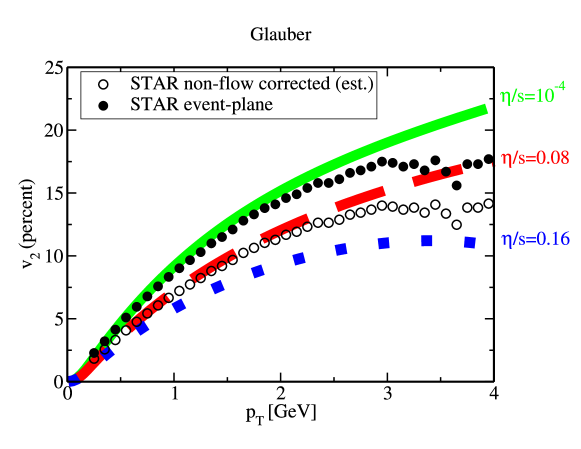
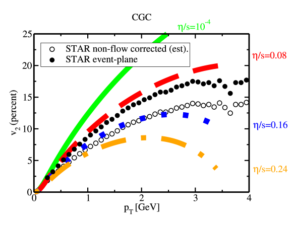
The apparent success of ideal hydrodynamic models to describe the gross features of RHIC data has led to the inference of small viscosity and the claim of the discovery of the perfect liquid at RHIC. The perfect liquid announcement was listed as the top physics story of 2005 by the American Institute of Physics and was widely covered in the popular press. Much recent work has gone towards including viscous effects in hydrodynamic calculations so that the viscosity can be more accurately estimated[148, 149, 150, 151, 152, 153]. Fig. 36 shows one such calculation. The top panel shows results when the hydrodynamic evolution starts from Glauber initial conditions while the bottom panel shows the case of CGC initial conditions. The results that come closest to the STAR data[81] are given by for the Glauber initial conditions and for the CGC initial conditions. The STAR non-flow corrected data are from Figure 4 of Ref.[80]. The 10%-40% central data from that reference was scaled to account for the difference between the 10%-40% centrality interval and the 0%-80% (minbias) centrality interval. The larger inferred based on the CGC model arises from the larger initial eccentricity which leaves more room for viscous effects that tend to reduce the . This contradicts the conclusions drawn from the transport model inspired fit, which allows the equation-of-state to change for the two different initial conditions. The dependence of the data is also better captured in the larger viscosity CGC scenario. The larger viscosity inferred from the CGC initial conditions gives a more pronounced turn over of which better describes the dependence of . The comparison shown in Fig. 36 shows that hydrodynamic models including viscosity have a good chance of reproducing RHIC data as long as the shear viscosity to entropy ratio is less than where is the conjectured lower limit.
3.0.3 Fluctuating Initial Conditions
The comparison of and other RHIC data to hydrodynamic models seems to indicate that when viscous corrections are included, a successful description of the data may be possible. There is uncertainty in this comparison, however, related to uncertainties in the initial conditions and in the freeze-out prescription. The uncertainty in the initial conditions can be addressed experimentally with measurements of fluctuations which in turn require an understanding of non-flow correlations; The experimentally accessible information appears to reduce to and . An alternative approach may be for hydrodynamic models to predict and by including correlations and fluctuations in the models. Progress has been made in this direction. Early work relating to the effect of fluctuations in the initial conditions on hydrodynamic calculations was carried out using the NeXSPheRIO hydrodynamic model[67, 163]. The initial eccentricity fluctuations were indeed found to lead to fluctuations as shown in Fig. 37. Later it was suggested that correlations in the initial conditions could lead to fluctuations of even and odd orders of that would manifest themselves as non-sinusoidal, apparently non-trivial, two-particle correlations as seen in the RHIC data[69, 164].
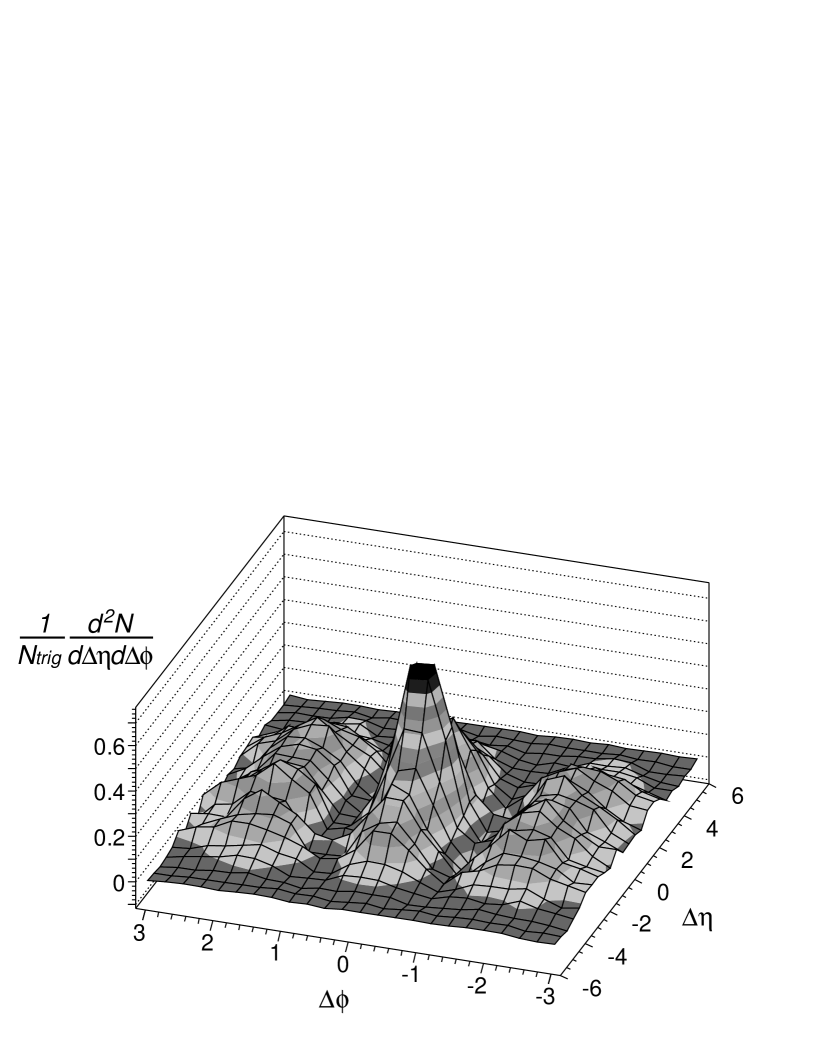
Subsequent work following through on this idea shows that hydrodynamic models with fluctuating initial conditions do lead to two-particle correlations with structure beyond a simple shape[165]. The correlation structure arising from the fluctuations in the initial conditions is shown in the right panel of Fig. 37. The model exhibits many of the features seen in the data including a jet-like peak, a near-side ridge, and an away-side ridge shifted away from . All this structure arises without the explicit inclusion of jets in the model. The apparently exotic correlations do not appear in the model when a smooth initial condition is used. This calculation illustrates the importance of accounting for fluctuations in the initial conditions when interpreting the correlation landscape. It also demonstrates that complex interactions between jets and the medium, including mach-cones, are not needed to explain the correlations data nor is the concept of mini-jets necessarily required.
In light of the NeXSPheRIO calculations, the highly structured correlation landscape at RHIC should not necessarily be taken as an invalidation of the hydrodynamic models. The correlations may simply reflect the need to abandon certain approximations, including the approximation of infinitely smooth initial conditions. Besides comparing to two-particle correlation data, these models can be used to calculate and to directly compare to data. It will be interesting to see how the correlation landscape in this model depends on the parameters of the model, in particular, the thermalization time and the freeze-out time. The connection of fluctuations (related to two-particle correlations) to the lifetime of the system was first pointed out by Mishra et al.[166]. In that reference the authors also introduce the anaology between fluctuations and the power spectrum of the Cosmic Microwave Background Radiation.

3.0.4 Addressing Uncertainties
Uncertainties in the freeze-out prescription and the effects of the hadronic phase can be experimentally addressed through precise measurements of -mesons and -baryons. Models indicate that due to their small hadronic cross-sections, these hadrons are minimally influenced by the hadronic phase and reflect well the QGP phase. In addition, heavy flavor hadrons may help determine or provide a cross-check for the transport properties of the QGP. Another approach to extracting the viscosity is by studying the shape of versus system size. This approach does not rely on a model for the initial eccentricity. Uncertainties in the eccentricity and the initial conditions can be reduced through measurements of fluctuations and two-particle correlations. These studies are ongoing. One can also measure fluctuations for arbitrary value. These are of course related to the two-particle correlation landscape which has already been extensively studied at RHIC. It will be of great interest to see how the correlation landscape predicted in hydrodynamic models with fluctuating initial conditions changes depending on the model parameters. The correlations data may help constrain quanties like the lifetime of the system. The studies listed above, along with a beam-energy scan at RHIC and the first data from LHC, will allow for more progress in understanding the matter created in heavy-ion collisions and its subsequent evolution.
4 Summary
In this review, measurements were presented as a method for studying space-momentum correlations in heavy-ion collisions. The measurements of indicate the eccentricity in the initial overlap region is transferred efficiently to momentum-space. At top RHIC energy, the conversion is near that expectated from zero mean-free-path hydrodynamic predictions. The comparisons of data to hydrodynamics, however, depends on model calculations of the initial eccentricity. Several models for the initial eccentricity have been discussed. The mass, and dependence of at GeV/c is found to be consistent with emission from a boosted source. Above that, the particle type dependence of exhibits a dependence on the number of constituent quarks in the hadron, with baryons obtaining values larger than mesons.
The relationship between two-particle correlations, , and fluctuations has also been discussed. Calculations showing that some of the structures in two-particle correlations can be ascribed to fluctuations in the initial conditions, have been reviewed. Measurements of correlations and fluctuations can therefore be used to constrain models for the initial conditions. These constraints, along with improved measurements of the shape of as a function of system-size, improved measurements of and , measurements of for heavy-flavor hadrons, measurements at LHC energies, and a beam-energy scan at RHIC will further improve our understanding of the properties of the matter created in heavy-ion collisions.
Acknowledgements
I’m grateful to Yan Lu and Alexander Wetzler for providing the code to produce several figures. My thanks go to Tuomas Lappi for providing Fig. 7 and to Paul Romatschke, Peter Filip, Arthur Poskanzer, and Anton Andronic for comments provided on the text. I also want to thank Arthur Poskanzer for the advice he gives me. I always appreciate it even though sometimes I fail to follow it (usually to my own disadvantage). I also appreciate the many discussions held with the STAR Flow Group and the STAR Bulk-Correlations Physics Working Group. I want to thank all the people who have contributed to the study of elliptic flow and its interpretation, some of whom, I have failed to recognize in this review. I refer the reader to a presentation on the history of flow measurements[167] for more context.
References
- [1] W. Reisdorf and H. G. Ritter, Ann. Rev. Nucl. Part. Sci. 47, 663 (1997).
- [2] N. Herrmann, J. P. Wessels and T. Wienold, Ann. Rev. Nucl. Part. Sci. 49, 581 (1999).
- [3] J. Y. Ollitrault, Phys. Rev. D 46, 229 (1992).
- [4] J. Y. Ollitrault, Nucl. Phys. A 590, 561C (1995).
- [5] S. A. Voloshin, Phys. Lett. B 632, 490 (2006) [arXiv:nucl-th/0312065].
- [6] M. A. Lisa, S. Pratt, R. Soltz and U. Wiedemann, Ann. Rev. Nucl. Part. Sci. 55, 357 (2005) [arXiv:nucl-ex/0505014].
- [7] S. A. Voloshin and W. E. Cleland, Phys. Rev. C 53, 896 (1996) [arXiv:nucl-th/9509025];Phys. Rev. C 54, 3212 (1996) [arXiv:nucl-th/9606033].
- [8] J. Adams et al. [STAR Collaboration], Nucl. Phys. A 757, 102 (2005) [arXiv:nucl-ex/0501009]; B. B. Back et al., Nucl. Phys. A 757, 28 (2005) [arXiv:nucl-ex/0410022]; I. Arsene et al. [BRAHMS Collaboration], Nucl. Phys. A 757, 1 (2005) [arXiv:nucl-ex/0410020]; K. Adcox et al. [PHENIX Collaboration], Nucl. Phys. A 757, 184 (2005) [arXiv:nucl-ex/0410003].
- [9] S. Voloshin and Y. Zhang, Z. Phys. C 70, 665 (1996) [arXiv:hep-ph/9407282].
- [10] S. A. Voloshin and A. M. Poskanzer, Phys. Lett. B 474, 27 (2000) [arXiv:nucl-th/9906075].
- [11] J. Adams et al. [STAR Collaboration], Phys. Rev. C 72, 014904 (2005) [arXiv:nucl-ex/0409033].
- [12] S. A. Voloshin, A. M. Poskanzer and R. Snellings, arXiv:0809.2949 [nucl-ex].
- [13] A. Wetzler, private communication (2005).
- [14] J. Barrette et al. [E877 Collaboration], Phys. Rev. Lett. 73, 2532 (1994) [arXiv:hep-ex/9405003].
- [15] J. Barrette et al. [E877 Collaboration], Phys. Rev. C 55, 1420 (1997) [Erratum-ibid. C 56, 2336 (1997)] [arXiv:nucl-ex/9610006].
- [16] C. Pinkenburg et al. [E895 Collaboration], Phys. Rev. Lett. 83, 1295 (1999) [arXiv:nucl-ex/9903010].
- [17] P. Chung et al. [E895 Collaboration], Phys. Rev. C 66, 021901 (2002) [arXiv:nucl-ex/0112002].
- [18] K. H. Ackermann et al. [STAR Collaboration], Phys. Rev. Lett. 86, 402 (2001) [arXiv:nucl-ex/0009011].
- [19] S. Manly et al. [PHOBOS Collaboration], Quark Matter ’02, Nucl. Phys. A 715, 611c (2003) [arXiv:nucl-ex/0210036].
- [20] J. Slivova [CERES Collaboration], Quark Matter ’02, Nucl. Phys. A 715, 615c (2003) [arXiv:nucl-ex/0212013].
- [21] C. Alt et al. [NA49 Collaboration], Phys. Rev. C 68, 034903 (2003) [arXiv:nucl-ex/0303001].
- [22] A. Andronic et al. [FOPI Collaboration], Phys. Lett. B 612, 173 (2005) [arXiv:nucl-ex/0411024].
- [23] A. Andronic and P. Braun-Munzinger, Lect. Notes Phys. 652, 35 (2004) [arXiv:hep-ph/0402291].
- [24] L. D. Landau, Izv. Akad. Nauk Ser. Fiz. 17, 51 (1953).
- [25] P. F. Kolb, J. Sollfrank and U. W. Heinz, Phys. Lett. B 459, 667 (1999) [arXiv:nucl-th/9906003].
- [26] D. Teaney and E. V. Shuryak, “An unusual space-time evolution for heavy ion collisions at high energies Phys. Rev. Lett. 83, 4951 (1999) [arXiv:nucl-th/9904006].
- [27] P. F. Kolb, J. Sollfrank and U. W. Heinz, Phys. Rev. C 62, 054909 (2000) [arXiv:hep-ph/0006129].
- [28] P. F. Kolb, P. Huovinen, U. W. Heinz and H. Heiselberg, Phys. Lett. B 500, 232 (2001) [arXiv:hep-ph/0012137].
- [29] D. Teaney, J. Lauret and E. V. Shuryak, Phys. Rev. Lett. 86, 4783 (2001) [arXiv:nucl-th/0011058].
- [30] P. Huovinen, P. F. Kolb, U. W. Heinz, P. V. Ruuskanen and S. A. Voloshin, Phys. Lett. B 503, 58 (2001) [arXiv:hep-ph/0101136].
- [31] D. Teaney, J. Lauret and E. V. Shuryak, arXiv:nucl-th/0110037.
- [32] D. Teaney, J. Lauret and E. V. Shuryak, Nucl. Phys. A 698, 479 (2002) [arXiv:nucl-th/0104041].
- [33] U. W. Heinz and P. F. Kolb, Nucl. Phys. A 702, 269 (2002) [arXiv:hep-ph/0111075].
- [34] K. G. Boreskov, A. B. Kaidalov and O. V. Kancheli, arXiv:0809.0625 [hep-ph].
- [35] B. Z. Kopeliovich, A. H. Rezaeian and I. Schmidt, arXiv:0809.4327 [hep-ph].
- [36] D. Teaney and R. Venugopalan, Phys. Lett. B 539, 53 (2002) [arXiv:hep-ph/0203208].
- [37] A. Krasnitz, Y. Nara and R. Venugopalan, Phys. Lett. B 554, 21 (2003) [arXiv:hep-ph/0204361].
- [38] Y. Pang, T. J. Schlagel and S. H. Kahana, Phys. Rev. Lett. 68, 2743 (1992).
- [39] K. Geiger and B. Muller, Nucl. Phys. B 369, 600 (1992).
- [40] K. Geiger, Comput. Phys. Commun. 104, 70 (1997) [arXiv:hep-ph/9701226].
- [41] H. Sorge, Phys. Rev. Lett. 78, 2309 (1997) [arXiv:nucl-th/9610026].
- [42] M. Bleicher et al., J. Phys. G 25, 1859 (1999) [arXiv:hep-ph/9909407].
- [43] S. A. Bass et al., Prog. Part. Nucl. Phys. 41, 255 (1998) [Prog. Part. Nucl. Phys. 41, 225 (1998)] [arXiv:nucl-th/9803035].
- [44] G. Burau, J. Bleibel, C. Fuchs, A. Faessler, L. V. Bravina and E. E. Zabrodin, Phys. Rev. C 71, 054905 (2005) [arXiv:nucl-th/0411117].
- [45] B. Zhang, Comput. Phys. Commun. 109, 193 (1998) [arXiv:nucl-th/9709009].
- [46] D. Molnar and M. Gyulassy, Nucl. Phys. A 697, 495 (2002) [Erratum-ibid. A 703, 893 (2002)] [arXiv:nucl-th/0104073].
- [47] F. Retiere and M. A. Lisa, Phys. Rev. C 70, 044907 (2004) [arXiv:nucl-th/0312024].
- [48] J. Y. Ollitrault, arXiv:nucl-ex/9711003.
- [49] J. Y. Ollitrault, Nucl. Phys. A 638, 195 (1998) [arXiv:nucl-ex/9802005].
- [50] A. M. Poskanzer and S. A. Voloshin, Phys. Rev. C 58, 1671 (1998) [arXiv:nucl-ex/9805001].
- [51] P. Danielewicz and G. Odyniec, Phys. Lett. B 157, 146 (1985).
- [52] J. Y. Ollitrault, Phys. Rev. D 48, 1132 (1993) [arXiv:hep-ph/9303247].
- [53] S. Wang et al., Phys. Rev. C 44, 1091 (1991).
- [54] K. Adcox et al. [PHENIX Collaboration], Phys. Rev. Lett. 89, 212301 (2002) [arXiv:nucl-ex/0204005].
- [55] S. S. Adler et al. [PHENIX Collaboration], Phys. Rev. Lett. 97, 052301 (2006) [arXiv:nucl-ex/0507004].
- [56] J. Bielcikova, S. Esumi, K. Filimonov, S. Voloshin and J. P. Wurm, Phys. Rev. C 69, 021901 (2004) [arXiv:nucl-ex/0311007].
- [57] C. Adler et al. [STAR Collaboration], Phys. Rev. Lett. 90, 082302 (2003) [arXiv:nucl-ex/0210033].
- [58] C. Adler et al. [STAR Collaboration], Phys. Rev. Lett. 90, 032301 (2003) [arXiv:nucl-ex/0206006].
- [59] R. S. Bhalerao and J. Y. Ollitrault, Phys. Lett. B 641, 260 (2006) [arXiv:nucl-th/0607009].
- [60] M. L. Miller, K. Reygers, S. J. Sanders and P. Steinberg, Ann. Rev. Nucl. Part. Sci. 57, 205 (2007) [arXiv:nucl-ex/0701025].
- [61] X. N. Wang and M. Gyulassy, Phys. Rev. D 44, 3501 (1991).
- [62] H. J. Drescher, S. Ostapchenko, T. Pierog and K. Werner, Phys. Rev. C 65, 054902 (2002) [arXiv:hep-ph/0011219].
- [63] H. Kowalski, T. Lappi and R. Venugopalan, Phys. Rev. Lett. 100, 022303 (2008) [arXiv:0705.3047 [hep-ph]].
- [64] H. Kowalski and D. Teaney, Phys. Rev. D 68, 114005 (2003) [arXiv:hep-ph/0304189].
- [65] T. Lappi and R. Venugopalan, Phys. Rev. C 74, 054905 (2006) [arXiv:nucl-th/0609021].
- [66] H. J. Drescher, A. Dumitru, A. Hayashigaki and Y. Nara, Phys. Rev. C 74, 044905 (2006) [arXiv:nucl-th/0605012].
- [67] C. E. Aguiar, Y. Hama, T. Kodama and T. Osada, Nucl. Phys. A 698, 639 (2002) [arXiv:hep-ph/0106266].
- [68] M. Miller and R. Snellings, arXiv:nucl-ex/0312008.
- [69] P. Sorensen, arXiv:0808.0503 [nucl-ex].
- [70] S. Manly et al. [PHOBOS Collaboration], Nucl. Phys. A 774, 523 (2006) [arXiv:nucl-ex/0510031].
- [71] S. A. Voloshin, A. M. Poskanzer, A. Tang and G. Wang, Phys. Lett. B 659, 537 (2008) [arXiv:0708.0800 [nucl-th]].
- [72] T. Hirano, U. W. Heinz, D. Kharzeev, R. Lacey and Y. Nara, Phys. Lett. B 636, 299 (2006) [arXiv:nucl-th/0511046].
- [73] C. Schmidt, PoS C POD2006 (2006) 002 [arXiv:hep-lat/0701019]; F. Karsch, PoS C POD07 (2007) 026 [arXiv:0711.0656 [hep-lat]]; PoS LAT2007 (2007) 015 [arXiv:0711.0661 [hep-lat]].
- [74] J.D. Bjorken, FERMILAB-PUB-82-059-THY (1982).
- [75] B. B. Back et al. [PHOBOS Collaboration], Phys. Rev. C 72, 051901 (2005) [arXiv:nucl-ex/0407012].
- [76] C. Adler et al. [STAR Collaboration], Phys. Rev. Lett. 87, 182301 (2001) [arXiv:nucl-ex/0107003].
- [77] C. Adler et al. [STAR Collaboration], Phys. Rev. Lett. 89, 132301 (2002) [arXiv:hep-ex/0205072].
- [78] J. Adams et al. [STAR Collaboration], Phys. Rev. Lett. 92, 052302 (2004) [arXiv:nucl-ex/0306007].
- [79] S. S. Adler et al. [PHENIX Collaboration], Phys. Rev. Lett. 91, 182301 (2003) [arXiv:nucl-ex/0305013].
- [80] B. I. Abelev et al. [STAR Collaboration], Phys. Rev. C 77, 054901 (2008) [arXiv:0801.3466 [nucl-ex]].
- [81] B. I. Abelev et al. [the STAR Collaboration], Phys. Rev. C 75, 054906 (2007) [arXiv:nucl-ex/0701010].
- [82] P. R. Sorensen, arXiv:nucl-ex/0309003.
- [83] J. Adams et al. [STAR Collaboration], Phys. Rev. Lett. 95, 122301 (2005) [arXiv:nucl-ex/0504022].
- [84] S. S. Adler et al. [PHENIX Collaboration], Phys. Rev. Lett. 94, 232302 (2005).
- [85] X. N. Wang and M. Gyulassy, Phys. Rev. Lett. 68, 1480 (1992).
- [86] X. N. Wang, Phys. Rev. C 63, 054902 (2001) [arXiv:nucl-th/0009019].
- [87] M. Gyulassy, I. Vitev, X. N. Wang and P. Huovinen, Phys. Lett. B 526, 301 (2002) [arXiv:nucl-th/0109063].
- [88] M. Gyulassy, I. Vitev and X. N. Wang, Phys. Rev. Lett. 86, 2537 (2001) [arXiv:nucl-th/0012092].
- [89] J. Adams et al. [STAR Collaboration], Phys. Rev. Lett. 93, 252301 (2004) [arXiv:nucl-ex/0407007].
- [90] A. Drees, H. Feng and J. Jia, Phys. Rev. C 71, 034909 (2005) [arXiv:nucl-th/0310044].
- [91] C. Adler et al. [STAR Collaboration], Phys. Rev. C 66, 034904 (2002) [arXiv:nucl-ex/0206001].
- [92] N. Borghini, P. M. Dinh and J. Y. Ollitrault, arXiv:nucl-ex/0110016.
- [93] J. Putschke, J. Phys. G 34, S679 (2007) [arXiv:nucl-ex/0701074].
- [94] S. A. Voloshin [STAR Collaboration], J. Phys. G 34, S883 (2007) [arXiv:nucl-ex/0701038].
- [95] T. A. Trainor and D. T. Kettler, Int. J. Mod. Phys. E 17 (2008) 1219 [arXiv:0704.1674 [hep-ph]].
- [96] J. Adams et al. [STAR Collaboration], Phys. Rev. C 73, 064907 (2006) [arXiv:nucl-ex/0411003].
- [97] D. Kharzeev and M. Nardi, Phys. Lett. B 507, 121 (2001) [arXiv:nucl-th/0012025].
- [98] B. B. Back et al. [PHOBOS Collaboration], Phys. Rev. C 65, 031901 (2002) [arXiv:nucl-ex/0105011].
- [99] B. I. Abelev et al. [STAR Collaboration], Phys. Rev. Lett. 99, 112301 (2007) [arXiv:nucl-ex/0703033].
- [100] S. Afanasiev et al. [PHENIX Collaboration], Phys. Rev. Lett. 99, 052301 (2007) [arXiv:nucl-ex/0703024].
- [101] Y. L. Dokshitzer and D. E. Kharzeev, Phys. Lett. B 519, 199 (2001) [arXiv:hep-ph/0106202].
- [102] M. Djordjevic and M. Gyulassy, Nucl. Phys. A 733, 265 (2004) [arXiv:nucl-th/0310076].
- [103] S. S. Adler et al. [PHENIX Collaboration], Phys. Rev. Lett. 96, 032301 (2006) [arXiv:nucl-ex/0510047].
- [104] B. I. Abelev et al. [STAR Collaboration], Phys. Rev. Lett. 98, 192301 (2007) [arXiv:nucl-ex/0607012].
- [105] P. R. Sorensen and X. Dong, Phys. Rev. C 74, 024902 (2006) [arXiv:nucl-th/0512042].
- [106] S. S. Adler et al. [PHENIX Collaboration], Phys. Rev. C 72, 024901 (2005) [arXiv:nucl-ex/0502009].
- [107] A. Adare et al. [PHENIX Collaboration], Phys. Rev. Lett. 98, 172301 (2007) [arXiv:nucl-ex/0611018].
- [108] G. D. Moore and D. Teaney, Phys. Rev. C 71, 064904 (2005) [arXiv:hep-ph/0412346].
- [109] H. van Hees, V. Greco and R. Rapp, Phys. Rev. C 73, 034913 (2006) [arXiv:nucl-th/0508055]; H. van Hees, M. Mannarelli, V. Greco and R. Rapp, Phys. Rev. Lett. 100, 192301 (2008) [arXiv:0709.2884 [hep-ph]].
- [110] P. Sorensen [STAR Collaboration], J. Phys. G 34, S897 (2007) [arXiv:nucl-ex/0612021].
- [111] B. Alver et al. [PHOBOS Collaboration], arXiv:nucl-ex/0702036.
- [112] P. Sorensen [STAR Collaboration], arXiv:0808.0356 [nucl-ex].
- [113] B. Alver et al., Phys. Rev. C 77, 014906 (2008) [arXiv:0711.3724 [nucl-ex]].
- [114] N. Borghini, P. M. Dinh and J. Y. Ollitrault, Phys. Rev. C 64, 054901 (2001) [arXiv:nucl-th/0105040].
- [115] R. S. Bhalerao, N. Borghini and J. Y. Ollitrault, Nucl. Phys. A 727, 373 (2003) [arXiv:nucl-th/0310016].
- [116] N. Borghini, R. S. Bhalerao and J. Y. Ollitrault, J. Phys. G 30, S1213 (2004) [arXiv:nucl-th/0402053].
- [117] X. l. Zhu, M. Bleicher and H. Stoecker, Phys. Rev. C 72, 064911 (2005) [arXiv:nucl-th/0509081].
- [118] A. Bilandzic, N. van der Kolk, J. Y. Ollitrault and R. Snellings, arXiv:0801.3915 [nucl-ex].
- [119] T. A. Trainor, Mod. Phys. Lett. A 23, 569 (2008) [arXiv:0708.0792 [hep-ph]].
- [120] S. Mrowczynski and E. V. Shuryak, Acta Phys. Polon. B 34, 4241 (2003) [arXiv:nucl-th/0208052].
- [121] W. Broniowski, P. Bozek and M. Rybczynski, Phys. Rev. C 76, 054905 (2007) [arXiv:0706.4266 [nucl-th]].
- [122] S. Vogel, G. Torrieri and M. Bleicher, arXiv:nucl-th/0703031.
- [123] M. Daugherity [STAR Collaboration], J. Phys. G 35, 104090 (2008) [arXiv:0806.2121 [nucl-ex]].
- [124] B. Alver et al. [PHOBOS Collaboration], Phys. Rev. Lett. 98, 242302 (2007) [arXiv:nucl-ex/0610037].
- [125] P. Sorensen [STAR Collaboration], PoS CPOD2006 (2006) 019 [arXiv:nucl-ex/0701028]; T. Satogata, et.al., PoS CPOD2007 (2007) 051.
- [126] H. Sorge, Phys. Rev. Lett. 82, 2048 (1999) [arXiv:nucl-th/9812057].
- [127] H. Stocker, arXiv:0710.5089 [hep-ph].
- [128] P. Sorensen [STAR Collaboration], J. Phys. G 30, S217 (2004).
- [129] A. Adare et al. [PHENIX Collaboration], Phys. Rev. Lett. 98, 162301 (2007) [arXiv:nucl-ex/0608033].
- [130] S. A. Voloshin, Nucl. Phys. A 715, 379 (2003) [arXiv:nucl-ex/0210014].
- [131] Z. w. Lin and C. M. Ko, Phys. Rev. C 65, 034904 (2002) [arXiv:nucl-th/0108039].
- [132] D. Molnar and S. A. Voloshin, Phys. Rev. Lett. 91, 092301 (2003) [arXiv:nucl-th/0302014].
- [133] R. C. Hwa and C. B. Yang, Phys. Rev. C 67, 064902 (2003).
- [134] R. J. Fries, B. Muller, C. Nonaka and S. A. Bass, Phys. Rev. C 68, 044902 (2003).
- [135] V. Greco, C. M. Ko and P. Levai, Phys. Rev. C 68, 034904 (2003).
- [136] V. Greco, C. M. Ko and P. Levai, Phys. Rev. Lett. 90, 202302 (2003).
- [137] R. J. Fries, B. Muller, C. Nonaka and S. A. Bass, Phys. Rev. Lett. 90, 202303 (2003).
- [138] S. Pratt and S. Pal, Nucl. Phys. A 749, 268 (2005) [Phys. Rev. C 71, 014905 (2005)] [arXiv:nucl-th/0409038].
- [139] L. Ravagli, H. van Hees and R. Rapp, arXiv:0806.2055 [hep-ph].
- [140] R. J. Fries, V. Greco and P. Sorensen, arXiv:0807.4939 [nucl-th].
- [141] S. S. Adler et al. [PHENIX Collaboration], Phys. Rev. Lett. 91, 172301 (2003) [arXiv:nucl-ex/0305036].
- [142] S. J. Brodsky and A. Sickles, Phys. Lett. B 668, 111 (2008) [arXiv:0804.4608 [hep-ph]].
- [143] B. I. Abelev et al. [STAR Collaboration], Phys. Lett. B 655, 104 (2007) [arXiv:nucl-ex/0703040].
- [144] V. Greco and C. M. Ko, Phys. Rev. C 70, 024901 (2004).
- [145] B. Muller, R. J. Fries and S. A. Bass, Phys. Lett. B 618, 77 (2005).
- [146] Y. Lu et al., J. Phys. G 32, 1121 (2006) [arXiv:nucl-th/0602009].
- [147] D. Teaney, Phys. Rev. C 68, 034913 (2003) [arXiv:nucl-th/0301099].
- [148] P. Romatschke and U. Romatschke, Phys. Rev. Lett. 99, 172301 (2007) [arXiv:0706.1522 [nucl-th]].
- [149] M. Luzum and P. Romatschke, Phys. Rev. C 78, 034915 (2008) [arXiv:0804.4015 [nucl-th]].
- [150] H. Song and U. W. Heinz, Phys. Lett. B 658, 279 (2008) [arXiv:0709.0742 [nucl-th]].
- [151] H. Song and U. W. Heinz, Phys. Rev. C 77, 064901 (2008) [arXiv:0712.3715 [nucl-th]].
- [152] K. Dusling and D. Teaney, Phys. Rev. C 77, 034905 (2008) [arXiv:0710.5932 [nucl-th]].
- [153] H. Song and U. W. Heinz, Phys. Rev. C 78, 024902 (2008) [arXiv:0805.1756 [nucl-th]].
- [154] P. F. Kolb and R. Rapp, Phys. Rev. C 67, 044903 (2003) [arXiv:hep-ph/0210222].
- [155] T. Hirano and K. Tsuda, Phys. Rev. C 66, 054905 (2002) [arXiv:nucl-th/0205043].
- [156] T. Hirano and Y. Nara, Nucl. Phys. A 743, 305 (2004) [arXiv:nucl-th/0404039].
- [157] H. J. Drescher and Y. Nara, Phys. Rev. C 76, 041903 (2007) [arXiv:0707.0249 [nucl-th]].
- [158] P. Danielewicz and M. Gyulassy, Phys. Rev. D 31, 53 (1985).
- [159] P. Kovtun, D. T. Son and A. O. Starinets, Phys. Rev. Lett. 94, 111601 (2005) [arXiv:hep-th/0405231].
- [160] R. S. Bhalerao, J. P. Blaizot, N. Borghini and J. Y. Ollitrault, Phys. Lett. B 627, 49 (2005) [arXiv:nucl-th/0508009].
- [161] H. J. Drescher, A. Dumitru, C. Gombeaud and J. Y. Ollitrault, Phys. Rev. C 76, 024905 (2007) [arXiv:0704.3553 [nucl-th]].
- [162] C. Gombeaud and J. Y. Ollitrault, Phys. Rev. C 77, 054904 (2008) [arXiv:nucl-th/0702075].
- [163] R. Andrade, F. Grassi, Y. Hama, T. Kodama and O. . J. Socolowski, Phys. Rev. Lett. 97, 202302 (2006) [arXiv:nucl-th/0608067].
- [164] P. Sorensen, arXiv:0811.2959 [nucl-ex].
- [165] J. Takahashi, B. M. Tavares, W. L. Qian, F. Grassi, Y. Hama, T. Kodama and N. Xu, arXiv:0902.4870 [nucl-th].
- [166] A. P. Mishra, R. K. Mohapatra, P. S. Saumia and A. M. Srivastava, Phys. Rev. C 77, 064902 (2008) [arXiv:0711.1323 [hep-ph]].
- [167] A. M. Poskanzer, http://rnc.lbl.gov/Poskanzer/FlowHistory.ppt (2004).