Mid-IR Luminosities and UV/Optical Star Formation Rates at $z<1.4$

Abstract

Ultraviolet non-ionizing continuum and mid-IR emission constitute the basis of two widely used star formation indicators at intermediate and high redshifts. We study 2430 galaxies with $z<1.4$ in the Extended Groth Strip with deep MIPS 24 $\mu$m observations from FIDEL, spectroscopy from DEEP2, and UV, optical, and near-IR photometry from AEGIS. The data are coupled with dust-reddened stellar population models and Bayesian SED fitting to estimate dust-corrected SFRs. In order to probe the dust heating from stellar populations of various ages, the derived SFRs were averaged over various timescales–from 100 Myr for “current” SFR (corresponding to young stars) to 1–3 Gyr for long-timescale SFRs (corresponding to the light-weighted age of the dominant stellar populations). These SED-based UV/optical SFRs are compared to total infrared luminosities extrapolated from 24 $\mu$m observations, corresponding to 10–18 $\mu$m rest frame. The total IR luminosities are in the range of normal star forming galaxies and LIRGs ($10^{10}$–$10^{12}L_{\odot}$). We show that the IR luminosity can be estimated from the UV and optical photometry to within a factor of two, implying that most $z<1.4$ galaxies are not optically thick. We find that for the blue, actively star forming galaxies the correlation between the IR luminosity and the UV/optical SFR shows a decrease in scatter when going from shorter to longer SFR-averaging timescales. We interpret this as the greater role of intermediate age stellar populations in heating the dust than what is typically assumed. Equivalently, we observe that the IR luminosity is better correlated with dust-corrected optical luminosity than with dust-corrected UV light. We find that this holds over the entire redshift range. Many so-called green valley galaxies are simply dust-obscured actively star-forming galaxies. However, there exist 24 $\mu$m-detected galaxies, some with ${L_{\rm IR}}>10^{11}L_{\odot}$, yet with little current star formation. For them a reasonable amount of dust absorption of stellar light (but presumably higher than in nearby early-type galaxies) is sufficient to produce the observed levels of IR, which includes a large contribution from intermediate and old stellar populations. In our sample, which contains very few ULIRGs, optical and X-ray AGNs do not contribute on average more than $\sim 50\%$ to the mid-IR luminosity, and we see no evidence for a large population of “IR excess” galaxies.

1. Introduction

The total infrared (IR) luminosity, either alone or in combination with the ultraviolet (UV) luminosity (Heckman et al., 1998), is increasingly being considered a reliable star formation (SF) indicator for normal, dusty star-forming galaxies (Kewley et al., 2002). This is especially the case since the more traditional SF indicators, such as the UV continuum and nebular line flux, require somewhat substantial corrections for dust extinction (Kennicutt, 1998). The mid-infrared luminosity has recently been suggested as a tracer of star formation (Roussel et al., 2001; Förster Schreiber et al., 2004; Wu et al., 2005; Alonso-Herrero et al., 2006; Calzetti et al., 2007; Rieke et al., 2009), potentially serving as an alternative to the far IR, which is more difficult to obtain. The mid IR has received particular attention in intermediate and high redshift studies, largely driven by the sensitivity of Spitzer MIPS observations, which with its 24 $\mu$m detector readily observes normal star forming galaxies (${L_{\rm IR}}\sim 10^{10}L_{\odot}$) out to $z\sim 1$ (e.g., Le Floc’h et al. 2005) and luminous and ultra-luminous IR galaxies (LIRGs, ULIRGs) out to $z\sim 2$ (e.g., Papovich et al. 2006; Reddy et al. 2006).

The validity of using the IR as a SF indicator at intermediate redshifts depends critically on the assumption that the IR flux is tightly correlated with young stellar populations for typical field galaxies in deep surveys. While one expects dust-reprocessed emission from both young and old stars to contribute to the IR, the question of a dominant source is less straightforward. The source of the far-IR emission in nearby star forming galaxies has been a subject of debate predating the launch of Spitzer Space Telescope. That the majority of IR heating is due to young populations, i.e., hot stars located in compact star forming regions, has been initially suggested by the similarity between H$\alpha$ and far-IR structures within nearby galaxies (e.g., Devereux et al. 1997). Studies utilizing better resolution from Spitzer to some degree confirmed these earlier findings and extended them down to 70 and 24 $\mu$m (Hinz et al., 2004; Pérez-González et al., 2006). On the other hand, the claims for a more significant role of older stellar populations in the far IR, which heat the dust through a diffuse interstellar radiation field, were initially based on the modeling of Walterbos & Greenawalt (1996), who successfully predicted IRAS 60 and 100 $\mu$m fluxes using dust models and assuming that $B$-band light (from intermediate age stars; $\sim 1$ Gyr) traces the general interstellar radiation field. While it is now generally accepted (e.g., da Cunha et al. 2008) that the interstellar radiation field can be a significant heating source for the far IR, Boselli et al. (2001) suggested that this may be true for the mid IR as well. They found that 6.75 and 15 $\mu$m emission measured by ISO correlates better with far-IR luminosity than with either H$\alpha$ or UV dust-corrected luminosity. More recently, the case for the interstellar radiation field producing the 8 $\mu$m PAH emission has been made by Bendo et al. (2008) who find a good correlation with 160 $\mu$m emission. On the other hand, Díaz-Santos et al. (2008) find that 8 $\mu$m emission from HII regions in local LIRGs follows Pa$\alpha$ emission from young stars when metallicity and age are fixed. However, unlike the emission at 8 $\mu$m, the general consensus for mid-IR continuum at 24 $\mu$m is that it is dominated by emission from star-forming regions (Calzetti et al., 2007; Rieke et al., 2009).

The goal of this study is to explore the use of mid-IR luminosity (specifically in 10–18 $\mu$mrest-frame range) as a SF indicator. This wavelength range falls inbetween the 8 $\mu$m IRAC and 24 $\mu$m MIPS bands, where there are no direct constrains from Spitzer studies of nearby galaxies. Also, our sample of 24 $\mu$m-detected galaxies at $0.2<z<1.4$ is generally more luminous than the samples studied locally (such as SINGS). We base our approach on the comparison of the level of correlation between total IR luminosities (extrapolated from MIPS 24 $\mu$m observations) and UV/optical dust-corrected star formation rates (SFRs). These SFRs come from UV/optical SED fitting, which allows us to construct SFRs averaged over various timescales, from 0.1 to several Gyr. SFRs averaged over various timescales correspond to dust-corrected luminosities coming from stellar populations ranging in age. We perform the comparison for various subsamples, specifically for blue actively star-forming galaxies and red quiescent ones. Finding the age of the stellar population that best correlates with IR luminosity could indicate the stellar population responsible for dust heating at 10–18 $\mu$m. In §2 we present the multiwavelength data sets used in this study. In §3 we derive SFRs from UV/optical SED fitting, and in §4 we derive IR luminosities from 24 $\mu$m observations. The results of the comparison of UV/optical SFRs and IR luminosities of blue star forming galaxies are presented in §5, while red (dusty or quiescent) galaxies and AGN candidates are analyzed in §6. In this paper we use a $\Omega_{m}=0.3$, $\Omega_{\Lambda}=0.7$, $H_{0}=70\,{\rm km\,s^{-1}\,Mpc^{-1}}$ cosmology.

2. Data

In this study we use various data sets matched to the DEEP2 redshift survey. Redshifts and UV, optical, and $K$-band photometry are part of the All-Wavelength Extended Groth Strip International Survey (AEGIS, Davis et al. 2007). AEGIS combines observations from a number of ground-based and space observatories. The DEEP2 sample is $R$-band selected, and we maintain this selection by keeping all objects even if they are not matched with certain bands. In most of the paper we study the subset of this optical sample that is detected at 24 $\mu$m. Therefore, one has a combination of $R$-band and 24 $\mu$m selections. 24 $\mu$m data come primarily from the Far Infrared Deep Legacy (FIDEL) survey. Main properties of the data sets are given in Table 1.

2.1. DEEP2 redshifts

The core data set to which we match all other data is the DEEP2 redshift survey of the Extended Groth Strip (EGS), one of the four fields of the full DEEP2 survey (Davis et al., 2003; Faber et al., 2009). DEEP2 EGS spectra form the basis of the AEGIS survey. They were obtained with the DEIMOS spectrograph on Keck II and cover a wavelength range 6400-9100 Å with 1.4 Å resolution. We use the 2007 version of the redshift catalog containing 16087 redshifts, of which 10743 are considered secure (quality flag 3 or 4), representing a 13% increase over the catalog described in Davis et al. (2007). Galaxies were optically selected to be brighter than $R=24.1$, with a known selection function, resulting in a redshift distribution with a mean redshift of 0.7 and extending up to $z\sim 1.4$ (Faber et al., 2009).

2.2. GALEX UV photometry

Figure 1.— Areal map of the sample. Our optical sample consists of DEEP2 galaxies (gray region) having secure spectroscopic redshifts and lying in the intersection of GALEX (circle) and CFHTLS (rectangle) areas (dark gray, 0.31 sq. deg). Other surveys used in the SED fitting ($u$-band MMT and $K$-band Palomar) cover the dark gray area almost entirely and their footprints are not shown here. Note that a galaxy is kept in the optical sample even if it is not detected in all bands, as long as it lies in the sample area (dark gray region). Thus, the optical sample is only $R$-band selected. We derive SED fitting parameters for the entire optical sample, but then study a subset of objects that are detected at 24 $\mu$m. The 24 $\mu$m data (footprint not shown) cover the dark gray region fully.

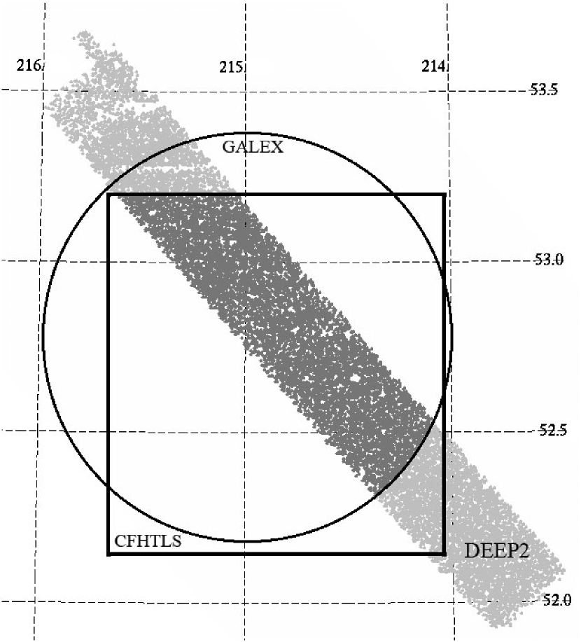
GALEX (Martin et al., 2005; Morrissey et al., 2007) imaged the central portion of the EGS with a single $1.2\arcdeg$ diameter pointing (Figure 1). The exposure time was 237 ks in the near-UV (NUV) and 120 ks in the far-UV (FUV) band, which makes it the deepest GALEX single pointing to date. Data are taken from public release GR3. While GALEX observes in FUV and NUV simultaneously, 1/2 of the FUV exposure time was lost due to anomaly with the FUV detector (Morrissey et al., 2007). The GALEX pipeline produces catalogs using SExtractor (Bertin & Arnouts, 1996) aperture photometry. While adequate for more shallow, resolved images, such photometry suffers from severe blending and source confusion in the deep EGS images (GALEX resolution is $4-5^{\prime\prime}$, while astrometry is good to $0\farcs 5$, Morrissey et al. 2007). To remedy this problem we perform PSF source extraction, which is less sensitive to blending (Zamojski et al., 2007). We use the custom-built PSF extraction software EM Photometry, developed by D. Aymeric, A. Llebaria and S. Arnouts, which uses the expectation-maximisation (EM) algorithm of Guillaume et al. (2006). EM Photometry extracts GALEX fluxes based on optical prior coordinates. While successfully dealing with blending, the resulting fluxes for a given set of objects will to some extent depend on the depth (i.e., the number of objects) in the prior catalog, with photometric bias being especially pronounced for intrinsically fainter objects. In particular, having too many faint optical priors (fainter than the equivalent GALEX limit in the absence of blending) will result in the splitting of the UV flux of one object among multiple sources, most of which are not actually detectable in GALEX images. We minimize this bias by using the list of optical priors based on $u$-band (band closest to NUV) photometry from the CFHT Legacy Survey (§2.3) and choosing a $u$ limit of 25.5, at which the majority of optical objects still have real counterparts in the NUV image. After extracting the NUV fluxes using the $u$-band prior catalog, we find that genuine detections mostly have NUV$<26.5$, which we adopt as a cut for the NUV catalog, and which roughly corresponds to 3$\sigma$ limit. As a cross-check we also perform source detection and PSF extraction using DAOPHOT (Stetson, 1987), i.e., without positional constraints on source detections. Comparing the results from DAOPHOT and EM Photometry for relatively isolated sources, we find a good agreement for NUV$<24$, and a gradually increasing difference at fainter magnitudes, up to 0.21 mag at the catalog limit (DAOPHOT photometry being brighter). The difference can likely be attributed to unresolved detections in DAOPHOT, and it also represents the upper limit on the above-discussed bias introduced by forcing prior extractions. With an NUV catalog in hand, we repeat the procedure to obtain FUV photometry, now using NUV$=26.5$ to set the cut on the prior catalog and adopting a FUV$=26.5$ cut for the final FUV catalog (roughly a 3$\sigma$ limit). We estimate the bias at the faint end to be below 0.13 mag. The FUV and NUV catalogs are matched to the CFHTLS catalog by construction, which is in turn matched to DEEP2 positions (§2.3). Of CFHTLS sources matched to the full DEEP2 redshift catalog, 22% have fluxes in FUV caalog and 59% in NUV catalog. RMS calibration errors of 0.052 and 0.026 mag are adopted for FUV and NUV respectively (Morrissey et al., 2007).

2.3. CFHT Legacy Survey optical photometry

The EGS represents one of the four deep fields targeted by the CFHT Legacy Survey (CFHTLS). The central region of the EGS is observed with the MegaPrime/MegaCam imager/detector in a single pointing covering a $1\arcdeg\times 1\arcdeg$ field of view (Figure 1) in five optical bands ($u^{*}g^{\prime}r^{\prime}i^{\prime}z^{\prime}$). The limiting magnitudes corresponding to 80% completeness are 27.2, 27.5, 27.2, 27.0, 26.0, respectively. We use band-merged catalogs (publicly available version 2008A) based on $i$-band detections, with aperture photometry measured from $i$-band derived apertures. Matching to the DEEP2 redshift catalog is performed using a $0\farcs 3$ search radius. Astrometric zero points coincide to within $0\farcs 02$, and the 1-D coordinate scatter between the two catalogs is $0\farcs 08$, i.e., both catalogs have very accurate astrometry. There are no multiple matching candidates. Of 9923 DEEP2 objects (from the full redshift catalog not restricted to good quality redshifts) that lie within CFHTLS coverage, 9056 (91%) are matched. Based on the scatter of the comparison of the bright end with SDSS, we adopt RMS calibration errors of (0.04,0.025,0.025,0.025,0.025,0.035) mag for ($u^{*}g^{\prime}r^{\prime}i^{\prime}z^{\prime}$).

2.4. MMT $u$-band photometry

In addition to $u^{*}$-band data from CFHTLS, we also use $u^{\prime}$-band photometry obtained with MegaCam (McLeod et al., 2006) on the MMT. These data extend across nearly the entire length of the EGS, with 24 overlapping fields each covering $0.4\arcdeg\times 0.4\arcdeg$. The $5\sigma$ limiting magnitude varies between 26.3 and 27.0. Matching to the DEEP2 redshift catalog was performed using a $0\farcs 4$ search radius after applying a $0\farcs 18$ offset in declination to bring the coordinate system of MMT data (based on USNO-B1) into agreement with the SDSS system used in DEEP2. The 1-D coordinate scatter between the two catalogs is $0\farcs 12$. Of 15283 DEEP2 objects (from the full redshift catalog) within MMT coverage, 10965 have a match (72%), with a handful of multiple match candidates, in which case the object with brighter $u^{\prime}$ is selected.

Since we have $u$-band photometry from CFHTLS as well, we can compared them. The scatter between the MMT and CFHTLS $u$-band magnitudes does not increase with DEEP2 matching separation, indicating that the matches are real throughout the search radius. However, there is a 0.08 mag overall offset between two magnitudes in the sense that CFHTLS $u$ is fainter than MMT $u$. At the bright end we can compare these magnitudes to SDSS. MMT $u$ matches SDSS very well, while CFHTLS $u$ is again fainter, but by 0.05 mag (both MMT and CFHTLS photometry was first transformed to SDSS system). The offsets between MMT and CFHTLS $u$ do not show an obvious color dependence. We correct these offsets in the SED fitting. We adopt a calibration RMS error of 0.04 mag for MMT photometry.

2.5. Palomar $K$-band photometry

The reddest photometry band that we use in the SED fitting comes from the Palomar $K$-band survey of DEEP2 (Bundy et al., 2006, 2008). Including redder bands (such as IRAC 3.6 and 4.5 $\mu$m) would not place additional constraints on SFRs, which are the main focus of this paper. The EGS is almost fully covered with thirty-five $8\farcm 6\times 8\farcm 6$ WIRC frames, down to a 21.7–22.5 mag limit at 80% completeness. We use MAG_AUTO fluxes from the Bundy et al. (2006) SExtractor catalog, and their $1\farcs 1$ matching to DEEP2. Of 16087 DEEP2 objects from the full redshift catalog, most of which are within $K$ survey coverage, 10398 (65%) have a match.

2.6. MIPS Spitzer 24 $\mu$m photometry

In addition to UV through near-IR data that are used for the SED fitting, we use 24 $\mu$m observations to estimate IR luminosities. The 24 $\mu$m data were obtained with MIPS on Spitzer as part of the FIDEL survey. FIDEL observed EGS and ECDF-S fields with MIPS at 24 and 70 $\mu$m to depths of 30 $\mu$Jy and 3 mJy, respectively. These depths approach those of GOODS yet cover a larger area. In EGS, these data are five times deeper than the previous data described in Davis et al. (2007) (which are co-added to FIDEL data). We extract PSF fluxes from 24 $\mu$m images using DAOPHOT (MIPS has $6^{\prime\prime}$ resolution at 24 $\mu$m; Rieke et al. 2004). We then match 24 $\mu$m sources having S/N$>3$ (corresponding to 10-16 $\mu$Jy) to the CFH12K photometry catalog (Coil et al., 2004) using a $1\farcs 5$ matching circle. This search radius is appropriate for bright 24 $\mu$m sources, which have a 1-D astrometry precision of $0\farcs 5$. However, fainter sources have poorer astrometry, so we subject sources that initially had no match (39% of total) to a larger $3^{\prime\prime}$ radius search, recovering some 60% of them. In cases of multiple optical candidates (4% of cases), we pick the one that has the $I$-band to 24 $\mu$m flux ratio that is at least two times more likely than that of other candidates, where the probability is based on the flux ratio distribution of unique matches. This allows us to resolve 30% of multiple matches. We consider the remaining multiple matches to be a blend of more than one optical source and exclude them from the catalog of matched sources and from further analysis. Altogether, an optical match is determined for 74% of 24 $\mu$m sources within the optical coverage. The unmatched 24 $\mu$m sources are either blends or are presumably fainter than the $R=24.5$ limit of CFH12K photometry catalog. Similar detection rates (for similar $R$ limits) were found in CDF-S by Pérez-González et al. (2005) and by Le Floc’h et al. (2005), 70% and 60%, respectively. In the opposite direction, of DEEP2 objects from the full redshift catalog, 6581 (41%) are detected at 24 $\mu$m. We decide to match 24 $\mu$m data directly to optical instead of using IRAC photometry (Barmby et al., 2008) as an intermediate step, because IRAC coverage of EGS is not as extensive. As a test, for areas with IRAC coverage we run matching via IRAC and find that in 98% of cases we obtain the same optical match as with direct 24 $\mu$m to optical matching.

2.7. Other data and data products

In addition to redshifts, DEEP2 spectra provide emission line fluxes which we use to select narrow-line AGNs. Derivation of fluxes is described in Weiner et al. (2007). We also use Chandra X-ray detections from AEGIS-X DR2 to select X-ray AGN. Details of the X-ray data, catalog construction and matching to optical sources are given in Laird et al. (2009).

3. UV/optical SFRs from SED fitting

The sample used in SED fitting consists of DEEP2 galaxies with secure redshifts and spectra classified as galaxies. A small number of galaxies fitting an AGN template (broad-line AGNs, QSOs) are excluded since their continua will be affected by the light from the active nucleus, and therefore cannot be fitted with our models. In terms of area, our sample lies in the overlap of CFHTLS and GALEX regions (dark gray region in Figure 1), which contains 5878 DEEP2 galaxies. Other data cover this region fully, so their footprints are not relevant. Using a technique similar to that of Blanton (2006) we first estimate the area of the full DEEP2 EGS (light and dark gray region in Figure 1). Our sample contains 53% of the total number of sources in full area, from which we arrive at an estimate of 0.31 sq. deg. for the overlap area (dark gray region in Figure 1 . We remind the reader that detections are not required in all bands as long as the object comes from the overlap area, so our optical sample used in SED fitting remains only $R$-band selected.

We estimate galaxy parameters such as the star formation rate, dust attenuation, stellar mass, age, rest-frame colors and magnitudes, using the stellar population synthesis models of Bruzual & Charlot (2003). The methodology is basically identical to that used in Salim et al. (2007, S07), and we refer the reader to that paper for details of stellar population and attenuation models. Model libraries are built by considering a wide range of star formation histories (exponentially declining continuous SF with random stochastic bursts superimposed), with a range of metallicities (exact ranges are given in S07). Each model is dust-attenuated to some degree according to a two-component prescription of Charlot & Fall (2000). This model assumes that young populations ($<10$ Myr) lie within dense birth clouds and experience total optical depth of $\tau_{V}$. When these clouds disperse, the remaining attenuation is only due to the general ISM, having optical depth of $\mu\tau_{V}$, where $\mu$ is typically $\sim 0.3$. In both cases the extinction law of a single population is $\propto\lambda^{-0.7}$. In our models, we allow for a range of $tau_{V}$ and $\mu$ values as described in S07. A feature in the SED that has the greatest weight in constraining the dust attenuation is the UV slope, which is steeper (the UV color is redder) when dust attenuation is higher (Calzetti et al., 1994). However, there is a significant scatter between the UV slope and the dust attenuation due to the differences in the SF history (Kong et al., 2004), which in our model is constrained by the inclusion of optical data. Finally, we include reddening due to the intergalactic medium, according to Madau et al. (1996). SFRs and stellar masses are determined assuming a Chabrier IMF.

The only difference in model libraries with respect to S07 is that we now construct them in $0\leq z_{\rm lib}\leq 1.6$ range, at 0.1 intervals in $z_{\rm lib}$, whereas in S07 libraries extended out to $z_{\rm lib}=0.25$ at 0.05 intervals. While library redshift resolution is finite, note that we use exact galaxy redshifts to scale mass and SFR from normalized model quantities to full absolute values. We test the effects of library redshift coarseness on the derivation of SFR and mass. On average, redshift and $z_{\rm lib}$ differ by 1/4. We produced a test run where we increase this difference to 3/4 by assigning the next or the preceding library (e.g., galaxy at $z=0.97$ is fitted with $z_{\rm lib}=1.1$ models instead of $z_{\rm lib}=1.0$). As expected, the average values of SFR and stellar mass do not change, but the average absolute difference is 0.13 dex for SFR and 0.09 dex for stellar mass. From this we can extrapolate that when redshift and $z_{\rm lib}$ differ by 1/4 this deviation will be 0.04 and 0.03 dex, respectively. In our analysis this will be reflected as the small addition to the random errors. Finally, since only models with formation age shorter than the age of the universe at $z_{\rm lib}$ are allowed, the number of model galaxies decreases from $10^{5}$ at $z_{\rm lib}=0$ to $3\times 10^{4}$ at $z_{\rm lib}=1.6$. Even at the high-redshift end the number of models is sufficiently large not to introduce biases in the derived parameters (Salim et al., 2007).

Our SED fitting involves up to 9 flux points (FUV, NUV, $u^{\prime}_{\rm MMT}$, ($u^{*}g^{\prime}r^{\prime}i^{\prime}z^{\prime})_{\rm CFHTLS}$, $K$), their photometric errors, and the redshift. Photometry for various bands has been derived in a heterogeneous manner, but it should reflect the total fluxes in most bands. This will have a negligible effect on the results. The SED fitting has one degree of freedom (scaling between the observed and the model flux zero points). For each galaxy the observed flux points are compared to model flux points, and the goodness of the fit ($\chi^{2}$) determines the probability weight for the given model, and thus of the associated model parameters in the final probability distribution function (PDF) of each parameter (such as the SFR, stellar mass, etc.). We then use the average of the probability distribution as our nominal estimate of a galaxy parameter and consider the width of the probability distribution function as an estimate of parameter error and its confidence range. In cases where no detection is present in a given band, that band does not contribute to $\chi^{2}$. The Bayesian SED fitting performed here has many advantages with respect to more traditional maximum likelihood method. The parameter PDFs allow us to determine how well a given parameter can be determined taking into account not only the observational errors, but also the degeneracies among the models. For example, suppose that the dust attenuation and the metallicity were completely degenerate, i.e., that various combinations of the two produce identical SEDs. While the maximum likelihood will pick one (basically arbitrary) SED and its parameters as the best fitting, the Bayesian fitting will produce a wide flat PDF suggesting that many different values are equally probable. Similarly, the lack of observational constraints will also be reflected in the increased width of PDFs of those parameters that rely on these observations. While all flux points contribute to all galaxy parameters, it is to be expected that the UV fluxes will be more critical in obtaining current SFRs and dust extinctions, while flux points red-ward of 4000Å will contribute more to the determination of the stellar mass. Also, we note that despite the fact that our input (observed SED) contains limited information content, one could in principle derive an unlimited number of galaxy parameters, since the PDF of each parameter will correctly marginalize over observational and model uncertainties. Most of these parameters will, of course, not be independent, which one can again establish using (multidimensional) PDFs. Reader is referred to S07 for further details about the SED fitting procedure. Walcher et al. (2008), who use very similar model libraries and the fitting technique, also provide extensive discussion on the method and its robustness (their §2). In § 4 we will discuss in more detail the errors in the SFR.

Before performing the SED fitting, we first examined color-color diagrams where we plot observed colors in some redshift interval together with model colors corresponding to that redshift. We were prompted to perform these tests after learning that there could be a discrepancy between the observed and Bruzual & Charlot (2003) colors in the VVDS sample, in the sense that models were underestimating the flux in the 3300-4000 Å range (Walcher et al., 2008). By visually comparing the locus of observed and model colors for various combinations of colors and redshift bins, we were mostly able to confirm this effect. We find the level of discrepancy (up to 0.2 mag) to be similar for both blue and red galaxies, which makes it unlikely to be the result of contamination from [OII]$\lambda$3727 emission line (emission lines are not included in Bruzual & Charlot 2003 modeling) but, rather caused by differences in the continuum. Walcher et al. (2008) use an updated version of Bruzual & Charlot (2003) models (which include new prescriptions for TP-AGB stars) and still encounter the discrepancy. However, both the original Bruzual & Charlot (2003) models used here and the updated version used by Walcher et al. (2008) are based on same stellar libraries which have a transition from empirical STELIB spectra to synthetic BaSeL spectra at 3200 Å. It is beyond the scope of this work to try to understand the origin of this problem. Since at a given redshift this discrepancy would affect only one of our flux points, we decide to exclude that flux point from the SED fitting, i.e., we exclude $g$ at $0.3\leq z_{\rm lib}\leq 0.5$, $r$ at $0.7\leq z_{\rm lib}\leq 0.9$, $i$ at $1.0\leq z_{\rm lib}\leq 1.3$, and $z$ at $z_{\rm lib}=1.4$.

We require a minimum of three flux points for the SED fitting, though most galaxies have many more. In 336 cases this criterion is not met (mostly because CFHTLS magnitudes are not measured in spite of the fact that the object is listed), and we exclude these objects from further analysis. Additionally, we eliminate 197 objects with poor SED fits (i.e., high $\chi^{2}$) whose galaxy parameters are unreliable. In S07 we discuss galaxies with bad SED fits and conclude that they mostly result from bad data rather than the limited parameter space of the models. Thus we arrive at the final optical sample of 5345 objects for which we obtain galaxy parameters from the SED fitting.

Figure 2.— Errors in the current (upper panel) and age-averaged (lower panel) star formation rates, both corrected for dust attenuation and plotted against the rest-frame color. Errors are estimated from the width of the probability distribution function and take into account measurement and model uncertainties, such as the uncertainty in the dust correction.

Two parameters derived from the UV/optical SED fitting will feature most prominently in this work: the “current” SFR (i.e., the SFR averaged over the last $10^{8}$ yr, the shortest timescale that can be reliably probed with stellar continuum) and the “age-averaged” SFR (i.e., the SFR averaged over the dominant population age, which depends on a galaxy and typically ranges between 1-3 Gyr). Both will be discussed in more detail later. Here we wish to assess the typical errors associated with these parameters. Both SFRs are dust-corrected and their probability distribution functions will automatically reflect various sources of uncertainty. In the case of the current SFR the error will be dominated by the uncertainties in the dust correction, which we confirm by finding a strong correlation between SFR error and dust correction error. In Figure 2 (upper panel) we show the error in current SFR ($t_{\rm SF}=10^{8}$ yr) as a function of rest-frame ${\rm NUV}-R$ color, which we will use to select actively star-forming (blue) and quiescent (red) galaxies. The error equals 1/4 of the 95% confidence range of a PDF, which in the case of a Gaussian distribution would correspond to a standard deviation ($1\sigma$). The majority of galaxies have errors below 0.2 dex (60%). As expected, the errors increase as one moves towards redder, less actively star-forming galaxies. Some galaxies, regardless of color, have an error in excess of a factor of 3 (0.5 dex). We find that these galaxies are very faint in the UV, with rest-frame FUV magnitudes fainter than 24.5. Figure 2 (lower panel) shows errors in age-averaged SFR. Unlike the current SFR which is mostly constrained by rest-frame UV, the age-averaged SFR is determined by optical light of stars having ages 1-3 Gyr. It is also typically less than 0.2 dex, but it is on average higher for blue galaxies where the optical light is fainter. Unlike the current SFR, here the errors stay below 0.5 dex, owing to the lack of very faint optical sources (the sample being $R$-band selected). While the stellar mass doesn’t figure prominently by itself in this work, let us mention that the typical stellar mass errors are below 0.1 dex.

Figure 3.— The effect of H$\alpha$ contamination on the SFRs derived from the SED fitting. In the displayed redshift range the H$\alpha$ passes through $z$ filter (its relative contribution to $z$ is shown as a solid curve with arbitrary amplitude) and could thus affect the SED fitting. Shown is the difference in age-averaged SFRs (SFR with subscript ’a’) when the $z$ band is excluded from the fitting, compared to nominal fitting. Mean residuals (solid line slightly above the $y=0$ line) are below 0.02 dex and are not correlated with the expected H$\alpha$ contribution. We plot only blue, star-forming galaxies for which the contribution of H$\alpha$ should be the largest.

Galaxy SED models used in this work come from stellar population synthesis alone, without the inclusion of gas emission lines. This could potentially lead to systematic effects in the parameters derived from the SED fitting, since the emission lines could “contaminate” the broad-band fluxes used in the fitting. Typically, the most luminous emission line in our sample is H$\alpha$, followed by [OII]$\lambda$3727. H$\alpha$ becomes redshifted beyond the reddest optical band ($z$ band) at redshifts above 0.4, so it does not affect most of the galaxies in our sample. For those at lower redshift we estimate the effect of H$\alpha$ contribution by running the SED fitting without the $z$ band and comparing the resulting SFRs to those from the nominal fitting. The residuals of age-averaged SFRs are shown against the redshift in Figure 3 for blue (mostly star-forming) galaxies. We present age-averaged SFRs since they should be more affected by the $z$-band flux than the current SFRs. Typical average residuals are below 0.02 dex, and there is no obvious correlation with the expected relative contribution of H$\alpha$ to $z$-band (solid curve, shown with arbitrary amplitude). Residuals tend to be positive, which actually corresponds to SFRs from the fit without the $z$ band being larger than the nominal ones, the opposite from what is expected if H$\alpha$ raises the $z$-band flux. As for [OII] line, one cannot evaluate its potential effect on broad-band fluxes because of the unrelated issues with models in the 3300-4000 Å range (discussed previously in this section). Since we already exclude from SED fitting the bands that sample this wavelength range, any effects of [OII] will be removed from our nominal results.

4. Infrared and optical properties of 24 $\mu$m sample

Figure 4.— Detection fraction of MIPS 24 $\mu$m observations in bins of redshift and apparent magnitude. Gray pixels represent the detection fraction, with black being 100% and white being zero, except in the upper right corner where there are no objects.

Figure 5.— Rest-frame color distribution of the sample. Bold histogram shows the distribution of our optical ($R<24.1$) sample (for which the SED fitting is performed), and the thin histogram shows the distribution of sample sources which are detected at 24 $\mu$m. The dashed line is the ratio of the two histograms, i.e., 24 $\mu$m detection fraction. The 24 $\mu$m detection fraction peaks at the red end of the blue sequence and in the “green valley”. In this and subsequent figures, superscript zero in NUV$-R$ designates rest-frame (note that NUV$-R$ is not dust corrected).

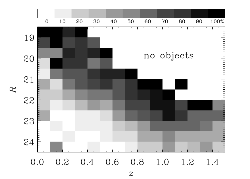
Out of 5345 objects in the optical sample, we have 24 $\mu$m detections for 2430 (45%). The 24 $\mu$m imaging covers 99.5% of the area of the optical sample, with exposure times varying across the field from $\sim 0$ to 19 ks (average exposure is 10 ks). The optical source detection efficiency grows linearly with the logarithm of the exposure time; it is 26% at 1 ks, and 56% at 19 ks. In Figure 4 we plot the 24 $\mu$m detection efficiency as a function of redshift and apparent $R$ magnitude. The gray scale is proportional to the detection fraction, with black representing 100% and white being zero, except at bright magnitudes and high redshifts where there are no objects. At each redshift the detection fraction increases with optical brightness, but for a given $R$ magnitude the efficiency increases with redshift, which is the consequence of the detection efficiency rising with absolute magnitude. In Figure 5 we plot the distribution of rest-frame ${\rm NUV}-R$ colors determined from the SED fitting. The optical sample (bold histogram) is dominated by galaxies lying in the blue sequence (${}^{0}({\rm NUV}-R)<3.5$). The peak of the red sequence (${}^{0}({\rm NUV}-R)>4.5$) is less obvious because the $R$-band selection eliminates fainter red galaxies at higher redshifts. The thin-line histogram shows galaxies with 24 $\mu$m detection. Again, most detections are of blue galaxies. The ratio of the two histograms represents the 24 $\mu$m detection fraction and is plotted as the dashed curve with a corresponding axis on the right-hand side. The 24 $\mu$m detection efficiency strongly peaks at intermediate colors, including the so called “green valley” ($3.5<^{0}({\rm NUV}-R)<4.5$), where it reaches $>80\%$. A similar result was recently obtained by Cowie & Barger (2008).

Figure 6.— Relation between the rest-frame UV-to-optical color and the specific SFR of the part of the optical sample detected at 24 $\mu$m. The two quantities are roughly equivalent, except that the specific SFR, derived in UV/optical SED fitting, is dust-corrected. Also, SFR is averaged over $10^{8}$ yr, which we call “current” SFR (subscript ’c’). In cases of moderate dust UV-to-optical color correlates with the SF history of a galaxy (the trend of the majority of galaxies in this sample). Galaxies that scatter away from that relation are dusty starbursts (objects above the dashed line). Note that many genuine red sequence (and not just reddened), i.e. quiescent, galaxies are still detected at 24 $\mu$m. The classification of colors into blue, green, and red, and the SF histories into active star-forming, transitional and quiescent is based on local ($z<0.2$) studies that employ photometry and spectroscopy to distinguish between these categories (Wyder et al., 2007; Salim et al., 2007).

Motivation for the above division into blue and red sequence galaxies comes from a marked bimodality in optical colors of local ($z<0.2$) galaxies (Strateva et al., 2001), where blue sequence galaxies have active star formation, while red have generally ceased forming stars. The introduction of UV-to-optical colors by GALEX led to a recognition of a region in between the blue and the red sequences that was not prominent in optical colors (Wyder et al., 2007). Galaxies that occupy this region, the green valley, acquire intermediate colors either because they have an intermediate SF history (transitional galaxies), or because their colors have been reddened by dust and would otherwise be blue (dusty starbursts) (Martin et al., 2007; Salim et al., 2007). One can distinguish between the two by plotting the specific SFR (SFR/$M_{*}$) against the color. This is shown in Figure 6, where the rest-frame color, dust-corrected SFR and the stellar mass come from our UV/optical SED fitting, and the SFR is what we call current, i.e., averaged over $10^{8}$ yr. If dust reddening is moderate, there should be a correlation between the specific SFR (basically a ratio of recent to past SF) and the rest-frame UV-to-optical color (Salim et al., 2005). One can see that this is the case for the majority of galaxies, especially in blue and red regions. However, if a galaxy has dusty star formation, it will have redder colors for a given specific SFR (because the SFR is corrected for effects of dust, while color is not). Such galaxies scatter above the main trend in Figure 6 (galaxies above the dashed line). In terms of colors, dusty starbursts are present in the blue sequence and the green valley, with the relative number of dusty to non-dusty systems peaking in the green valley. Here we note that even after accounting for dust attenuation there still exist 24 $\mu$m detections among fairly quiescent galaxies ($\log({\rm SFR}/M_{*})<-11$). The source of their mid-IR emission will be discussed in §6.

Figure 7.— Comparison of IR luminosities obtained with various IR templates and the 24 $\mu$m flux point. Comparison is against ${L_{\rm IR}}$ obtained with Dale & Helou (2002) templates (DH02). The difference is relatively small with respect to Chary & Elbaz (2001) templates (CE01), but more significant with respect to Rieke et al. (2009) templates (R09), especially at higher luminosities. We use IR luminosities based on Dale & Helou (2002) in the rest of the paper.

To infer the total infrared luminosity, ${L_{\rm IR}}$(8–1000$\mu$m), we fit 24 $\mu$m flux densities and redshifts to infrared SED templates of Dale & Helou (2002). These templates were normalized to follow the local IRAS-calibrated far-IR color vs. luminosity relation of Marcillac et al. (2006). The assumption is that for most galaxies in our sample the mid-IR flux is representative of the total IR luminosity, and that one can use the luminosity-dependent SED models to constrain it. This is certainly an oversimplification. The rest-frame wavelength range probed by our 24$\mu$m observations (10–18$\mu$m) contains many PAH lines whose relation to the mid-IR continuum and to the total IR luminosity may vary significantly compared to the fixed ratios assumed in the templates (Smith et al., 2007). Also, translating mid-IR luminosities to total ones introduces potentially large uncertainties in the $K$ correction. However, the use of total vs. mid-IR continuum luminosities is not critical in this work, and, as we will show in §7.3, the results do not change if we use monochromatic mid-IR luminosity instead. The use of total IR luminosity is motivated by the commonality with which this measure is interpreted as a star formation rate, especially in high-redshift studies. Once we obtain the interpolated IR template, we calculate the total infrared luminosity according to the relation of Sanders & Mirabel (1996) (directly integrating the SED produces very similar results, and Sanders & Mirabel definition is used as a convention). In addition to ${L_{\rm IR}}$ derived from Dale & Helou (2002) templates, we additionally calculate ${L_{\rm IR}}$ based on luminosity-dependent templates of Chary & Elbaz (2001) and recent templates of Rieke et al. (2009). The comparison of the two with respect to ${L_{\rm IR}}$ from Dale & Helou (2002) is shown in Figure 7. For our sample the IR luminosities from Chary & Elbaz (2001) and Dale & Helou (2002) stay within 0.2 dex of one another (average difference is -0.03 dex and the standard deviation of the ratio is 0.09 dex). At $\log{L_{\rm IR}}\rm{(DH02)}>11$ the scatter in the ratio is very small (0.02 dex), and the difference is almost constantly around -0.06 dex (Dale & Helou (2002) estimate being higher). Differences with respect to Rieke et al. (2009) IR luminosities are much higher, especially for LIRGs and ULIRGs ($\log{L_{\rm IR}}\rm{(DH02)}>11$). Rieke et al. (2009) estimates get increasingly discrepant as the luminosity increases (up to an order of magnitude), to the extent that 16% of what are classified as LIRGs according to Dale & Helou (2002) become ULIRGs with Rieke et al. (2009) templates, while the number of ULIRGs changes from 21 to 156. Using Rieke et al. (2009) templates could possibly affect some of the results in our work, but also those of many other studies. On the other hand, the differences between the other two templates are smaller (see also Pérez-González et al. 2008), and we adopt IR luminosities based on Dale & Helou (2002) templates as our nominal values. All of these templates are based on local, star-forming galaxies, so they may not be entirely appropriate for high redshift galaxies such as those in our sample, or to more quiescent galaxies. In our analysis we will therefore use caution when interpreting the IR luminosities.

Figure 8.— Infrared luminosity ${L_{\rm IR}}$, derived from 24 $\mu$m flux, as a function of redshift. Two dashed lines define LIRGs ($11<\log{L_{\rm IR}}<12$), and ULIRGs ($\log{L_{\rm IR}}>12$). Normal star forming galaxies ($\log{L_{\rm IR}}\sim 10$) are detected to $z\sim 0.7$. There are very few ULIRGs in our sample.

In Figure 8 ${L_{\rm IR}}$ is shown as a function of redshift. Two dashed lines show regions that define LIRGs and ULIRGs. LIRGs start to dominate raw counts at $z\sim 0.8$ and we remain sensitive to LIRG luminosities out to the upper redshift limit. We are also sensitive to normal star forming galaxies (${L_{\rm IR}}\sim 10^{10}L_{\odot}$) to $z\sim 0.7$. The number of ULIRGs is small even at the highest redshifts. This is similar to the luminosity distribution presented in Le Floc’h et al. (2005) for CDF-S. Since we study only 24 $\mu$m detections with available spectroscopic redshifts, we check if the redshift selection introduces any biases at the high-luminosity end of ${L_{\rm IR}}$. For this purpose we consult a catalog of photometric redshifts based on CFHTLS photometry (Ilbert et al., 2006), and match it to optical counterparts of 24 $\mu$m sources. We then compute ${L_{\rm IR}}$ based on photometric redshift. For ${L_{\rm IR}}>10^{9.4}L_{\odot}$ the distribution of ${L_{\rm IR}}$ of the photometric redshift sample matches the shape of the distribution of ${L_{\rm IR}}$ in our spectroscopic redshift sample, implying no bias of the latter at high IR luminosities.

5. Infrared luminosity and UV/optical SFR in blue sequence galaxies

We now have on one hand dust-corrected SFRs constrained from UV/optical SED fitting, and on the other hand infrared luminosities from 24 $\mu$m flux. We will often refer to dust-corrected UV/optical SFRs as SED SFRs, or just SFRs. We emphasize that SED fitting allows us to construct SFRs on various timescales, i.e., SFR averaged over some time interval. They are chosen to be $t_{\rm SF}=10^{7}$, $10^{8}$, $10^{9}$ and $2\times 10^{9}$ yr (averaging interval $t_{\rm SF}$ ends with the epoch of the observation, i.e., it is not centered on it). In addition to these fixed timescales, we also determine SFR averaged over the age of the galaxy, which is calculated as the total stellar mass (current mass plus the recycled mass as estimated in our models) divided by the time since galaxy formation (from models). Because in our models the galaxy formation ages have a uniform distribution, i.e., they are not restricted to some high-redshift galaxy formation epoch, the derived formation age will be largely driven by the age of the dominant population in terms of light production (for example, blue galaxies will be assigned young “formation” ages regardless of their “real” age). We verify that there is a very tight correlation between the derived “formation” age and the light-weighted age. Therefore, what is actually measured by age-averaged SFR is the average SFR over the age of the dominant population, which for blue-sequence galaxies in our sample varies between 0.1 and 3 Gyr. Errors in UV/optical SFRs were discussed in §3 for the full optical sample and those conclusions are applicable here for the subset detected at 24 $\mu$m.

Since the IR luminosity is usually considered in the context of (current) star formation rate, we begin our analysis using the concept of star formation rate, but extending it to include SFRs averaged over longer time periods. The temporal aspect is not essential here. The timescales used in averaging the SFR simply correspond to the light emitted today by stellar populations of different ages. Therefore, what constrains the SFRs averaged over progressively longer timescales is the rest-frame luminosity at increasingly redder wavelengths. We will return to this relation between SFR and luminosity later.

Figure 9.— Comparison of infrared luminosities and dust-corrected UV/optical star formation rates for all galaxies. Throughout the paper the SFRs are given in $M_{\odot}{\rm yr}^{-1}$ and for Chabrier IMF. UV/optical SFR is averaged over $10^{8}$ yr (“current” SFR, subscript ’c’), the characteristic UV timescale. Numbers in lower right corner show the dispersion ($\sigma$) and the mean offset ($\Delta$) (in dex) with respect to the 1:1 correspondence between the SFR and infrared luminosity (solid line) that assumes the Kennicutt (1998) conversion (converted to Chabrier IMF). The Kennicutt conversion is derived for dusty star-forming galaxies with constant SFRs over $10^{7}$–$10^{8}$ yr.

The timescale corresponding to lifetime of stars producing the majority of non-ionizing UV radiation is $\lesssim 10^{8}$ yr (Kennicutt, 1998). Since young stars are typically assumed to dominate the dust heating at mid-IR (§1), we begin by comparing the infrared luminosity with SED SFR averaged over $t_{\rm SF}=10^{8}$ yr, which can be regarded a “current” SFR. In Figure 9 we plot all 2430 galaxies from our optical sample detected at 24 $\mu$m. The line represents the 1:1 correspondence between the SFR and the infrared luminosity assuming the Kennicutt conversion (converted to Chabrier IMF by applying a factor of 1.58, S07). It is important to recall that the Kennicutt conversion applies to optically thick dusty starbursts with constant SF histories over $10^{7}$–$10^{8}$ yr and solar metallicities. The conversion factor is not empirical, but is derived from population synthesis models. While it is not strictly appropriate to use this conversion for other types of galaxies (less dusty or less active), such practice is often encountered. This can be somewhat justified because, as shown in modeling of Inoue (2002), the fortuitous cancellation of smaller dust opacity and the increased IR cirrus causes the Kennicutt conversion to also hold for less bursty (more normal) SF galaxies. In any case, conclusions in our work are independent of the validity of conversions of IR luminosity to SFR, and instead we deal with IR luminosities directly. In Figure 9 one sees a good overall agreement between the IR luminosity and the UV/optical SFR. The points on average lie 0.02 dex from the 1:1 line. The standard deviation in the logarithm of ${L_{\rm IR}}$ to SFR ratio, i.e., the scatter around the 1:1 line, is 0.49 dex (a factor of three). It is the scatter that we will use as an indicator of the level of agreement between the IR luminosity and the SED-derived UV/optical SFR.

There are a number of potential causes for the level of scatter seen in Figure 9. First, there are measurement errors. On average, the error in “current” SFR is 0.19 dex. The average error in 24 $\mu$m flux measurement is 6% (0.02 dex), which is negligible in comparison. We expect some error from the extrapolation of the observed 24 $\mu$m (rest frame 10–18 $\mu$m) luminosity to total IR luminosity (e.g, Le Floc’h et al. 2005 claim a factor of three error). As discussed, the two frequently used sets of IR SED templates already produce a scatter of 0.1 dex in their estimate of ${L_{\rm IR}}$. Another source of scatter could be from from the inclusion of all galaxies in our sample, including many red galaxies with older stellar populations and not much current star formation. In order to compare UV/optical SFR and ${L_{\rm IR}}$ with an assumption that IR arises from star formation, one needs to limit the sample to actively star forming galaxies. Following discussion in §4 it would be appropriate to base such selection on a dust-corrected quantity such as the specific SFR. However, it is more intuitive to use rest-frame color instead. Taking blue galaxies (${}^{0}({\rm NUV}-R)<3.5$) will select most actively star-forming galaxies (including a large number of dusty starbursts), while not allowing galaxies with more quiescent SF histories (Figure 6). In Figure 10, we now compare ${L_{\rm IR}}$ and SED SFR of blue galaxies alone. The SFR averaging timescale is still $10^{8}$ yr. The scatter in ${L_{\rm IR}}$ to SFR ratio is 0.42 dex, or 16% smaller than in the full sample. The scatter was reduced by the removal of red galaxies. This reduction cannot be attributed to slightly smaller SED SFR errors: 0.17 dex for blue galaxies vs. 0.19 dex for the full sample.

Figure 10.— Comparison of infrared luminosities and dust-corrected UV/optical star formation rates for blue-sequence galaxies. Timescale for SF is still $10^{8}$ yr, and the Kennicutt (1998) conversion (derived for dusty star-forming galaxies with constant SFRs over $10^{7}$–$10^{8}$ yr) is shown as the solid line. Removal of red galaxies reduces the scatter in correlation. Numbers have the same meaning as in Fig. 9

Figure 11.— Comparison of infrared luminosities and dust-corrected UV/optical star formation rates for blue-sequence galaxies, where SFR is now averaged over the galaxy age (i.e., the age of the dominant population, 0.1–3 Gyr old, subscript ’a’). The correlation between ${L_{\rm IR}}$ and SFR is better (the scatter is smaller) than in Figure 10, where SFR was averaged over $10^{8}$ yr. The error in the SFR determination is similar here as it is for SFR averaged over $10^{8}$ yr ($\sim 0.2$ dex), and does not dominate the scatter with respect to ${L_{\rm IR}}$. There is a departure with respect to Kennicutt (1998) conversion which is derived for dusty star-forming galaxies with constant SFRs over $10^{7}$–$10^{8}$ yr, because most galaxies have declining SF histories so the SFRs averaged over longer timescales are on average higher than the SFRs averaged over $10^{8}$ yr. Numbers have the same meaning as in Fig. 9

Throughout the LIRG range of luminosities the agreement between the IR luminosity and UV/optical SFRs is relatively good, albeit with large scatter. This implies that the LIRGs in the redshift range studied here cannot be optically thick at UV and optical wavelengths, thus allowing us to use the stellar continuum to deduce the SFR and other parameters, such as the stellar mass. This, of course, depends on our ability to obtain reliable rest-frame luminosities and dust attenuation estimates. One also sees that the slope between IR luminosity and UV/optical SFRs is steeper than the Kennicutt (1998) relation. This is fully expected. The Kennicutt relation applies to galaxies in which a large fraction of stellar emission is absorbed by dust. This will be less the case for galaxies with smaller SFRs, which have smaller dust attenuations (Wang & Heckman, 1996).

Next we explore how the overall scatter in ${L_{\rm IR}}$ to UV/optical SFR ratio changes if SFR is averaged over timescales other than $t_{\rm SF}=10^{8}$, still restricting our focus to blue galaxies. We again emphasize that averaging SFR over shorter or longer time periods is a way to probe the connection of today’s stars having different range of ages using the SFR concept, and does not imply that the past episodes of star formation directly affect the IR luminosity that we see today. We start from $t_{\rm SF}=10^{7}$ yr, which can be considered an “instantaneous” SFR, and find scatter to be 0.43 dex, slightly larger than for $t_{\rm SF}=10^{8}$. Note that UV/optical SED fitting does not constrain the SFR averaged over such short timescales very well, and the increase in scatter is simply the result of the poorer quality of the SFR measure over this timescale. But for the two longer timescales, $t_{\rm SF}=10^{9}$ yr and $t_{\rm SF}=2\times 10^{9}$ yr, the scatter decreases, to 0.39 and 0.37 dex, respectively. We obtain yet smaller scatter, 0.34 dex, when we consider SFR averaged over the age of the dominant population in the galaxy, shown in Figure 11. This represents a 20% reduction in ${L_{\rm IR}}$ vs. SFR scatter compared to $t_{\rm SF}=10^{8}$ SF timescale. The values of scatter we give here are for the ${L_{\rm IR}}$ to SED SFR ratio, but very similar answers are obtained if we consider a scatter around the best linear fit.

Figure 12.— Distribution of the residuals of the linear fit of infrared luminosities and dust-corrected UV/optical star formation rates. Upper panel shows residuals with respect to SFRs averaged over $10^{8}$ yr, and the lower with respect to SFRs averaged over the population age. A Gaussian is fit to each distribution (dashed curve), and its width ($\sigma_{\rm Gauss}$) is displayed. The Gaussian of the residuals with respect to SFRs averaged over the population age is narrower. The horizontal axis is in decades (dex).

One may get an impression that most of the reduction in scatter as we go to longer SFR-averaging timescales is due to fewer outliers. To check this, in Figure 12 we fit Gaussian functions to residuals around the linear fits, and find that the width of the Gaussian (which is not dominated by outliers) decreases similarly as the overall scatter, indicating that the decrease in scatter is not due to the decrease in the number of outliers.

The most pressing concern with the above result is that the reduction in scatter when comparing ${L_{\rm IR}}$ to SFR over progressively longer timescales is an artifact of the SED fitting procedure, such that it simply reflects the precision with which we are able measure SFRs (and dust corrections) at different timescales (or alternatively, wavelengths)? The average formal error in our SFR measurements is between 0.14 and 0.18 dex for SFRs averaged over timescales $10^{8}$ yr and longer. The small value of the error and its small variation for different timescales implies that the SFR uncertainties are not modulating the level of correlation with ${L_{\rm IR}}$, i.e., the change in scatter is not driven by errors in the measurement of the SFR. While the above is true on average, in §3 we saw that in some cases the error in SFR averaged over $10^{8}$ yr can get relatively high. Removing all galaxies with error larger than 0.2 dex leads to some reduction in scatter with respect to ${L_{\rm IR}}$, but is still larger than the scatter between ${L_{\rm IR}}$ and age-averaged SFR. The same is true if we limit the sample only to objects where the error in SFR averaged over $10^{8}$ yr is smaller than the error of age-averaged SFR.

To further test if we are able to reliably measure the SFR on $10^{8}$ yr timescale, we run simulations described in Appendix A. From those we conclude that if the IR luminosity were indeed the reflection of the current SF, then our UV/optical SFR averaged over $10^{8}$ yr would measure it with a smaller scatter than an UV/optical SFR averaged over any other longer timescale.

Finally, we notice that the average offset with respect to Kennicutt conversion is larger when age-averaged SFRs are plotted instead of the current ones in Figure 11. This should not be surprising since the Kennicutt conversion was calibrated assuming current ($\lesssim 10^{8}$ yr) SFR, and in general the SFR averaged over longer time periods will be higher than the current one (because most galaxies have declining star formation histories). Additionally, the correlation is now steeper (the slope from the bisector linear fit was 1.06 for $t_{\rm SF}=10^{8}$ and is now 1.20). Since in both cases one has the same ${L_{\rm IR}}$, the change in slope has to be the result of a differential change in SFR between the two averaging timescales for galaxies with low and with high IR luminosities. As can be seen from Figure 8, galaxies with ${L_{\rm IR}}<10^{10}L_{\odot}$ are detected only at redshifts below 0.5. Galaxies that we see at this lower redshift will on average be older than the galaxies observed at higher redshift, when the universe was younger. For the same rate of SF decline, galaxies that had more time to evolve (${L_{\rm IR}}<10^{10}L_{\odot}$ galaxies at $z<0.5$) will show greater change between the age-averaged SFR and the current SFR than the younger galaxies (more luminous). This moves ${L_{\rm IR}}<10^{10}L_{\odot}$ galaxies more to the right in Figure 11 than the more luminous ones, producing a steeper slope.

5.1. ${L_{\rm IR}}$ and UV/optical SFR: dependence on galaxy color

Figure 13.— Correlation between infrared luminosities and dust-corrected UV/optical star formation as a function of SF averaging timescale, for galaxies having different rest-frame colors. The top three panels correspond to blue-sequence galaxies, and the bottom panel contains green valley and red-sequence galaxies. The correlation generally gets better (the scatter decreases) as the timescales increase. Filled squares correspond to the age-averaged SFR and they are plotted at $t_{\rm SF}$ corresponding to the average age of galaxies in a given color bin. Unlike other timescales, the SFR averaged over $10^{7}$ yr is poorly constrained in UV/optical SED fitting and would increase the intrinsic scatter in ${L_{\rm IR}}$/SFR correlation. Each panel displays the same relative dynamic range in vertical axis. Photometric bands characteristic for a given timescale are given above the plot.

The source of the IR luminosity will generally not be the same in galaxies with different dominant stellar populations. Therefore, we now explore the strength of the ${L_{\rm IR}}$ vs. SFR correlation, not only as a function of timescale, but also for galaxies split into various color bins. We now use rest-frame $B-R$ color because it somewhat better discriminates the population age of star-forming galaxies than ${\rm NUV}-R$. In Figure 13 we plot the scatter of the logarithm of ${L_{\rm IR}}$ to SFR ratio as a function of timescale over which the SFR was averaged. Each panel displays the same relative dynamic range in the vertical axis. The top three panels show blue-sequence galaxies, while the bottom panel contains the green valley and the red-sequence galaxies. Open squares represent the scatter for corresponding fixed timescales, while the filled square is the scatter in age-averaged SFR, plotted at the position of the average age of galaxies in that color bin. Even for the bluest galaxies (${}^{0}(B-R)\leq 0.3$, top panel), which have a large fraction of recent star formation, the scatter is smallest at a timescale of $10^{9}$ yr, rather than the $10^{8}$ yr UV timescale. In subsequent redder color bins the best correlation with ${L_{\rm IR}}$ is always for age-averaged SFR, i.e., on timescales of $\sim$ 2–3 Gyr. We tried to identify a galaxy population for which the IR luminosity would best match the short timescale of $10^{8}$ yr. We looked at the ${L_{\rm IR}}$/SFR scatter in bins of galaxy stellar mass ($M_{*}$), specific SFR (SFR/$M_{*}$) and the age of the most recent burst. We find that IR best correlates with $10^{8}$ yr timescale only for $\log M_{*}<8.5$ galaxies. These are blue compact dwarfs that we can detect only out to $z\sim 0.4$, so the result is based on a small number of objects.

Figure 14.— Comparison of infrared luminosities and dust-corrected FUV (left) and $B$-band luminosities (right) of blue-sequence galaxies. Dust corrected FUV and $B$ luminosities have been derived from the UV/optical SED fitting. Average correction is 2.2 mag in FUV and 0.80 mag in $B$. The scatter around the least square linear fit is given in the lower right corner, and is smaller for the $B$ band. Also given is the correlation coefficient. These correlations are equivalent to correlations between ${L_{\rm IR}}$ and the SFR averaged over the short and long timescales presented in Figs. 10 and 11, but are more fundamental in the sense that they tie ${L_{\rm IR}}$ with present-day source of IR heating.

As explained previously, we begin our analysis using the concept of SFRs averaged over various timescales. However, this was simply a convenient way to probe today’s stellar populations of different ages. Given that the flux that is responsible for dust heating must be produced at the present time, a quantity that will be more fundamentally correlated to ${L_{\rm IR}}$ is some UV or optical luminosity. For every SFR-averaging timescale $t_{\rm SF}$ there is a characteristic (rest-frame) wavelength at which the population with the age $t_{\rm SF}$ dominates. In Figure 13 we show which of the bandpasses (FUV, NUV, $U$, $B$ and $V$) correspond to various ages, extrapolated from O’Connell (1990). The FUV will be dominated by stars having ages $\lesssim 10^{8}$ yr, so the equivalent to “current” SFR will be the dust-corrected FUV luminosity. Similarly, the equivalent for SFR averaged over 1–3 Gyr will be optical luminosity ($U$, $B$ or $V$), also corrected for dust. The bandpass that corresponds to a timescale with the least scatter in top panel of Figure 13 is between rest frames $U$ and $B$, and around $V$ band for somewhat redder blue-sequence galaxies (second and third panels). Now we again show IR luminosities, but against dust-corrected UV or optical luminosities instead of the SFRs. Figure 14 presents a comparison of ${L_{\rm IR}}$ and dust-corrected FUV (left) and $B$ (right) luminosities, again for blue-sequence galaxies. As in the case of SFRs, the dust correction for FUV and $B$ band luminosities come from our SED fitting, and it is on average 2.2 mag in FUV and 0.8 mag in $B$. These figures are equivalent to those that showed ${L_{\rm IR}}$ and SFR (Figs. 10 and 11), and the arguments that applied for the robustness of SFRs (Appendix A) apply here for FUV and $B$ luminosities. The scatter is smaller against $L_{B,{\rm corr}}$. Formal scatter around the linear fit is 0.39 dex for FUV luminosity, vs. 0.32 for $B$-band luminosity (0.36 and 0.30 dex when $3\sigma$ outliers are excluded). Pearson correlation coefficient provides another way to measure the strength of a correlation. It is 0.80 for FUV luminosity and 0.86 for $B$-band luminosity. Note that in order to have a meaningful comparison with IR luminosity, the UV or the optical luminosity needs to be appropriately corrected for dust. In absence of dust correction, the correlation coefficient between FUV luminosity and ${L_{\rm IR}}$ drops to 0.59 and between $B$-band luminosity and ${L_{\rm IR}}$ reduces slightly to 0.84 (since dust corrections in $B$ are smaller).

The linear fit without $3\sigma$ outliers for $B$-band ($\lambda=4360$ Å) is given by

$$\log{L_{\rm IR}}=1.125(0.013)\,\log L_{B,{\rm corr}}-1.102(0.142),\qquad\log L_{B,{\rm corr}}>8,$$ (1)

where all luminosities are in $L_{\odot}$. The fit is constructed for blue-sequence galaxies (${}^{0}({\rm NUV}-R)<3.5$). The values of parameters of the fit depend slightly ($\pm 0.05$ in slope) on the exact color cut. The appropriate dust correction for $B$-band can be obtained by scaling the attenuation in FUV using the mean Charlot & Fall (2000) extinction law for age of $\sim 1$ Gyr

$$A_{B}=0.37A_{\rm FUV},$$ (2)

where $A_{\rm FUV}$ is preferably obtained from full SED fitting, or alternatively using the UV slope relation given in Equation B1 (but see discussion in Appendix B).

For some purposes, one may prefer a bisector linear fit (Isobe et al., 1990), given by

$$\log{L_{\rm IR}}=1.275(0.016)\,\log L_{B,{\rm corr}}-2.668(0.1673),\qquad\log L_{B,{\rm corr}}>8,$$ (3)

which was constructed from all points in Figure 14 (right).

The above correlation (Eqn. 1 demonstrates that one can essentially estimate, to within a factor of two, the total IR luminosity from UV/optical photometry alone (i.e., the dust corrections are also constrained only using UV/optical SED). While this may not be the case for every type of galaxy at any redshift, it appears true for normal and IR luminous star forming galaxies over the $z<1.4$ redshift range studied here. Note that we obtain ${L_{\rm IR}}$ from 24 $\mu$m flux, and that the correlation could perhaps be even tighter with a better estimate of total ${L_{\rm IR}}$, one that employs longer wavelength IR data and/or more accurate SED templates. This will be addressed in future work.

5.2. ${L_{\rm IR}}$ and UV/optical SFR: dependence on redshift

Figure 15.— Comparison of infrared luminosities and dust-corrected $B$-band luminosity in different redshift bins (for blue-sequence galaxies). Dust corrected $B$ luminosity has been derived from the UV/optical SED fitting. Numbers in lower right corners show the dispersion around the least square linear fit (in dex) and the correlation coefficient. The dashed line represent the bisector linear fit for the entire sample, and is repeated from panel to panel as a guiding line.

So far we have investigated the correlation between ${L_{\rm IR}}$ and SFR for various samples irrespective of their redshift. Since the observed 24 $\mu$m flux corresponds to 10–18 $\mu$m rest-frame wavelength range that contains both mid-IR continuum and strong PAH lines, one would like to learn if there are any systematic differences in the ${L_{\rm IR}}$ vs. SFR correlation at different IR wavelengths, i.e., redshifts. Still focusing on blue, star-forming galaxies, we find that the ${L_{\rm IR}}$ vs. SFR relation in different redshift bins follows the same trend as found for the entire sample: ${L_{\rm IR}}$ correlates better with SFR averaged over galaxy population age than over any shorter timescale. Equivalently, and more fundamentally, ${L_{\rm IR}}$ correlates better with dust-corrected optical luminosity than with dust-corrected UV luminosity. This is shown in Figure 15 where we present ${L_{\rm IR}}$ vs. dust-corrected $B$-band luminosity of blue galaxies, split into six 0.2-wide redshift bins in the $0.2<z<1.4$ range. The upper number in the lower right corner of each panel is the standard deviation around the least square linear fit, and the lower number the correlation coefficient. The scatter is roughly the same in all redshift bins, indicating that at this level of precision the entire 10–18 $\mu$m wavelength range corresponds equally well to the UV/optical dust-corrected luminosity. The PAH features at 11.3 and 12.7 $\mu$m would be sampled in $0.8<z<1.0$ and $1.0<z<1.2$ redshift bins, respectively, and there we see a slight increase in scatter compared to other redshift bins. In each panel we repeat the bisector linear fit obtained for the full sample (Eqn. 3 as a dashed line. From that one can see that the slope appears to get steeper at higher redshifts. Rather than assuming that the intrinsic linear relation changes at different redshifts, it is possible that this is because the intrinsic relation is not linear. Then, since at different redshifts one samples different ranges in luminosity, segments of a curve will appear as linear relations with different slopes. Also, it is plausible that the conversion from rest-frame mid-IR flux to to ${L_{\rm IR}}$ has wavelength-dependent systematics.

One may wonder if the improvement in the correlation between UV/optical luminosity and ${L_{\rm IR}}$ as we go to redder optical luminosities (Fig. 14) may in fact reflect a more fundamental correlation of ${L_{\rm IR}}$ with stellar mass. On the one hand this is not expected because dust heating should correlate with some form of present flux, whatever from younger or older stars (or some mix of two), and not on mass that includes stars that cannot contribute significantly to the IR. On the other hand, we know that for actively star forming galaxies the star formation rate and stellar mass are tightly correlated (e.g., Boselli et al. 2001; Brinchmann et al. 2004). When we compare the ${L_{\rm IR}}$ of blue galaxies vs. their current stellar mass, the scatter around the least square linear fit is 0.41 dex, and the correlation coefficient is 0.76, which is weaker than what we found when comparing ${L_{\rm IR}}$ to either FUV or $B$-band luminosity (corrected for dust), with correlation coefficients 0.80 and 0.86, respectively. Very similar results are obtained when we substitute the current stellar mass with the estimate of total stellar mass formed over the galaxy lifetime, i.e., the mass that includes recycling. However, this is not the full story. There is evidence that the SFR vs. mass relation evolves with redshift (Papovich et al., 2006; Noeske et al., 2007)), so for a given mass galaxies at different redshifts will have different ${L_{\rm IR}}$. Indeed, if we split the sample in 0.2 wide redshift bins (as in Fig. 15), the correlation between IR luminosity and the stellar mass improves, and is comparable to that between IR luminosity and the dust-corrected $B$-band luminosity in a given redshift bin ( Fig. 15). Since the mass measurement in the SED fitting is constrained by very similar information that constrain the optical dust-corrected luminosity, this similarity between $M_{*}$ and $M_{B{\rm,corr}}$ should not be surprising or considered or fundamental, but instead reiterates the connection between the IR emission and the stars other than the very young ones.

6. Infrared luminosity and UV/optical SFR in green valley and red sequence galaxies

Figure 16.— Comparison of infrared luminosities and dust-corrected UV/optical star formation rates for green valley and red sequence galaxies. Timescale for SED SFR is $10^{8}$ yr (subscript ’c’). Galaxies classified as dusty starbursts based on Figure 6 are shown as filled squares. Other red galaxies mostly lie above the Kennicutt (1998) conversion (solid line) indicating that the current SF is not the primary source of IR luminosity.

The analysis presented so far has focused on blue sequence galaxies, for which it was reasonable to assume that IR emission would be strongly related to active star formation. The picture becomes more complex as one moves away from the blue sequence into the green valley and the red sequence. While some galaxies in the green valley will simply be reddened actively star-forming galaxies, others will have such colors because they have little ongoing star formation (corresponding to galaxies above and below the dashed line in Figure 6). We should expect older stellar populations to contribute more to the IR emission in the latter group. This will be even more the case for red sequence galaxies, which have little or no current star formation. In Figure 6 we saw that there exist 24 $\mu$m-detected galaxies well into the red sequence (as red as any galaxy in our optical sample). Their low specific SFRs indicate that these galaxies are intrinsically very red and not just dust reddened. In Figure 16 we compare IR luminosity and the SED-derived current SFR ($t_{\rm SF}=10^{8}$ yr) for red galaxies (which includes the green valley and the red sequence). We distinguish between dusty starbursts (galaxies above the dashed line in Figure 6, plotted as squares) and regular red galaxies (dots). The two groups occupy distinct locations. Dusty starbursts have high UV/optical SFRs: above 10 $M_{\odot}{\rm yr}^{-1}$, and in some cases approaching 1000 $M_{\odot}{\rm yr}^{-1}$. They lie close to the 1:1 Kennicutt (1998) conversion between ${L_{\rm IR}}$ and SFR. This is expected if ${L_{\rm IR}}$ in dusty starbursts is due to SF. Actually, galaxies with the most intense SF have somewhat lower ${L_{\rm IR}}$ than the expected, ULIRG levels. For such extreme cases it is possible that the SED fitting overpredicts the dust correction (but we cannot exclude that IR luminosities are perhaps underestimated). Non-dusty red galaxies (dots) have lower SFRs and lie above the ${L_{\rm IR}}$–SFR conversion. This means that ${L_{\rm IR}}$ is not powered by the current SF. At each UV/optical SFR there is a wide range of IR luminosities. This again speaks of a disconnect between ${L_{\rm IR}}$ and SFR.

Figure 17.— IR luminosity of galaxies with different specific SFRs. Actively star forming galaxies are to the left of the dashed line, while those to the right are transitional or quiescent and they correspond to green valley and red-sequence galaxies. LIRG-like luminosities ($\log{L_{\rm IR}}>11$) can be found even among some very quiescent galaxies.

Non-dusty red galaxies are the main subject of the analysis in this section. Can we explain the presence of 24 $\mu$m emission and the derived ${L_{\rm IR}}$ luminosities in these galaxies only with stellar emission, which by necessity (since there is little current SF) will mostly come from intermediate and old stellar populations? Do we see evidence that some other dust heating mechanism, such as an AGN, may be present in these galaxies? In Figure 17 the IR luminosity for galaxies with different (current) specific SFRs is shown. Since, unlike color, the specific SFR is corrected for dust, this plot enables us to place red dusty starbursts together with blue actively SF galaxies (left, $\log({\rm SFR}/M_{*})>-10$), and separate more quiescent, red galaxies (right, $\log({\rm SFR}/M_{)}*<-10$) for which we investigate the source of IR emission. We see that galaxies with LIRG-like luminosities are present well beyond the region of actively star-forming galaxies, with some having specific SFRs as low as $\log({\rm SFR}/M_{*})=-11.5$, which corresponds to rest-frame color of ${\rm NUV}-R=5$, the color of the bluest nearby elliptical galaxies (Donas et al., 2007). One can be concerned that the use of IR templates based on actively SF galaxies to derive ${L_{\rm IR}}$ for these more quiescent objects may not be appropriate. This is entirely possible. However, as in the previous analysis, we will assume that this (commonly used) procedure is correct and then draw consequences. At each specific SFR there is a wide range of ${L_{\rm IR}}$, especially for active galaxies. This is mostly the consequence of a wide range of masses probed at each specific SFR.

Figure 18.— Ratio of dust luminosity to the observed IR luminosity against the current specific SFR. $L_{\rm dust}$ is stellar energy absorbed by the dust and is derived from the UV/optical SED fitting. Most galaxies, both actively star forming (left of the dashed line) and quiescent (together with transitional; right of the dashed line) have ratios around unity (horizontal line), indicating that the dust absorption of stellar light can on average account for the observed ${L_{\rm IR}}$. The two thick line represent $\pm 1\,\sigma$ range of error in the ratio.

In order to establish if the IR luminosities that we see in red galaxies can be produced by stars alone (of any age) we perform the following exercise. The UV/optical SED fitting allows us to estimate the total amount of stellar luminosity absorbed by the dust (Cortese et al., 2008; da Cunha et al., 2008). According to the dust model of Charlot & Fall (2000), this energy (dust luminosity), will come from birth clouds surrounding young stars ($<10$ Myr old) and from the ISM heated by stars of intermediate and older age. In the case when there is no non-stellar source of IR emission, the ${L_{\rm IR}}$ should match, or at least not significantly exceed the $L_{\rm dust}$ estimate. Estimating the amount of dust extinction in quiescent galaxies from the UV/optical SED fitting will be more uncertain than in actively star-forming galaxies, as suggested in Figure 2. Nonetheless, we expect that the dust luminosity derived from the SED fitting should on average be correct, which therefore allows us to check the energy budget. In Figure 18 we present the ratio of the dust luminosity ($L_{\rm dust}$) derived from the UV/optical SED fitting to the observed IR luminosity against the current specific SFR. Objects to the right of $\log({\rm SFR}/M_{*})=-10$ line are red, quiescent (or transitional) galaxies. Ratio of $L_{\rm dust}$ to ${L_{\rm IR}}$ of unity means that the energy that is estimates to be absorbed in the UV/optical part of the spectrum equals the energy re-emitted in the IR. To see what range of values are consistent with the ratio of 1, we calculate average 68% confidence range of the ratio (two thick lines) from PDF errors of $L_{\rm dust}$, with an ad hoc 0.3 dex error for ${L_{\rm IR}}$ added in quadrature. Most of the actively SF galaxies fall in the region consistent with the ratio of unity except those with high specific SFRs. As already mentioned, for these objects SED SFR (and therefore $L_{\rm dust}$) may be overestimated, or their ${L_{\rm IR}}$ underestimated. Red quiescent galaxies have a larger scatter of $L_{\rm dust}/{L_{\rm IR}}$ ratios, which is not surprising given the higher uncertainties in estimating $L_{\rm dust}$ from the SED fitting for these galaxies (the thick lines). Again, most galaxies lie within the $\pm 1\,\sigma$ range around unity. From this we conclude that the dust heated by stellar populations is roughly sufficient to account for the observed IR luminosity even for relatively quiescent galaxies with LIRG-like IR luminosities. Consequently, we conclude that there cannot be a large population of (presumably obscured) AGNs which would significantly raise ${L_{\rm IR}}$ and skew the ratio below unity (we will next see that AGN may be affecting ${L_{\rm IR}}$, but only at a moderate level). Given the low levels of current SF in transitional and quiescent galaxies, one must conclude that intermediate and older stellar populations produce the bulk of the IR emission (see also Figure 23).

Figure 19.— Ratio of dust luminosity and the observed IR luminosity against the current specific SFR for galaxies identified as AGNs. AGNs are identified from X-ray detections (star symbols) and from optical emission lines (open diamonds). Relatively large number of AGNs, especially optically identified, have transitional or quiescent SF histories (right of the dashed line). Most AGNs have $L_{\rm dust}$ to ${L_{\rm IR}}$ ratio consistent with unity (the shaded region between two thick lines represent $\pm 1\,\sigma$ range of error in the ratio, based on the full sample (Fig. 18)). This suggests that AGN heating of the dust is on average not very significant. Exceptions may be AGNs lying below the lower thick line with $-11<\log({\rm SFR}/M_{*})<-10$.

Regardless of the arguments laid out above, one would still like to test directly whether the presence of AGNs has a significant effect on the mid-IR emission in our sample, especially among the more quiescent galaxies. Obtaining a full census of AGNs in our sample is not straightforward. First, our UV/optical SFRs can be derived only for galaxies where an AGN has no effect on the UV continuum, which is why we have already excluded several tens of broad-line AGNs (type 1 AGN), as identified from the spectra. To identify narrow-line AGNs (type 2 AGN) using the BPT emission line classification (BPT, Baldwin et al. 1981) requires spectra that cover rest frame range from 4800–6600 Å. For our spectra this is possible only in a very small redshift range ($0.33<z<0.38$). However, coupled with information on stellar mass, some fraction of galaxies lying in the AGN parts of the BPT diagnostic diagram can be distinguished even in single-axis projections of the diagram, i.e., using one line ratio. Using similar criteria as Weiner et al. (2007), we select AGN candidates at $z<0.38$ by requiring the flux ratio $\log{\rm([NII]/H\alpha})>-0.2$ and stellar mass $\log M_{*}>9.5$, and at $0.34<z<0.82$ by selecting $\log{\rm([OIII]/H\beta})>0.7$ together with $\log M_{*}>10.2$. These criteria select a total of 35 type 2 AGN candidates detected at 24 $\mu$m, which we call “optical AGN”. Additionally, we use a catalog of Chandra sources (Laird et al., 2009) to identify 74 X-ray AGN candidates detected at 24 $\mu$m. The majority of X-ray sources in the EGS are believed to be AGNs or have an AGN component (Laird et al., 2009). We plot the ratio of $L_{\rm dust}$ to ${L_{\rm IR}}$ against the current specific SFR in Figure 19 coding points by AGN type. First, we notice that optical AGNs (open diamonds) are almost exclusively transitional or quiescent objects. This agrees with the results of local studies where there appears to be a relation between optical AGN and SF quenching (Kauffmann et al., 2003; Salim et al., 2007; Graves et al., 2007; Schawinski et al., 2007). X-ray AGNs are additionally present among the galaxies with higher specific SFRs, but only up to $\log({\rm SFR}/M_{*})=-9$, which again may be related to their role in SF quenching. Most AGNs have $L_{\rm dust}/{L_{\rm IR}}$ consistent with unity (the $\pm 1\,\sigma$ range, shaded, is repeated from Figure 18). If AGN contributes significantly to ${L_{\rm IR}}$ this would be reflected in $L_{\rm dust}/{L_{\rm IR}}$ below that of non-AGN galaxies. While this is generally not the case, there is a group of AGN at $-11<\log({\rm SFR}/M_{*})<-10$ where in individual cases the AGN contribution to ${L_{\rm IR}}$ may be around 90%.

Figure 20.— Average ${L_{\rm IR}}$ of AGNs and non-AGNs in bins of specific SFR. Plotted are: 1) non-AGNs (shaded region between two thick lines), 2) X-ray AGNs (star symbols) and 3) optical AGNs (open diamonds). Error bars give the error of the mean in each bin. The error range for non-AGN is given by the shaded region. X-ray AGNs are somewhat more luminous than non-AGNs around $\log({\rm SFR}/M_{*})=-10.3$. Two sets of error bars are slightly offset between each other in horizontal direction for clarity.

Next we try to estimate the fraction of ${L_{\rm IR}}$ that is on average attributable to AGNs. Figure 20 displays average IR luminosities in bins of current specific SFR for three classes of galaxies: 1) non-AGNs (shaded region between two thick lines), 2) X-ray AGNs (star symbols) and 3) optical AGNs (open diamonds). Error bars give the error of the mean in each bin. On the actively SF side we have only X-ray AGNs, and their average ${L_{\rm IR}}$ is consistent with those of non-AGNs. On the quiescent side X-ray AGN have ${L_{\rm IR}}$ up to 0.2 dex higher than non-AGNs, although it is only at $\log({\rm SFR}/M_{*})=-10.3$ that the excess is somewhat significant. Optical AGNs are similar to X-ray AGNs at transitional specific SFRs, and then significantly lower than non-AGNs for low specific SFRs, most probably because these are low-power AGNs such as LINERs.

The above procedure has a drawback that if AGN selection is biased with respect to ${L_{\rm IR}}$, their average ${L_{\rm IR}}$ will be off. Thus we append it with the following test. For each group of AGNs (optical and X-ray) we select a control group of non-AGNs with similar properties. This needs to be done for all AGN (47 optical and 86 X-ray) regardless of whether they have been detected at 24 $\mu$m. For each optical AGN we select an object from the same redshift range ($z<0.38$ or $0.34<z<0.82$) such that the emission lines do not indicate an AGN, and with a matching stellar mass and specific SFR. The matching object is defined as the one that minimizes the “distance” $D$ in the stellar mass–specific SFR space:

$$D^{2}=(\Delta\log M_{*})^{2}+c^{2}\Delta(\log({\rm SFR}/M_{*}))^{2},$$ (4)

where $c$ is a “scaling” ratio between $\log M_{*}$ and $\log({\rm SFR}/M_{*})$, which we nominally take to be 3 based on the range of these quantities in our sample of AGN. Similarity in stellar mass and current specific SFR will ensure similarity in many other non-AGN characteristics as well (Schiminovich et al., 2007). For X-ray AGNs we select matching non-AGNs such that they are not detected in X-ray, have a redshift within 0.2, and minimize Equation 4. For both samples the same non-AGN match is allowed to appear more than once.

Figure 21.— Infrared luminosity distribution of type 2 AGNs selected using a single-line BPT diagram (optical AGN, thick histogram), and of the control sample of non-AGNs (thin histogram). Non-detections at 24 $\mu$m are plotted at $\log{L_{\rm IR}}=0$ in both case. Each group contains 47 objects. Non-AGNs were selected to have similar masses and specific SFRs as AGNs. There is no significant difference in IR luminosities between the two groups, or in the number of 24 $\mu$m non-detections (12 for AGN, 10 for non-AGN.

Figure 22.— Infrared luminosity distribution of X-ray detected AGNs (thick histogram), and of the control sample of non-AGNs (thin histogram). Non-detections at 24 $\mu$m are plotted at $\log{L_{\rm IR}}=0$ in both case. Each group contains 86 objects. Non-AGNs were selected to have similar masses and current specific SFRs as AGNs. Non-AGN are more frequently (24 vs. 12 galaxies) not detected at 24 $\mu$m, making them on average somewhat less luminous in IR.

In Figure 21 we compare the distribution of IR luminosities for optical AGNs (thick histogram) vs. non-AGNs (thin histogram). Objects not detected at 24 $\mu$m are plotted with $\log{L_{\rm IR}}=0$. The two distributions are quite similar, including the similar number of 24 $\mu$m non-detections. The average ${L_{\rm IR}}$ of the AGN is 0.16 dex higher than that of the non-AGNs (for the part of the sample where AGN and non-AGN are both detected at 24 $\mu$m). However, the average stellar mass of the AGN sample is also slightly higher (0.24 dex), making the difference in ${L_{\rm IR}}$ less significant. Results are similar when we choose $c=2$ or 4 in Equation 4. From this we conclude that optical AGNs are drawn from the same underlying IR population as non-AGNs. A similar comparison is shown for X-ray AGNs in Figure 22. If both an AGN and a matching non-AGN are detected in 24 $\mu$m, their ${L_{\rm IR}}$ (and stellar mass) are on average quite similar, as was the case with optical AGNs. However, while 12 X-ray AGN are not detected in 24 $\mu$m, this number jumps to 24 for the non-AGN control group. If we assume that each non-detection has ${L_{\rm IR}}$ corresponding to the detection limit at the given redshift, we get that the average ${L_{\rm IR}}$ of X-ray AGNs is 0.23 dex higher than of non-AGNs (both AGNs and non-AGNs have the same stellar masses). This result is robust if we choose $c=2$ or 4 in Equation 4.

While our sample of AGN is not large enough to draw firm conclusions, it appears that AGN are not a significant contributor to mid-IR luminosities in the general case, i.e., in samples that have an optical selection, such as ours. Where their presence could be detected, especially among the transitional and quiescent galaxies, they still contribute at most 50% of ${L_{\rm IR}}$. The contribution of AGN ${L_{\rm IR}}$ from these galaxies to the global SFR density is beyond the scope of this work, but is most likely not very high.

7. Discussion

7.1. Dust heating in actively star-forming galaxies

Figure 23.— Fraction of the dust luminosity due to ambient ISM as a function of rest-frame galaxy color. Total dust luminosity includes includes energy absorbed in birth clouds ($<10$ Myr) plus the ISM. The ratio is constrained by dust prescription of Charlot & Fall (2000). Even blue-sequence galaxies can have a high fraction of their dust luminosity absorbed away from birth clouds.

Analysis presented in §5 indicates that the IR luminosity extrapolated from mid-IR flux is better correlated with the optical light of intermediate age populations than with the UV light of young stars. This result can be interpreted as the larger contribution of intermediate-age stars than of young stars in the mid-IR dust heating. Such interpretation is at odds with recent studies on nearby galaxies that find very good correlation between nebular emission line Pa$\alpha$, that comes from massive young stars ($<10$ Myr old), and the rest-frame 24$\mu$m luminosity (Calzetti et al., 2007; Alonso-Herrero et al., 2006; Rieke et al., 2009). Note, however, that we explore a different part of the mid-IR wavelength range (10–18 $\mu$m) which is more affected by PAH emission, and could therefore be more strongly correlated with the cold, diffuse dust from older stellar populations. What fraction of total ${L_{\rm IR}}$ (irrespective of IR wavelength range) is expected to come from young stars in this particular sample? The dust model that we use in our SED fitting (Charlot & Fall, 2000) allows us to estimate the relative contribution of the stellar energy absorbed by the stellar birth clouds (emitted by young stars) and the ambient ISM (emitted by intermediate age and old stars). This is achieved simply by considering the UV/optical luminosity that is absorbed in these two components. In Figure 23 we plot the fraction of dust luminosity contributed by the ISM, i.e., away from the sites of current star formation. Not surprisingly, this fraction correlates well with NUV$-R$ color, which to first order gives the ratio of the recent to past star formation. For blue, star-forming galaxies (${}^{0}({\rm NUV}-R)<3.5$) the fraction of dust heating, and therefore the ${L_{\rm IR}}$ due to ISM can be as high as 60% and is typically 40%. While still not dominant, the ratio of dust heating due to ISM can thus be quite significant. Note that the ratio presented here does not constitute a measurement, but is set by the dust model we use here. However, this dust model is physically motivated and can therefore serve as a guide. In reality, the contribution of the ISM may be somewhat different. Generally, there are many uncertainties with respect to the evolution of the intermediate age population and their dust production to leave room for their greater contribution to dust luminosity, perhaps even at mid-IR wavelengths.

7.2. Dust heating in quiescent galaxies

The presence of high IR luminosities in galaxies that appear quiescent (not actively star-forming) based on UV/optical SEDs seems puzzling. Since for a given current SFR we have such a wide range of IR luminosities (including a large number of optically luminous, yet 24 $\mu$m-undetected galaxies [Fig. 5]), the disconnect between the star formation and the IR properties appears strong. We have shown that AGNs, while contributing, do not dominate in the mid-IR, and that the absorbed stellar emission (from intermediate age and older stars) can on average reproduce high IR luminosities. Yet, this requires attenuations that are significantly higher than what we see in nearby galaxies with similarly low levels of specific star formation. Locally, such galaxies are morphologically early-type galaxies, with low to moderate amounts of dust and with infrared luminosities that do not exceed $10^{10}L_{\odot}$ (Goudfrooij & de Jong, 1995). Cursory examination of optical HST ACS images of galaxies in our sample with $\log{L_{\rm IR}}>10$ and ${}^{0}({\rm NUV}-R)>5$ (corresponding to UV/optical colors of nearby ellipticals, Donas et al. 2007) indicates that 2/3 of them indeed look like early-type galaxies, and the rest are either edge-on disks, or show some structure. These results indicate that a fraction of early-type galaxies at higher redshifts have significantly higher dust contents, leading to higher IR luminosities. The presence of large amounts of dust even in nearby ellipticals is an open question (Temi et al., 2007), and is outside of the scope of this work.

Another explanation for apparent high IR luminosities is that because we use IR templates based on star-forming galaxies to estimate the total ${L_{\rm IR}}$ of more quiescent galaxies, that this leads to significant overestimates. This explanation is not intuitive since one expects quiescent galaxies to have colder dust and therefore the mid-IR flux point used in conjunction with star-forming templates to underestimate the total ${L_{\rm IR}}$. But this explanation could be valid if quiescent galaxies contained significant contribution of stellar components that peak in the mid-IR (and are not included in IR templates), such as the dust around the AGB stars (Bressan et al., 1998).

7.3. Monochromatic IR luminosity and SFR

Recently there have been efforts to explore the use of monochromatic mid-IR luminosity as a tracer of star formation, either as a substitute for the total IR luminosity or as a measure that is intrinsically better correlated with SFR (Calzetti et al., 2007; Rieke et al., 2009). Therefore, for our observations at 24 $\mu$m, we construct a luminosity estimate at 12 $\mu$m ($L_{12}$), which corresponds to rest-frame of our observations at $z=1$. To get $L_{12}$ for galaxies at other redshifts, we again rely on IR templates (Dale & Helou, 2002), but now to obtain only a relatively small K-correction, instead of a full bolometric correction. Comparing $L_{12}$ to FUV and $B$-band dust-corrected luminosities we find that the linear fits have scatters of 0.34 and 0.28 dex, respectively, i.e., they are some $\sim 15\%$ smaller than in relations with ${L_{\rm IR}}$. However, this comparison can be misleading since the range of $L_{12}$ values is different (smaller) than of ${L_{\rm IR}}$. If instead we compare Pearson correlation coefficients, we find that they are basically the same for $L_{12}$ and for ${L_{\rm IR}}$. While this does not mean that the total luminosity is intrinsically better correlated with the UV/optical SFR than the 12 $\mu$m luminosity, it does at least argue that at our level of precision the correction to total luminosity neither does introduce significant additional uncertainty, nor does it offer any measurable benefits.

7.4. IR excess and Compton-thick AGN

Recently, Daddi et al. (2007b, D07) have studied a population of $z\sim 2$ galaxies in GOODS fields that exhibits a mid-IR excess (IRX) around 8 $\mu$mand ascribed this excess to heating from Compton-thick AGNs. In §6 we argued against the need for non-stellar sources of IR heating, yet one would like to explore if there is a population of similar mid-IR-excess sources in our sample (at 10–18 $\mu$m). D07 define mid-IR-excess objects as those with the ratio of the combined IR and UV SFR (the latter not corrected for dust) to dust-corrected UV SFR exceeding 3.16 ($10^{0.5}$):

$${\rm IRX(D07)}={\rm SFR_{IR+UV}/SFR_{UV,corr}}>3.16.$$ (5)

D07 obtain IR SFR by extrapolating 24 $\mu$m flux (which corresponds to $\sim 8$ $\mu$m rest-frame flux) to total IR luminosity and then using the Kennicutt (1998) SFR conversion. They get dust-corrected UV SFR by applying a correction based on the fixed relation between the UV slope and UV attenuation. We will construct the IRX measure in exactly the same way, except that our ${L_{\rm IR}}$ is extrapolated from 10–18 $\mu$m rest-frame flux. Using models based on Bruzual & Charlot (2003) we find the following relation (“K-correction”) between the observed $B-z$ color at $z=2$ and the rest-frame UV color:

$$(B-z)_{z=2}=1.8\,^{0}({\rm FUV}-{\rm NUV}).$$ (6)

Figure 24.— Mid-IR-excess (IRX) calculated according to Daddi et al. (2007b) as a function of IR luminosity. IRX is defined as the ratio of SFR summed from ${L_{\rm IR}}$ plus uncorrected FUV SFR to dust-corrected FUV SFR (see text for details). This plot should be compared to Fig. 2 of Daddi et al. (2007b), which shows many $z\sim 2$ IR-excess objects (IRX$>3.16$, above the dashed line) with ULIRG luminosities, while there are few such objects in this sample. Nevertheless, we find some objects with moderate IR excess. The large majority of AGNs (88%) are not IR-excess objects, although AGNs are somewhat more frequent among IR-excess objects (10%) than among those that are not (4%).

Therefore their relation between the dust reddening and the observed $B$ and $z$ magnitudes at $z=2$ (Daddi et al. 2007a, Eqn. 8) corresponds to FUV attenuation of $A_{\rm FUV}=4.5\,({\rm FUV}-{\rm NUV})$, which is similar in slope to that proposed by Meurer et al. (1999) for star-bursting galaxies. In Figure 24 we plot IRX against ${L_{\rm IR}}$ for our galaxies. This figure should be qualitatively compared to D07 Fig. 2 except that the horizontal axis in D07 shows 8 $\mu$m rest-frame luminosity ($L$(8 $\mu$m)) while our figure shows total ${L_{\rm IR}}$. The ${L_{\rm IR}}$ range of our sample of $9<\log{L_{\rm IR}}<12$ roughly translates into the range $8.5<\log L(8\mu{\rm m})<11$ range (Daddi et al., 2007a). The dashed line designates the IR excess criterion of D07. The vast majority of galaxies in our sample show no IR excess (IRX(D07)$\approx 1$). A small number of galaxies in our sample are found above the limit. Unlike in D07 where IR-excess objects comprise nearly all high-luminosity objects, here there is almost no range in IR luminosity where excess objects dominate. Also, the maximum levels of IR excess in our sample are around 30, while in D07 they are up to 10 times higher. This is probably related to the very different nature of the two samples. Majority of the extreme IR-excess objects of D07 have $\log L(8\mu{\rm m})>11$, which corresponds to ULIRG luminosities. Such objects are all but absent in our sample. Indeed, a few objects that have ${L_{\rm IR}}>10^{12}L_{\odot}$ in our sample have a moderate excess. Trying to determine if the IR-excess objects in our sample harbor Compton-thick AGN is beyond the scope of this paper. Some recent work suggests alternative explanations for mid-IR excess at $z\sim 2$ involving PAH emission at 8 $\mu$m(Murphy et al., 2008; Huang et al., 2009). The AGN that we identify in Section 6 are mostly not IR-excess sources (only 12% of optical or X-ray AGN have IRX$>3.16$), although they do represent somewhat higher fraction among IR-excess sources (10%) than among those which are not (4%). This is consistent with conclusions of Section 6 that on average AGNs contribute moderately to the mid-IR flux, unlike the possibly dominant AGN contribution among the IR luminous mid-IR excess sources of D07. Also, note that Eqn. 5, by applying the Kennicutt conversion between IR luminosity and SFR, assumes that IR luminosity is dominated by young populations. This is certainly not true for more quiescent galaxies present in our sample.

8. Conclusions

In this paper we present (1) SFRs based on the Bayesian SED modeling of the UV and optical stellar continuum emission, obtained by applying the Charlot & Fall (2000) dust attenuation model to a suite of Bruzual & Charlot (2003) stellar population synthesis models, and (2) the total infrared luminosities extrapolated from 24 $\mu$m observations using the SED templates of Dale & Helou (2002), calibrated with local luminosity–color relations. We cover the redshift range up to $z=1.4$, and study galaxies with spectroscopic redshifts from the AEGIS survey (Fig. 1). Our sample of 24 $\mu$m-detected $R$ band-selected objects contains normal star forming galaxies and LIRGs, as well as quiescent galaxies, and is not biased against IR-luminous populations (Figs. 6 and 8). We compare IR luminosity with UV/optical SFRs averaged over various timescales, thus probing the present-day luminosities of stellar populations ranging in age from 0.1 to 3 Gyr. From this analysis we conclude the following:

1.  When comparing UV/optical SFRs to IR luminosities, we confirm that one needs to treat actively star forming galaxies separately from more quiescent ones. This caveat is well known in the study of nearby galaxies (e.g., Kennicutt 1998) but is sometimes neglected at higher redshifts. Points 2-6 below pertain to actively SF galaxies which we select using a cut on rest-frame ${\rm NUV}-R$ color (Figs. 5 and 6 .

2.  UV/optical SFRs averaged over relatively short timescales ($10^{8}$ yr), and thus representing current SFRs, compare well (average difference 0.03 dex) with ${L_{\rm IR}}$ converted into SFR using the Kennicutt (1998) conversion. However, the scatter between such SFRs and ${L_{\rm IR}}$ is relatively high (0.42 dex) (Fig. 9).

3.  The scatter between UV/optical SFRs and ${L_{\rm IR}}$ reduces as one considers SFRs averaged over longer periods of time, and is best for timescales between 1 and 3 Gyr, depending on the color (i.e., dominant population age) of a galaxy (Figs. 10–13. Equivalently, but more fundamentally, this means that the correlation is better between ${L_{\rm IR}}$ and $B$-band dust-corrected luminosity (0.32 dex) than against FUV dust-corrected luminosity (0.39 dex) (Fig. 14). This argues for a significant role of intermediate-age stellar populations in mid-IR heating.

4.  Better correlation of ${L_{\rm IR}}$ with optical luminosity than with FUV luminosity holds in redshift bins throughout $0.2<z<1.4$, corresponding to 10–18 $\mu$m rest-frame wavelengths (Fig. 15).

5.  For our sample, which mostly consists of LIRGs and normal star forming galaxies, we find that galaxies are on average not optically thick, i.e., their IR luminosity (extrapolated from the 24 $\mu$m flux) can be estimated from UV and optical photometry to within a factor of two (Fig. 14) .

6.  Many green valley galaxies are simply dust-obscured actively star-forming galaxies. However, there exist 24 $\mu$m-detected galaxies, some with LIRG-like luminosities, which have little current star formation (low specific SFR), i.e, they belong to green valley and even the red sequence because of their star formation history, not just dust reddening (Figs. 16 and 17).

7.  On average, modeled amounts of dust absorption of stellar light are sufficient to produce the observed levels of IR luminosity, both for blue and for red-sequence galaxies (Fig. 18). For red, quiescent galaxies this must include a large contribution of intermediate and old stellar populations and higher dust attenuations than in nearby early-type galaxies. 18).

8.  Identified AGNs on average do not contribute significantly to mid-IR luminosity at these redshifts. We see no evidence for a contribution by optical (type 2) AGNs to ${L_{\rm IR}}$ and only up to $\sim 50\%$ contribution by X-ray selected AGN, primarily at intermediate specific SFRs. Individual galaxies where AGN contribution to ${L_{\rm IR}}$ is around 90% are not very common (Figs. 19–22).

9.  Extreme IR-excess sources similar to those identified at $z\sim 2$, and possibly related to Compton-thick AGNs, are very rare in our sample. Moderate IR excess can be attributed to either intermediate-age stellar populations or moderate IR heating from AGN (Fig. 24).

10.  Our findings (items 1–9) are qualitatively the same if we compute IR luminosities using Chary & Elbaz (2001) IR templates instead of Dale & Helou (2002). However, the SED-derived SFRs becomes increasingly degenerate with respect to ${L_{\rm IR}}$ if the ${L_{\rm IR}}$ is computed using Rieke et al. (2009) IR templates (which yield ${L_{\rm IR}}$ up to an order of magnitude higher than Dale & Helou 2002). Thus, with Rieke et al. (2009) derived ${L_{\rm IR}}$ item 5 would no longer hold (Fig. 7).

11.  Using a fixed correlation between the UV color (spectral slope) and the FUV attenuation to obtain a dust correction, as opposed to a correlation that takes into account the effects of SF history on UV color, has the effect of producing dust-corrected SFR estimates that are on average better correlated with SFR averaged over $10^{9}$ yr, than over $10^{8}$ yr, i.e., such procedure makes UV SFR a poorer indicator of the current SFR (Appendix B).

Our work offers a new approach to study the relation between star formation and infrared heating. The results would have implications for a number of studies which use mid-IR luminosity as a tracer of the current star formation. For example, it could affect the “time resolution” of cosmic SFR densities derived from 24 $\mu$m data. Our results are empirical and are derived from typical data sets used at intermediate redshifts, but in future work we intend to extend this study to other redshift regimes and by employing other star formation indicators.

Appendix A Robustness of star formation rates from SED fitting

Many of the results presented in this work depend on UV/optical star formation rates that we derive using the Bayesian SED fitting. In this section we evaluate the robustness of our SED fitting technique with respect to SFRs. We achieve this through simulations in which we try to recover a known SFR. In order to make the simulation as appropriate for our sample as possible, we proceed in the following manner. Our SED fitting using real data tells us which model in our library best fits a given real galaxy. So in simulation, we simply substitute the observed fluxes with corresponding model fluxes, but using the observed flux errors and the redshift. Model fluxes are scaled to match the observed ones in $i$ band. Then, the simulated SED fitting proceeds as it would for a real galaxy except that we exclude from the library the model whose fluxes we are trying to fit. In this way one gets an exact representation of the SED fitting for our sample but with the advantage that the true SFR (and any other parameter) that one tries to recover is actually known.

Figure 25.— Comparison of SFRs recovered from UV/optical SED fitting vs. the true current SFRs. The true current SFR is known from the models. The SED SFR is averaged over $10^{8}$ yr (left) or over the population age (1–3 Gyr) (right). As expected, the current SFR is best recovered by a SFR averaged over a short timescale (left). If ${L_{\rm IR}}$ followed the current SFR, one would expect Fig. 10 and Fig. 11 to respectively look like the left and the right panel here, flipped around the $x=y$ axis. The fact that they show the opposite behavior argues that ${L_{\rm IR}}$ does not correlate the best with the current SFR.

First, we look at how well can the current SFR be recovered. By current, in this study we mean the star formation rate averaged over $t_{\rm SF}=10^{8}$ yr, the shortest timescale corresponding to non-ionizing UV emission. In Figure 25 left we show the comparison of the current SFR retrieved from SED fitting and the true SFR over the same timescale ($t_{\rm SF}=10^{8}$ yr). The objects shown correspond to the sample of blue galaxies detected at 24 $\mu$m (i.e., the sample studied in most of §5). We recover the SFRs reasonably well. On average, the SED SFRs fall 0.04 dex below the true ones. The level of discrepancy depends on the SFR itself. For SFR between 1 and 10 $M_{\odot}{\rm yr}^{-1}$ there is on average no discrepancy, while for SFR between 10 and 100 $M_{\odot}{\rm yr}^{-1}$ SFRs from SED fitting are 0.13 dex lower than true ones. It should not be surprising that systematics at this level are present. The cause is most likely the limitations in the ability to obtain the full dynamic range of dust attenuations as discussed in S07. In any case, the main results in this work rely not on absolute rates of SF, but on their scatter vs. ${L_{\rm IR}}$. The scatter between SED SFRs averaged over $10^{8}$ yr and the true current SFRs is only 0.23 dex. This is very close to what is expected from our estimates of the individual errors of SED SFRs (Fig. 2).

Next we investigate if the derived SED SFR averaged over a timescale longer than $10^{8}$ yr can correlate better with the current SFR than the SED SFR averaged over $10^{8}$ yr itself. This could possibly be the case if our SED SFRs over $10^{8}$ yr are simply more noisy than SFRs averaged over longer timescales. One can imagine that this could result from the stochastic nature of SF histories in our models, where bursts have a timescale of roughly $10^{8}$ yr. In Figure 25 right we show how SED SFR averaged over the population age (1–3 Gyr) compares to the true current SFR. The scatter, 0.39 dex, is considerably worse than in the case where we averaged SED SFR over the short timescale. Indeed, by checking SED SFRs averaged over other timescales as well (1 and 2 Gyr), we find that the current rate of SF is indeed best recovered with the $10^{8}$-yr timescale. Additionally, we also find (but do not show in a plot) that the true SFR averaged over the population age itself is very well recovered in SED fitting, with a negligible systematic offset and a scatter of only 0.20 dex.

Appendix B Dust correction of UV/optical flux using the UV slope

To construct the dust-corrected SFRs and UV/optical luminosities we apply the attenuation model of Charlot & Fall (2000) directly to stellar population models and then compare the reddened models with the observed SEDs to derive SFRs and other parameters. Thus we use the full UV/optical SED to constrain the dust attenuation. This procedure is equivalent to an implicit use of the correlation between the UV slope (i.e., UV color) and the FUV attenuation (Calzetti et al., 1994), but is not identical to it since the Charlot & Fall (2000) model (and implicitly our SED fitting) accounts for the effects of the galaxy SF history on the UV color (Buat, 1992). However, in many instances it is more practical to perform the dust correction explicitly without considering the effects of SF history. In those cases one is using some fixed correlation between the UV slope and the FUV attenuation. For our sample of blue-sequence (${}^{0}({\rm NUV}-R)<3.5$) galaxies we find that the best fixed-slope relation can be fit with

$$A_{FUV}=3.68\,^{0}({\rm FUV}-{\rm NUV})+0.29,\qquad^{0}({\rm FUV}-{\rm NUV})<1,$$ (B1)

where ${}^{0}(FUV-NUV)$ is the rest-frame UV color. This relation is somewhat steeper than the equivalent relation for local ($z\sim 0.1$) SDSS galaxies (Salim et al., 2007), but still not as steep as the Meurer et al. (1999) relation for local starbursts. While we use the exact same stellar population and dust models as in S07 and the fit is constructed in the same way (linear fit through running medians), the current color cut is somewhat bluer, and more importantly, the two samples are different, with local galaxies being more quiescent on average.

Here we would like to draw attention to a systematic effect that, to our knowledge, has not been discussed elsewhere. Namely, while one normally expects the unattenuated FUV flux to best correlate with the SF on timescales of $10^{8}$ yr, using the fixed-slope relation to correct the UV flux (i.e., using the same relation between the UV spectral slope (or color) and the attenuation for all star forming galaxies, irrespective of their SF history) will effectively produce a measure of SF that is on average somewhat better correlated with the SF averaged over $10^{9}$ yr than, as expected, over $10^{8}$ yr. For our sample of blue galaxies, we find the scatter around the linear least-square fit between SFRs (from SED fitting) averaged over $10^{9}$ yr and the fixed-slope dust-corrected FUV luminosity to be 0.15 dex, compared to 0.17 dex for SFR (from SED fitting) averaged over $10^{8}$ yr. On the other hand, as expected, the correlation of FUV luminosity corrected with full SED fitting dust-corrected FUV is the best (0.11 dex) for SFRs averaged over $10^{8}$ yr, and significantly worse (0.19 dex) for $10^{9}$ yr. The likely explanation for this counter-intuitive effect is that using a fixed slope between the attenuation and the UV color has the effect of overestimating the attenuation for galaxies that in reality lie below that fixed slope, and underestimating it for those that lie above it. Since galaxies below the fixed slope are more likely to be galaxies with declining SF, while those above it tend to be more bursty (e.g., Kong et al. 2004), the SFRs of the former get boosted (and thus become closer to an average over a longer period), while SFRs of the latter are suppressed, again mimicking the average that includes the pre-burst period. Because using the fixed slope effectively lengthens the SF timescale for galaxies with rising or falling SF histories, it has a consequence (given what we have shown in §4) that it will correlate better with the IR luminosity than the FUV luminosity that was corrected using the full SED modeling. In other words, using a fixed slope to correct FUV dilutes our ability to constrain SF over various timescales and study its relation to the IR.

Table 1Summary of data sets

Survey	Wavelength range	Total No.	No. of galaxies	Survey
	or band	of objects	used in this study	limit
DEEP2 DEIMOS spectroscopy	6400–9100 Å	16087	5878	24.1 ($R_{\rm AB}$)
GALEX Deep Imaging Survey	FUV	14361	1689	26.5 (AB)
“	NUV	54194	4363	26.5 (AB)
MMT $u$	$u^{\prime}$	71274	4807	26.3–27.0 (AB)
CFHT Legacy Survey	$u^{*}$	367435	5438	27.2 (AB)
“	$g^{\prime}$	413384	5458	27.5 (AB)
“	$r^{\prime}$	421258	5458	27.2 (AB)
“	$i^{\prime}$	426470	5458	27.0 (AB)
“	$z^{\prime}$	397173	5458	26.0 (AB)
Palomar $K$	$K_{\rm s}$	45008	4293	21.7–22.5 (AB)
Spitzer MIPS	24$\mu$m	38049	2570	30$\mu$Jy

References

- Alonso-Herrero et al. (2006) Alonso-Herrero, A., Rieke, G. H., Rieke, M. J., Colina, L., Pérez-González, P. G., & Ryder, S. D. 2006, ApJ, 650, 835
- Baldwin et al. (1981) Baldwin, J. A., Phillips, M. M., & Terlevich, R. 1981, PASP, 93, 5
- Barmby et al. (2008) Barmby, P., Huang, J.-S., Ashby, M. L. N., Eisenhardt, P. R. M., Fazio, G. G., Willner, S. P., & Wright, E. L. 2008, ApJS, 177, 431
- Bendo et al. (2008) Bendo, G. J., et al. 2008, MNRAS, 389, 629
- Bertin & Arnouts (1996) Bertin, E., & Arnouts, S. 1996, A&AS, 117, 393
- Blanton (2006) Blanton, M. R. 2006, ApJ, 648, 268
- Boselli et al. (2001) Boselli, A., Gavazzi, G., Donas, J., & Scodeggio, M. 2001, AJ, 121, 753
- Bressan et al. (1998) Bressan, A., Granato, G. L., & Silva, L. 1998, A&A, 332, 135
- Brinchmann et al. (2004) Brinchmann, J., Charlot, S., White, S. D. M., Tremonti, C., Kauffmann, G., Heckman, T., & Brinkmann, J. 2004, MNRAS, 351, 1151
- Bruzual (2007) Bruzual, G. 2007, From Stars to Galaxies: Building the Pieces to Build Up the Universe, 374, 303
- Bruzual & Charlot (2003) Bruzual, G., & Charlot, S. 2003, MNRAS, 344, 1000
- Buat (1992) Buat, V. 1992, A&A, 264, 444
- Bundy et al. (2006) Bundy, K., et al. 2006, ApJ, 651, 120
- Bundy et al. (2008) Bundy, K., et al. 2008, ApJ, 681, 931
- Calzetti et al. (1994) Calzetti, D., Kinney, A. L., & Storchi-Bergmann, T. 1994, ApJ, 429, 582
- Calzetti et al. (2007) Calzetti, D., et al. 2007, ApJ, 666, 870
- Charlot & Fall (2000) Charlot, S., & Fall, S. M. 2000, ApJ, 539, 718
- Chary & Elbaz (2001) Chary, R., & Elbaz, D. 2001, ApJ, 556, 562
- Coil et al. (2004) Coil, A. L., Newman, J. A., Kaiser, N., Davis, M., Ma, C.-P., Kocevski, D. D., & Koo, D. C. 2004, ApJ, 617, 765
- Cortese et al. (2008) Cortese, L., Boselli, A., Franzetti, P., Decarli, R., Gavazzi, G., Boissier, S., & Buat, V. 2008, MNRAS, 386, 1157
- Cowie & Barger (2008) Cowie, L. L., & Barger, A. J. 2008, ApJ, 686, 72
- da Cunha et al. (2008) da Cunha, E., Charlot, S., & Elbaz, D. 2008, MNRAS, 388, 1595
- Daddi et al. (2007a) Daddi, E., et al. 2007, ApJ, 670, 156
- Daddi et al. (2007b) Daddi, E., et al. 2007, ApJ, 670, 173
- Dale & Helou (2002) Dale, D. A., & Helou, G. 2002, ApJ, 576, 159
- Davis et al. (2003) Davis, M., et al. 2003, Proc. SPIE, 4834, 161
- Davis et al. (2007) Davis, M., et al. 2007, ApJ, 660, L1
- Devereux et al. (1997) Devereux, N., Duric, N., & Scowen, P. A. 1997, AJ, 113, 236
- Díaz-Santos et al. (2008) Díaz-Santos, T., Alonso-Herrero, A., Colina, L., Packham, C., Radomski, J. T., & Telesco, C. M. 2008, ApJ, 685, 211
- Donas et al. (2007) Donas, J., et al. 2007, ApJS, 173, 597
- Faber et al. (2009) Faber, S., et al. 2009, in prep.
- Förster Schreiber et al. (2004) Förster Schreiber, N. M., Roussel, H., Sauvage, M., & Charmandaris, V. 2004, A&A, 419, 501
- Georgakakis et al. (2008) Georgakakis, A., et al. 2008, MNRAS, 385, 2049
- Goudfrooij & de Jong (1995) Goudfrooij, P., & de Jong, T. 1995, A&A, 298, 784
- Graves et al. (2007) Graves, G. J., Faber, S. M., Schiavon, R. P., & Yan, R. 2007, ApJ, 671, 243
- Guillaume et al. (2006) Guillaume, M., Llebaria, A., Aymeric, D., Arnouts, S., & Milliard, B. 2006, Proc. SPIE, 6064, 332
- Heckman et al. (1998) Heckman, T. M., Robert, C., Leitherer, C., Garnett, D. R., & van der Rydt, F. 1998, ApJ, 503, 646
- Hinz et al. (2004) Hinz, J. L., et al. 2004, ApJS, 154, 259
- Huang et al. (2009) Huang, J., et al. 2009, in prep.
- Ilbert et al. (2006) Ilbert, O., et al. 2006, A&A, 457, 841
- Inoue (2002) Inoue, A. K. 2002, ApJ, 570, L97
- Isobe et al. (1990) Isobe, T., Feigelson, E. D., Akritas, M. G., & Babu, G. J. 1990, ApJ, 364, 104
- Kauffmann et al. (2003) Kauffmann, G., et al. 2003, MNRAS, 346, 1055
- Kennicutt (1998) Kennicutt, R. C., Jr. 1998, ARA&A, 36, 189
- Kennicutt et al. (2003) Kennicutt, R. C., Jr., et al. 2003, PASP, 115, 928
- Kewley et al. (2002) Kewley, L. J., Geller, M. J., Jansen, R. A., & Dopita, M. A. 2002, AJ, 124, 3135
- Kong et al. (2004) Kong, X., Charlot, S., Brinchmann, J., & Fall, S. M. 2004, MNRAS, 349, 769
- Le Floc’h et al. (2005) Le Floc’h, E., et al. 2005, ApJ, 632, 169
- Laird et al. (2009) Laird, E. S., et al. 2009, ApJS, 180, 102
- Madau et al. (1996) Madau, P., Ferguson, H. C., Dickinson, M. E., Giavalisco, M., Steidel, C. C., & Fruchter, A. 1996, MNRAS, 283, 1388
- Maraston et al. (2006) Maraston, C., Daddi, E., Renzini, A., Cimatti, A., Dickinson, M., Papovich, C., Pasquali, A., & Pirzkal, N. 2006, ApJ, 652, 85
- Marcillac et al. (2006) Marcillac, D., Elbaz, D., Chary, R. R., Dickinson, M., Galliano, F., & Morrison, G. 2006, A&A, 451, 57
- Martin et al. (2005) Martin, D. C., et al. 2005, ApJ, 619, L1
- Martin et al. (2007) Martin, D. C., et al. 2007, ApJS, 173, 342
- McLeod et al. (2006) McLeod, B., Geary, J., Ordway, M., Amato, S., Conroy, M., & Gauron, T. 2006, Scientific Detectors for Astronomy 2005, 337
- Meurer et al. (1999) Meurer, G. R., Heckman, T. M., & Calzetti, D. 1999, ApJ, 521, 64
- Morrissey et al. (2007) Morrissey, P., et al. 2007, ApJS, 173, 682
- Murphy et al. (2008) Murphy, E. J., Chary, R. R., Alexander, D. M., Dickinson, M., Magnelli, B., Morrison, G., Pope, A., & Teplitz, H. I. 2008, arXiv:0812.2927
- Noeske et al. (2007) Noeske, K. G., et al. 2007, ApJ, 660, L43
- O’Connell (1990) O’Connell, R. W. 1990, Windows on Galaxies, 160, 39
- Papovich et al. (2006) Papovich, C., et al. 2006, ApJ, 640, 92
- Pérez-González et al. (2005) Pérez-González, P. G., et al. 2005, ApJ, 630, 82
- Pérez-González et al. (2006) Pérez-González, P. G., et al. 2006, ApJ, 648, 987
- Pérez-González et al. (2008) Pérez-González, P. G., et al. 2008, ApJ, 675, 234
- Reddy et al. (2006) Reddy, N. A., Steidel, C. C., Fadda, D., Yan, L., Pettini, M., Shapley, A. E., Erb, D. K., & Adelberger, K. L. 2006, ApJ, 644, 792
- Rieke et al. (2004) Rieke, G. H., et al. 2004, ApJS, 154, 25
- Rieke et al. (2009) Rieke, G. H., Alonso-Herrero, A., Weiner, B. J., Pérez-González, P. G., Blaylock, M., Donley, J. L., & Marcillac, D. 2009, ApJ, 692, 556
- Roussel et al. (2001) Roussel, H., Sauvage, M., Vigroux, L., & Bosma, A. 2001, A&A, 372, 427
- Salim et al. (2005) Salim, S., et al. 2005, ApJ, 619, L39 ApJS, 173, 267
- Salim et al. (2007) Salim, S., et al. 2007, ApJS, 173, 267
- Sanders & Mirabel (1996) Sanders, D. B., & Mirabel, I. F. 1996, ARA&A, 34, 749
- Schawinski et al. (2007) Schawinski, K., Thomas, D., Sarzi, M., Maraston, C., Kaviraj, S., Joo, S.-J., Yi, S. K., & Silk, J. 2007, MNRAS, 382, 1415
- Schiminovich et al. (2007) Schiminovich, D., et al. 2007, ApJS, 173, 315
- Smith et al. (2007) Smith, J. D. T., et al. 2007, ApJ, 656, 770
- Stetson (1987) Stetson, P. B. 1987, PASP, 99, 191
- Strateva et al. (2001) Strateva, I., et al. 2001, AJ, 122, 1861
- Sturm et al. (2006) Sturm, E., et al. 2006, ApJ, 653, L13
- Temi et al. (2007) Temi, P., Brighenti, F., & Mathews, W. G. 2007, ApJ, 660, 1215
- Walcher et al. (2008) Walcher, C. J., et al. 2008, A&A, 491, 713
- Walterbos & Greenawalt (1996) Walterbos, R. A. M., & Greenawalt, B. 1996, ApJ, 460, 696
- Wang & Heckman (1996) Wang, B., & Heckman, T. M. 1996, ApJ, 457, 645
- Weiner et al. (2007) Weiner, B. J., et al. 2007, ApJ, 660, L39
- Wu et al. (2005) Wu, H., Cao, C., Hao, C.-N., Liu, F.-S., Wang, J.-L., Xia, X.-Y., Deng, Z.-G., & Young, C. K.-S. 2005, ApJ, 632, L79
- Wyder et al. (2007) Wyder, T. K., et al. 2007, ApJS, 173, 293
- Zamojski et al. (2007) Zamojski, M. A., et al. 2007, ApJS, 172, 468
- Zhang et al. (2008) Zhang, Y., Gu, Q.-S., & Ho, L. C. 2008, A&A, 487, 177