Is state tomography an unambiguous test of quantum entanglement?

Abstract

We provide an alternative interpretation of recently published experimental results that were represented as demonstrating entanglement between two macroscopic quantum Josephson oscillators. We model the experimental system using the well-established classical equivalent circuit of a resistively and capacitively shunted junction. Simulation results are used to generate the corresponding density matrix, which is strikingly similar to the previously published matrix that has been declared to be an unambiguous demonstration of quantum entanglement. Since our data are generated by a classical model, we therefore submit that state tomography cannot be used to determine absolutely whether or not quantum entanglement has taken place. Analytical arguments are given for why the classical analysis provides an adequate explanation of the experimental results.

The possibility that the supposed quantum behavior of a physical system might be interpreted within a classical framework has been of interest for decades. For example, regarding Peierls transitions in quasi one-dimensional metals, it was suggested that depinning occurring due to quantum tunnelling could explain experimental results [1], but it was also found that the same results could likewise be explained by modelling the metal classically with internal degrees of freedom [2]. Similar observations of dual interpretations were made in regards to the Pancharatnam-Berry’s phase in optical systems, where an extra geometric phase [3] arises from adiabatic cyclic evolution of a physical system. In this case the quantum interpretation of the phase [4] was re-interpreted by several authors [5,6]. With respect to superconducting circuits that include Josephson junctions there are two conceptual approaches to interpreting experimental outcomes: The classical Resistively and Capacitively Shunted Junction (RCSJ) model [7,8], and the quantized model put forward by A. J. Leggett and co-workers [9]. According to the latter, under appropriate conditions of temperature and biasing, the phase difference across a Josephson junction would behave as a macroscopic quantum variable [10,11,12]. In contrast to the classical RCSJ model, the quantized model thereby assumes intrinsic discrete energy states in the Josephson potential well, and escape from the well is possible by quantum tunneling of the phase variable through the potential barrier.

The first observation of Josephson quantum behavior for a system operated in washboard potential wells [7,8] was reported in 1985 [11]. Thus began two decades of investigations of Josephson systems addressing the intriguing possibility of macroscopic quantum behavior as it would appear with respect to microwave-induced resonant tunneling, Rabi-oscillations, Ramsey-fringes, and spin-echo [12]. The essential concept in explaining these experimental observations was the spacing between the discrete intrinsic energy levels in the shallow well in combination with the energy carried into the system by applied microwaves. The possibility of a dual interpretation of these observations has been pursued [13] by a systematic reconsideration of the experiments from the perspective of the RCSJ model. We have found that the classical description gives a good agreement with reported experiments on resonant escape, Rabi oscillations, Ramsey fringes, and spin echo in Josephson systems, all to an impressive degree of accuracy, given the simplicity of the RCSJ circuit model. Recently [14] quantum mechanical entanglement was reported for a system of two weakly coupled superconducting qubits. The significance of this report is that entanglement is exclusively a quantum phenomenon. It was claimed that “A full and unambiguous test of entanglement comes from state tomography.” It is that assertion we address in this paper. More particularly, we ask the question: From the perspective of the classical model, what would tomography say?

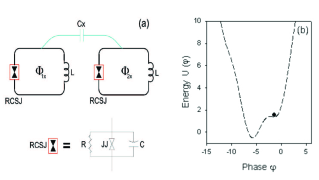
Figure 1: Equivalent circuit of capacitively coupled qubits. Each superconducting loop of inductance $L$ contains a Josephson junction modeled by the RCSJ subcircuit. (b) Potential energy (in units of $I_{C}\Phi_{0}/2\pi)$ of a superconducting loop interrupted by a Josephson junction as a function of the junction phase; the assumed normalized flux bias is 0.6941. The “virtual particle” representing the system is shown sitting at the bottom of its shallow well.

The experimental configuration of two coupled qubits is modeled with the equivalent circuit depicted in Fig.1(a). Each junction is characterized by a critical current $I_{c}$, resistance $R$, and capacitance $C$; each loop has an inductance $L$. The two loops, characterized by the Josephson phase variables $\varphi_{1}$ and $\varphi_{2}$, are coupled through a capacitance $C_{X}$. The externally applied fluxes through loops 1 and 2 are represented by $\Phi_{1x}$ and $\Phi_{2x}$. As discussed in [15], in dimensionless form the governing equations of this system turn out to be:

$$\ddot{\varphi}_{a}+\alpha\dot{\varphi}_{a}+\sin\varphi_{a}\cos\varphi_{b}=-\beta_{L}^{-1}\left[{\varphi_{a}+2\pi M_{a}}\right]$$ (1)

$$g^{-1}\ddot{\varphi}_{b}+\alpha\dot{\varphi}_{b}+\sin\varphi_{b}\cos\varphi_{a}=-\beta_{L}^{-1}\left[{\varphi_{b}+2\pi M_{b}}\right]\;,$$ (2)

with overdots denoting derivatives in dimensionless time $\tau=\omega_{J}t$. $\varphi_{a}=(\varphi_{1}+\varphi_{2})/2$ and $\varphi_{b}=(\varphi_{1}-\varphi_{2})/2$ are the transformed phase variables that are convenient for the analysis. The junction plasma frequency is $\omega_{J}=\sqrt{2eI_{c}/\hbar C}$; $\alpha=1/\omega_{J}CR$ and $\beta_{L}=2\pi LI_{c}/\Phi_{0}$, $\Phi_{0}=h/2e$ being the flux quantum. $g^{-1}=1+2\gamma_{x}$ with $\gamma_{x}=C_{x}/C$ representing the mutual coupling coefficient. $M_{ix}=\Phi_{ix}/\Phi_{0}$ is the total normalized applied flux through loop $i$; $M_{a}=\tfrac{1}{2}(M_{1x}+M_{2x})$ and $M_{b}=\tfrac{1}{2}(M_{1x}-M_{2x})$ are corresponding transformed normalized magnetic fields. As in [15], parameter values were set at $\alpha=5\times 10^{-5}$, $\beta_{L}=2.841$, $g=0.9954$, $I_{c}=1.1\mu A$, $C=1.3pF$, and $\omega_{J}^{-1}=0.02ns$. Both loops are biased with a dc flux $M_{ix}=0.6941$ (resonance $\approx 5.1$GHz) and with superimposed microwave (MW) pulses as shown in Fig.3(A) of Ref. [14].

Our previous work [15] outlined the dynamical modes exhibited by this system. One of these modes is consistent with the experimental observations and can be obtained in the linear limit of oscillation amplitude. Following Ref. [15], we therefore take $M_{b}=0$, $\alpha\approx 0$, and for small amplitude oscillations of $\varphi_{1}$ and $\varphi_{2}$, we write $\varphi_{a}=\varphi_{0}+\psi_{a}$, where $\varphi_{0}$ is a constant and $|\psi_{a}|\ll 1$. Similarly we assume $|\varphi_{b}|\ll 1$. Inserting this ansatz with $\alpha=0$ (for simplicity) gives the linear equations

$$\beta_{L}\sin\varphi_{0}+\varphi_{0}+2\pi M_{a} = 0$$ (3)

$$\ddot{\psi}_{a}+(\cos\varphi_{0}+\beta_{L}^{-1})\psi_{a} = 0$$ (4)

$$g^{-1}\ddot{\varphi}_{b}+(\cos\varphi_{0}+\beta_{L}^{-1})\varphi_{b} = 0\;.$$ (5)

The first of these equations provides the average phase $\varphi_{0}$ for each of the two loops given the external DC magnetic field. The next two equations have solutions $\psi_{a}=A\sin(\omega_{a}t+\theta_{a})$ and $\varphi_{b}=B\sin(\omega_{b}t+\theta_{b})$, where the four parameters, $A,B,$ $\theta_{a}$ and $\theta_{b}$ are given by initial conditions. The two resonance frequencies are $\omega_{a}^{2}=\cos\varphi_{0}+\beta_{L}^{-1}$ and $\omega_{b}=\sqrt{g}\omega_{a}$. The Josephson phases $\varphi_{i}$ of the two loops therefore evolve according to

$$\varphi_{i}-\varphi_{0}\;=\;\psi_{a}\pm\varphi_{b}$$ (6)

$$=\;\sqrt{A^{2}+B^{2}\pm 2AB\cos 2(\omega_{d}t+\theta_{d})}\sin(\omega_{s}t+\theta_{i})\;,$$

where $i=1,2$, and ”$+$” and ”$-$” apply to $i=1$ and $i=2$, respectively. The frequencies and phases are $\omega_{s}=\tfrac{1}{2}(\omega_{a}+\omega_{b})$, $\omega_{d}=\tfrac{1}{2}(\omega_{a}-\omega_{b})$, and $\theta_{d}=\tfrac{1}{2}(\theta_{a}-\theta_{b})$. This expression directly gives the experimentally [14] and theoretically [15] observed slow envelope modulation of the two coupled oscillators, and calculating the modulation frequency from the experimentally provided system parameters yields $\Omega_{I}=2\omega_{d}\approx 0.001455$, which is in very good agreement with observations [14,15]. The two phases $\theta_{1}$ and $\theta_{2}$ are also modulated with $\omega_{d}$ such that

$$\sin\theta_{i} = A\cos(\omega_{d}t+\theta_{a})\pm B\cos(\omega_{d}t-\theta_{b})$$ (7)

$$\cos\theta_{i} = -A\sin(\omega_{d}t+\theta_{a})\pm B\sin(\omega_{d}t-\theta_{b})\;.$$ (8)

We now discuss how these simple linear oscillations are related to the Bloch-vectors that have been used in the literature to illustrate the system behavior. In analogy with the quantum mechanical picture, we define a Bloch-sphere centered in a Cartesian coordinate system with a horizontal $xy$-plane and a vertical z-axis. The corresponding Bloch vector of an oscillator is given by the phase and amplitude of oscillation such that the phase of oscillation provides the direction in the xy-plane and the amplitude (or, equivalently, the energy) provides the $z$-coordinate. The definition of the vertical axis is given by the switching probabilities when the probe pulse is applied: $z=-1$ (vertical down) is a state with near-zero switching probability; $z=1$ (vertical up) is a state with near-unity switching probability; and $z=0$ (horizontal) are states with intermediate switching probability. In the present system of two coupled Josephson loops, the $z=0$ states (ideally 50% switching) are generated by initially applying a $\pi$-MW pulse of half a Rabi-period duration (notice that Rabi-type oscillations are already characterized in the classical system [13]) to one of the loops, then allowing the two coupled oscillators to exchange energy during a time of free evolution until their energy contents, and therefore switching probabilities, coincide (see Refs. [14,15]). Notice that the experiments can only measure the vertical axis $z$ by the switching probability. Thus, in order to experimentally gain any phase information from an oscillator (i.e., the xy-coordinate of the Bloch vector in the xy-plane), one must ”rotate” the Bloch vector $\tfrac{\pi}{2}$ around horizontal axes of the Bloch-sphere before conducting the measurement [14]. This is done by applying additional $\tfrac{\pi}{2}$-MW pulses of a duration that is about half of the initial $\pi$-MW pulse. The phase-difference between such rotation pulse and the perturbed oscillator determines if the oscillator energy is amplified ($z$ increases) or attenuated ($z$ decreases). Applying pulses of different phases can therefore illuminate the phase (the $xy$ coordinates) of a Bloch-vector by subsequent switching ($z$) measurements. A pair of two such orthogonal $\tfrac{\pi}{2}$ pulses are denoted $X$ and $Y$. This is the classical analog to state tomography.

We conduct state tomography by simultaneous switching measurements of the two loops after having applied rotation pulses $(I,X,Y)$. We acquire the probabilities in the form, where, e.g., $P_{X_{1}Y_{0}}$ is the probability for simultaneously measuring a switch in loop 1 and a no-switch in loop 2 after having applied an $X$-rotation to loop 1 and a $Y$-rotation to loop 2. The notation for not applying an $X$ or $Y$ rotation is $I$. Following the quantum mechanical treatment, these measured probabilities can be fed into expressions for the Hermitian density matrix $\{\rho_{jk}\}_{4\times 4}$ in, e.g., the following way: $\rho_{11}=P_{I_{0}I_{0}}$, $\rho_{22}=P_{I_{0}I_{1}}$, $\rho_{33}=P_{I_{1}I_{0}}$, $\rho_{44}=P_{I_{1}I_{1}}$, and

$$2\rho_{12} = (P_{I_{0}X_{1}}-P_{I_{0}X_{0}})+i(P_{I_{0}Y_{0}}-P_{I_{0}Y_{1}})$$ (9)

$$2\rho_{13} = (P_{X_{1}I_{0}}-P_{X_{0}I_{0}})+i(P_{Y_{0}I_{0}}-P_{Y_{1}I_{0}})$$ (10)

$$2\rho_{24} = (P_{X_{1}I_{1}}-P_{X_{0}I_{1}})+i(P_{Y_{0}I_{1}}-P_{Y_{1}I_{1}})$$ (11)

$$2\rho_{34} = (P_{I_{1}X_{1}}-P_{I_{1}X_{0}})+i(P_{I_{1}Y_{0}}-P_{I_{1}Y_{1}})$$ (12)

$$2\rho_{23} = (1-P_{X_{0}X_{1}}-P_{X_{1}X_{0}}-P_{Y_{0}Y_{1}}-P_{Y_{1}Y_{0}})$$

$$+ i(P_{Y_{0}X_{1}}+P_{Y_{1}X_{0}}-P_{X_{0}Y_{1}}-P_{X_{1}Y_{0}})$$

$$2\rho_{14} = (P_{Y_{0}Y_{1}}+P_{Y_{1}Y_{0}}-P_{X_{0}X_{1}}-P_{X_{1}X_{0}})$$

$$+ i(P_{X_{0}Y_{1}}+P_{X_{1}Y_{0}}+P_{Y_{0}X_{1}}+P_{Y_{1}X_{0}}-1)\;.$$

Our only deviation from the experimental work [14] is that we use the direct expressions above instead of a least-square fit.

Simulations were conducted as follows. Each loop was initially at rest in its shallow potential well generated by the DC magnetic field as illustrated in Fig.1(b). A $\pi$-MW pulse was applied with a randomly chosen phase and a normalized amplitude of $7.5\times 10^{-5}$ for 500 time units to loop 2. This elevates loop 2 to a relatively high energy state, while loop 1 is left near the bottom of its well. The free evolution of the system is therefore approximately given by Eq. (6) with $\theta_{d}\approx 0$ and $0\leq B\lesssim A$ after the initial $\pi$-MW field on loop 2 is terminated. The two coupled oscillators now evolve until a rotation pulse is applied to one or both of the oscillators, after which possible switching is measured by applying a probe pulse to each loop. The rotation pulses were chosen in accordance with the experiments with a duration of 200 time units and same amplitude as the initial $\pi$-MW pulse. Their phases were randomly chosen, but such that $X$ and $Y$ pulses were $\tfrac{\pi}{2}$ out of phase. The probe pulse was calibrated so that the initial state prior to MW pulses would yield vanishing switching probability, the state of loop 2 immediately following the initial $\pi$-MW pulse would result in near certain switching, and the states, where the energies of the two loops become equal, would result in some intermediate percentage of significance. Thus, we chose a half-sine wave with duration 500 time units and normalized amplitude $3.6\times 10^{-3}$. The energies of the two loops became equal at a time of approximately 900 units after the termination of the $\pi$-MW pulse, and the probe pulse was centered near this value. The $(I),X,Y$ rotation pulses were applied immediately prior to the application of the probe pulse. We repeated such simulations 2000 times with different values of the randomly chosen phases in order to obtain a set of switching probabilities for any given combination of rotation pulses. We then generated a density matrix from the simultaneous switching probabilities, as outlined above. A typical example of this is presented in Figure 2, where the real and imaginary parts of the matrix are shown separately. We note the striking resemblance to the density matrix that was previously published (Fig. 3B of Ref. [14]) based on the experimental data. The matrix shows relatively small real magnitudes outside the diagonal, and relatively small imaginary elements, except for $\rho_{23}$, which contain the signature of ”entanglement”. Thus, simulation data generated from the classical RCSJ model yields a density matrix that matches in its essential features the density matrix produced from experimental observations of the coupled qubit system. In order to emphasize the similarity between our result here and that of Ref. [14], we can calculate the “fidelity” $F_{\exp}=\sqrt{\nu^{\ast T}\rho_{data}\nu}$, where $\rho_{data}$ is the density matrix developed based on the acquired classical data and $\nu=(0,\tfrac{1}{\sqrt{2}},-\tfrac{i}{\sqrt{2}},0)^{T}$ is the vector corresponding to the ideally expected entangled state [5]. With the developed density matrix shown in Figure 2 we get $F_{\exp}=0.77$. This value is very close to the one obtained in Ref. [14], and we will now discuss this result.

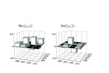
Figure 2: State tomography of “entangled” qubits. Real and imaginary components, respectively, of the density matrix. We deliberately choose the notation $|ij)$ rather than $|ij\rangle$ to distinguish our results as fundamentally classical rather than quantum mechanical. This density matrix should be compared to Fig. 3B of Ref. [14].

The probe pulse was calibrated to give approximately the same optimal switching probability for the two loops when no rotation pulses were applied. The implication of this is that the corresponding Bloch vectors would be positioned in the xy-plane of the Bloch sphere when these simultaneous measurements are conducted. The probability $P_{1}$ for switching a loop can therefore be related to the z-coordinate of the unit-Bloch-vector in the simple way $P_{1}=\tfrac{1}{2}(1+z)$. Correspondingly, if an $X$ or a $Y$ rotation is applied prior to the measurement, one would have the probabilities $P_{X_{1}}=\tfrac{1}{2}(1+\sin\theta)$ and $P_{Y_{1}}=\tfrac{1}{2}(1-\cos\theta)$, where $\theta$ is the angle (relative to the $x$-axis) of the Bloch-vector in the xy-plane prior to the application of a $\tfrac{\pi}{2}$ rotation pulse. Notice that the probability of switching in the classical system is given only by the sampling of the outcomes of random MW-phases (at the extreme low temperature limit), whereas the quantum mechanical picture sees the switching probability as only due to tunneling. In averaging over all random phases $\theta$, one can get a good sense of what to expect from the density matrix elements. For example the particular element $\rho_{23}$ corresponding to a random-phase averaged ensemble of two Bloch-vectors, which are $\Gamma=\theta_{1}-\theta_{2}$ out of phase in the xy-plane, we have $\rho_{23}=\tfrac{1}{4}\exp(i\Gamma)$. This explains the information that the density matrix provides. The important element $\rho_{23}$ is a measure of the angle $\Gamma$ between the two simultaneously detected Bloch-vectors in the xy-plane – or, equivalently, the phase difference between the Josephson phase oscillations of the two loops. If we produce an element $\rho_{23}\approx\pm\tfrac{i}{4}$ (which is what is obtained), then this arises from two vectors that are nearly orthogonal in the xy-plane – or, equivalently, that the oscillations of the two loops are $\tfrac{\pi}{2}$ out of phase. However, the formalism does not explain why this is, and the result may have nothing to do with quantum mechanics, as we have seen here.

The fact that the classical RCSJ model produces this particular result is not a coincidence. We concluded above that the $\pi$-MW initiation of the system provides for the parameters $0\leq B\lesssim A$ and $\theta_{d}\approx 0$. If we observe the system at the time $t_{m}$ when the two energies coincide ($\omega_{d}t_{m}=\tfrac{\pi}{4}$), we can see from equations (7) and (8) that $\Gamma=\theta_{1}-\theta_{2}=\tan^{-1}\tfrac{A-B}{A+B}-\tan^{-1}\tfrac{A+B}{A-B}$, which is $\Gamma=-\tfrac{\pi}{2}$ for $A=B$, and $\Gamma\gtrsim-\tfrac{\pi}{2}$ for $A\gtrsim B\geq 0$. Thus, the two coupled oscillators are naturally orthogonal in phase when their energy contents are similar, and the resulting density matrix, obtained from the switching measurements after rotations, therefore reflects this fact.

We have demonstrated that the classical RCSJ model of two coupled qubits exhibits the same signatures as observed experimentally when conducting state tomography and examining the resulting density matrix. These signatures have previously been used to argue for an unambiguous demonstration of quantum entanglement. However, given that our data are definitely classical in origin, we submit that such definite conclusions cannot be made. Instead, the density matrix, and the element $\rho_{23}$ in particular, provides information only about the phase difference between the Josephson oscillations of the two superconducting loops without providing the underlying reason for this phase difference. Assuming that the system is governed by quantum mechanics this may be interpreted as a signature of quantum entanglement. However, one does not need to assume this, and our classical analysis of the system has revealed that exactly the same signature in the density matrix appears as a result of the weak coupling. This leads to an ambiguous interpretation of the observed phenomena. We therefore conclude that unambiguous demonstrations of quantum behavior in this class of systems must be analyzed not only in light of the quantum mechanical model and its expectations, but also in light of what the corresponding classical model can predict and explain.

- (1) J. Bardeen, Phys. Rev. Lett. 42, 1498 (1979); R. E. Thorne, J. R. Tucker, and J. Bardeen, Phys. Rev. Lett. 58, 828 (1987).
- (2) L. Sneddon, M. C. Cross, and D. S. Fisher, Phys. Rev. Lett. 49, 292 (1982); R. A. Klemm and J. R. Schrieffer, Phys. Rev. Lett. 51, 47 (1983).
- (3) S. Pancharatnam, Proceedings of Indian Academic of Science, 44, A, 247 (1956).M. V. Berry, Proceedings of the Royal Society of London, A, 392, 45 (1984).
- (4) R. Y. Chiao, Phys. Rev. Lett. 57, 933 (1986); A. Tomita and R. Y. Chiao, Phys. Rev. Lett. 57, 937 (1986)
- (5) F. D. Haldane , Phys. Rev. Lett 59, 1788 (1987)
- (6) J. Segert, Phys. Rev. A 36, 10 (1987)
- (7) T. Van Duzer and C.W. Turner, Principles of Superconductive Devices and Circuits (Elsevier, New York,1981), Chapter 5.
- (8) P. W. Anderson, in Lectures on the Many Body Problem, Ed. by E. R. Caianiello (Academic Press NY 1964), Vol. 2, p. 132.
- (9) A. O. Caldeira and A. J. Leggett, Phys. Rev. Lett. 46, 211 (1981); A. J. Legget and A. Garg, Phys. Rev. Lett. 54, 857 (1985).
- (10) I. Affleck, Phys. Rev. Lett. 46, 388 (1981).
- (11) J.M. Martinis, M.H. Devoret, and J. Clarke, Phys. Rev. Lett. 55, 1543 (1985).
- (12) See, e.g., J.M. Martinis, S. Nam, J. Aumentado, and C. Urbina, Phys. Rev. Lett. 89, 117901 (2002); R.W. Simmonds, K.M. Lang, D.A. Hite, S. Nam, D.P. Pappas, and J.M. Martinis, Phys. Rev. Lett. 93, 077003 (2004); J. Claudon, F. Balestro, F.W.J. Hekking, and O. Buisson, Phys. Rev. Lett. 93 (2004); D. Vion, A. Aassime, A. Cottet, P. Joyez, H. Pothier, C. Urbina, D. Esteve, and M.H. Devoret, Forschr. Phys. 51, 462 (2003).
- (13) N. Grønbech-Jensen et al., Phys. Rev. Lett. 93, 107002 (2004); N. Grønbech-Jensen and M. Cirillo, Phys. Rev. Lett., 95 067001 (2005); J. E. Marchese, M. Cirillo, and N. Grønbech-Jensen, Phys. Rev. B 73, 174507 (2006); N. Grønbech-Jensen et al., “Anomalous thermal escape in Josephson systems perturbed by microwaves”, in Quantum Computing: Solid State Systems eds. B. Ruggiero, P. Delsing, C. Granata, Y. Paskin, and P. Silvestrini (Springer, New York, 2006), pp. 111-119; J. E. Marchese, M. Cirillo, and N. Grønbech-Jensen, Eur. Phys. J. 147, 333-342 (2007).
- (14) M. Steffen, M. Ansmann, R.C. Bialczak, N. Katz, E Lucero, R. McDermott, M. Neeley, E.M. Weig, A.N. Cleland, J.M. Martinis, Science 313, 1423 (2006).
- (15) J.A. Blackburn, J.E. Marchese, M. Cirillo, and N. Grønbech-Jensen, Phys. Rev. B 79, 054516 (2009).