Math. Model. Nat. Phenom.

Vol. 5, No. 3, 2010, pp. 146-184

Observers for Canonic Models of Neural Oscillators

D. Fairhurst^a, I. Tyukin ^a,c,d, H. Nijmeijer^b, and C. van Leeuwen^c

^a Department of Mathematics, University of Leicester, University Road, LE1 7RH, UK

^b Department of Mechanical Engineering, Eindhoven University of Technology,

P.O. Box 513 5600 MB, Eindhoven, The Netherlands

^c RIKEN (Institute for Physical and Chemical Research) Brain Science Institute,

2-1, Hirosawa, Wako-shi, Saitama, 351-0198, Japan

^d Deptartment of Automation and Control Processes, St-Petersburg State University

of Electrical Engineering, Prof. Popova str. 5, 197376, Russia

Abstract. We consider the problem of state and parameter estimation for a class of nonlinear oscillators defined as a system of coupled nonlinear ordinary differential equations. Observable variables are limited to a few components of state vector and an input signal. This class of systems describes a set of canonic models governing the dynamics of evoked potential in neural membranes, including Hodgkin-Huxley, Hindmarsh-Rose, FitzHugh-Nagumo, and Morris-Lecar models. We consider the problem of state and parameter reconstruction for these models within the classical framework of observer design. This framework offers computationally-efficient solutions to the problem of state and parameter reconstruction of a system of nonlinear differential equations, provided that these equations are in the so-called adaptive observer canonic form. We show that despite typical neural oscillators being locally observable they are not in the adaptive canonic observer form. Furthermore, we show that no parameter-independent diffeomorphism exists such that the original equations of these models can be transformed into the adaptive canonic observer form. We demonstrate, however, that for the class of Hindmarsh-Rose and FitzHugh-Nagumo models, parameter-dependent coordinate transformations can be used to render these systems into the adaptive observer canonical form. This allows reconstruction, at least partially and up to a (bi)linear transformation, of unknown state and parameter values with exponential rate of convergence. In order to avoid the problem of only partial reconstruction and at the same time to be able to deal with more general nonlinear models in which the unknown parameters enter the system nonlinearly, we present a new method for state and parameter reconstruction for these systems. The method combines advantages of standard Lyapunov-based design with more flexible design and analysis techniques based on the notions of positive invariance and small-gain theorems. We show that this flexibility allows to overcome ill-conditioning and non-uniqueness issues arising in this problem. Effectiveness of our method is illustrated with simple numerical examples.

Key words: Parameter estimation, adaptive observers, nonlinear parametrization, convergence, nonlinear systems, neural oscillators

AMS subject classification: 93B30, 93B10, 93B07, 93A30, 92B05

Notations and Nomenclature

The following notational conventions are used throughout the paper:

• $\mathbb{R}$ is the field of real numbers.

• $\mathbb{R}_{>0}=\{x\in\mathbb{R}\ |\ x>0\}$.

• $\mathbb{Z}$ denotes the set of integers, and $\mathbb{N}$ stands for the set of positive integers.

• The Euclidian norm of $x\in\mathbb{R}^{n}$ is denoted by $\left\|x\right\|$.

• $\mathcal{C}^{r}$ denotes the space of continuous functions that are at least $r$ times differentiable.

• Let $h:\mathbb{R}^{n}\rightarrow\mathbb{R}$ be a differentiable function and $f:\mathbb{R}^{n}\rightarrow\mathbb{R}^{n}$. Then $L_{f}h(x)$, or simply $L_{f}h$, is the Lie derivative of $h$ with respect to $f$:

  $$L_{f}h(x)=\frac{{\partial}h}{{\partial}x}f(x)$$

• Let $f,g:\mathbb{R}^{n}\rightarrow\mathbb{R}^{n}$ be differentiable vector-fields. Then the symbol $[f,g]$ stands for the Lie bracket:

  $$[f,g]=\frac{{\partial}f}{{\partial}x}g-\frac{{\partial}g}{{\partial}x}f$$

  The adjoint representation of the Lie bracket is defined as

  $$\mathrm{ad}_{f}^{0}g=g,\ \mathrm{ad}_{f}^{k}g=[f,\mathrm{ad}_{f}^{k-1}g]$$

• Let $\mathcal{A}$ be a subset of $\mathbb{R}^{n}$, then for all $x\in\mathbb{R}^{n}$, we define $\mathrm{dist}(\mathcal{A},x)=\inf_{q\in\mathcal{A}}\|x-q\|$.

• $\mathcal{O}(\cdot)$ denotes a function such that $\lim_{s\rightarrow 0}\mathcal{O}(s)/s=d$, $d\in\mathbb{R}$, $d\neq 0$.

• Finally, let $\epsilon\in\mathbb{R}_{>0}$, then $\left\|x\right\|_{\epsilon}$ stands for the following:

  $$\left\|x\right\|_{\epsilon}=\left\{\begin{array}[]{ll}\left\|x\right\|-\epsilon,&\left\|x\right\|>\epsilon,\\ 0,&\left\|x\right\|\leq\epsilon.\end{array}\right.$$

1. Introduction

Mathematical modelling of brain processes and function is recognized as an important tool of modern neuroscience [14]. It allows us to predict, analyze and understand intricate processes of neural computations, without invoking technically involving and costly experiments. Successful examples include but are not limited to modelling the memory function [4], [15] and the mechanisms of phase-resetting in olivo-cerebellar networks [38]. Availability of quantitatively accurate models of individual neural cells is an important prerequisite of such studies.

The majority of available models of individual biological neurons are the systems of ordinary differential equations describing the cell’s response to stimulation; their parameters characterize variables such as time constants, conductances, and response thresholds, important for relating the model responses to behavior of biological cells. Typically two general classes of models co-exist: phenomenological and mathematical ones. Models of the first class, such as e.g. the Hodgkin-Huxley equations, claim biological plausibility, whereas models of the second class are more abstract mathematical reductions without explicit relation of all of their variables to physical quantities such as conductances and ionic currents (see Table 1).

Table 1: Examples of typical mathematical models of spiking single neurons. Biologically plausible equations of membrane potential generation in a giant axon of a squid (left panel), and a reduction of these equations to an oscillator with polynomial right-hand side (right panel)

Hodgkin-Huxley Model [10]

Hindmarsh-Rose Model [9]

$\displaystyle\dot{v}$ $\displaystyle=$ $\displaystyle I(t)-\left[\theta_{1}m^{3}h(v+\theta_{2})+\theta_{3}n^{4}(v+\theta_{4})+\theta_{5}v+\theta_{6}\right]$ $\displaystyle\dot{m}$ $\displaystyle=$ $\displaystyle(1-m)\varphi\left(\frac{v+\theta_{7}}{\theta_{8}}\right)-m\ \theta_{9}\exp\frac{v}{\theta_{10}}$ $\displaystyle\dot{n}$ $\displaystyle=$ $\displaystyle(1-n)\theta_{11}\varphi\left(\frac{v+\theta_{12}}{\theta_{13}}\right)-n\ \theta_{14}\exp\frac{v}{\theta_{15}}$ (1.1) $\displaystyle\dot{h}$ $\displaystyle=$ $\displaystyle(1-h)\theta_{16}\exp\frac{v}{\theta_{17}}-h/\left(1+\exp\frac{v+\theta_{18}}{\theta_{19}}\right)$ $\varphi(x)={x}/({\exp{x}-1})$, $\theta_{1},...,\theta_{19}$ – parameters, $I:\mathbb{R}\rightarrow\mathbb{R}$ – input current

$\displaystyle\dot{v}$ $\displaystyle=$ $\displaystyle\theta_{1}(\theta_{2}r-f(v))+I(t)$ $\displaystyle\dot{r}$ $\displaystyle=$ $\displaystyle\theta_{3}(g(v)-\theta_{4}r)$ (1.2) $f(v)$ and $g(v)$ are polynomials: $\displaystyle f(v)$ $\displaystyle=$ $\displaystyle\theta_{5}+\theta_{6}v+$ $\displaystyle=$ $\displaystyle\theta_{7}v^{2}+\theta_{8}v^{3};$ $\displaystyle g(v)$ $\displaystyle=$ $\displaystyle\theta_{9}+\theta_{10}v+\theta_{11}v^{2}$ $I:\mathbb{R}\rightarrow\mathbb{R}$ is the external input, $\theta_{1},...,\theta_{11}$ – parameters

Despite these differences, these models admit a common general description which will be referred to as canonic. In particular, the dynamics of a typical neuron are governed by the following set of equations

$$\begin{split}\dot{v}&={\sum}_{j}\ \varphi_{j}(v,t)p_{j}(r)\theta_{j}+I(t);\\ \dot{r}_{i}&=-a_{i}(v,\theta,t)r_{i}+b_{i}(v,\theta,t);\\ \theta&=(\theta_{1},\theta_{2},\dots).\end{split}$$ (1.3)

in which the variable $v$ is the membrane potential, and $r_{i}$ are the gating variables of which the values are not available for direct observation. Functions $\varphi_{j}(\cdot,\cdot)$, $p_{j}(\cdot)\in\mathcal{C}^{1}$ are assumed to be known; they model components of specific ionic conductances. Functions $a_{i}(\cdot)$, $b_{i}(\cdot)\in\mathcal{C}^{1}$ are also known, yet they depend on the unknown parameter vector $\theta$. System (1.3) is a typical conductance-based description of the evoked potential generation in neural membranes [13]. It is also an obvious generalization of many purely mathematical models of spike generation such as the FitzHugh-Nagumo [7] or the Hindmarsh-Rose equations [9]. In this sense systems (1.3) represent typical building blocks in the modelling literature.

In order to be able to model the behavior of large numbers of individual cells of which the input-output responses are described by (1.3), computational tools for automated fitting of models of neurons to data are needed. These tools are the algorithms for state and parameter reconstruction of (1.3) from the available measurements of $v(t)$ and $I(t)$ over time.

Fitting parameters of nonlinear ordinary differential equations to data is recognized as a hard computational problem [5] that “has not been yet treated in full generality” [20]. Within the field of neuroscience, conventional methods for fitting parameters of model neurons to measured data are often restricted to hand-tuning or exhaustive trial-and-error search in the space of model parameters [31]. Even though these strategies allow careful and detailed exploration in the space of parameters they suffer from the same problem – the curse of dimensionality.

Available alternatives, recognizing obvious nonlinearity of the original problem, propose to reformulate the original estimation problem as that of searching for the parameters of a system of difference equations approximating solutions of (1.3) [1]; or predominantly offer search-based optimization heuristics (see [37] for a detailed review) as the main tool for automated fitting of neural models. Straightforward exhaustive-search approaches however are limited to varying only few model parameters over sparse grids, e.g. as in [31] where $8$ parameters were split into $6$ bands. Coarseness of this parametrization leads to non-uniqueness of signal representation, leaving room for uncertainty and inability to distinguish between subtle changes in the cell. More fine-grained search algorithms are currently infeasible, technically speaking. Other heuristics, such as evolutionary algorithms, are examined in [2]. According to [2], replacing exhaustive search with evolutionary algorithms allows to increase the number of varying parameters to $24$. Yet, computational complexity of the problem still delimits the search to sparse grids ($6$ bands per single parameter) and requires days of simulation by a cluster of $10$ Apple 2.3 GHz nodes. Furthermore, because all these strategies are heuristic, accuracy of final results is not guaranteed.

The main aim of this article is to present a feasible substitute to these heuristic strategies for automatic reconstruction of state and parameters of canonic neural models (1.3). To develop computationally efficient procedures for state and parameter reconstruction of (1.3) we propose to exploit the wealth of system-identification and estimation approaches from the domain of control theory. These approaches are based on the system-theoretic concepts of observability and identifiability [30], [12],[19] from control theory, and the notions of Lyapunov stability [22] and weakly attracting sets [26]. The advantage of using these approaches is that there is an abundance of algorithms (observers) already developed within the domain of control. These algorithms guarantee asymptotic and stable reconstruction of unmeasured quantities from the available observations, provided that the system equations are in an adaptive observer canonical form. Moreover, this reconstruction can be made exponentially fast without the need of substantial computational recourses. We study if system (1.3) is at all observable with respect to the output $v$, that is if its state and parameters can be reconstructed from observations of $v$. We present and analyze typical algorithms (adaptive observers) that are available in the literature. We show that for a large class of mathematical models of neural oscillators at least a part of the model parameters can be reconstructed exponentially fast.

In order to deal with more general classes of models and also to recover the rest of the model parameters we introduce a novel observer scheme. This scheme benefits from 1) the efficiency of uniformly converging estimation procedures (stable observers), 2) success of explorative search strategies in global optimization by allowing unstable convergence along dense trajectories, and 3) the power of qualitative analysis of dynamical systems. We present a general description of this observer and list its asymptotic properties. The theory of this new class of algorithms is based on the results of our previous studies in the domain of unstable convergence [35], [36]. We will present examples to demonstrate the performance of these algorithms.

The paper is organized as follows. In Section 2 we provide the basic notions of observability from the domain of mathematical control, test if typical canonical neural oscillators are observable, and present two major classes of systems (canonical forms) for which computationally efficient reconstruction procedures are available. In Section 3 we analyze the applicability of standard observers to the problem of reconstructing all unmeasured variables and parameters of typical models of neurons. We present two special cases in which such reconstruction is possible. In Section 4 we provide a description and asymptotic properties of our algorithm that applies to the most general subset of models (1.3). Section 5. contains examples of application of the considered observers, and Section 5 concludes the paper. Proofs of the main technical statements are presented in the Appendix.

2. Observer-based approaches to the problem of state and parameter estimation

Let us consider the following class of dynamical systems

$$\begin{split}\dot{x}&=f(x,\theta)+g(x,\theta)u(t),\quad x(t_{0})\in\Omega_{x}\subset\mathbb{R}^{n}\\ y&=h(x),\quad x\in\mathbb{R}^{n},\quad\theta\in\mathbb{R}^{d},\quad y\in\mathbb{R}\end{split}$$ (2.1)

where $f,g:\mathbb{R}^{n}\times\mathbb{R}^{m}\rightarrow\mathbb{R}^{n}$, $h:\mathbb{R}^{n}\rightarrow\mathbb{R}$ are smooth functions, and $u:\mathbb{R}\rightarrow\mathbb{R}$. Variable $x$ stands for the state vector, $u\in\mathcal{U}\subset C^{1}[t_{0},\infty)$ is the known input, $\theta\in\mathbb{R}^{m}$ is the vector of unknown parameters, and $y$ is the output of (2.1). System (2.1) includes equations (1.3) as a subclass and in this respect can be considered as plausible generalizations. Obviously, conclusions about (2.1) should be valid for systems (1.3) as well.

Given that the right-hand side of (2.1) is differentiable, for any $x^{\prime}\in\Omega_{x}$, $u\in\mathcal{C}^{1}[t_{0},\infty)$ there exists a time interval $\mathcal{T}=[t_{0},t_{1}]$, $t_{1}>t_{0}$ such that a solution $x(t,x^{\prime})$ of (2.1) passing through $x^{\prime}$ at $t_{0}$ exists for all $t\in\mathcal{T}$. Hence $y(t)=h(x(t))$ is defined for all $t\in\mathcal{T}$. For the sake of convenience we will assume that the interval $\mathcal{T}$ of the solutions is large enough or even coincides with $[t_{0},\infty)$ when necessary.

We are interested in finding an answer to the following question: suppose that we are able to measure the values of $y(t)$ and $u(t)$ precisely; wether and how the values of $x^{\prime}$ and parameter vector $\theta$ can be recovered from the observations of $y(t)$ and $u(t)$ over a finite subinterval of $\mathcal{T}$? A natural framework to answer to these questions is offered by the concept of observability [30].

Definition 1 (Observability).

Two states $x_{1},x_{2}\in\mathbb{R}^{n}$ are said to be indistinguishable (denoted by $x_{1}\mathcal{I}x_{2}$) for (2.1) if for every admissible input function $u$ the output function $t\rightarrow y(t,0,x_{1},u)$, $t\geq 0$ of the system for initial state $x(0)=x_{1}$, and the output function $t\rightarrow y(t,0,x_{2},u)$, $t\geq 0$ of the system for initial state $x(0)=x_{2}$, are identical on their common domain of definition. The system is called observable if $x_{1}\mathcal{I}x_{2}$ implies $x_{1}=x_{2}$.

According to Definition 1, observability of a dynamical system implies that the values of its state, $x(t)$, $t\in[t_{1},t_{2}]$ are completely determined by inputs and outputs $u(t)$, $y(t)$ over $[t_{1},t_{2}]$. Although this definition does not account for any unknown parameter vectors, one can easily see that the very same definition can be used for parameterized systems as well. Indeed, extending original equations (2.1) by including parameter vector $\theta$ as a component of the extended state vector $\tilde{x}=(x,\theta)^{T}$ results in

$$\begin{split}\dot{x}&=f(x,\theta)+g(x,\theta)u(t),\\ \dot{\theta}&=0\\ y&=h(x),\quad x(t_{0})\in\Omega_{x}\subset\mathbb{R}^{n}\end{split}$$ (2.2)

or, similarly, in

$$\begin{split}\dot{\tilde{x}}&=\tilde{f}(\tilde{x})+\tilde{g}(\tilde{x})u(t)\\ y&=\tilde{h}(\tilde{x}),\quad\tilde{x}(t_{0})=(x(t_{0}),\theta)^{T}\in\Omega_{\tilde{x}}\subset\mathbb{R}^{n+d}\end{split}$$ (2.3)

where $\tilde{f}(\tilde{x})=(f(x,\theta),0)^{T}$, $\tilde{g}(\tilde{x})=(g(x,\theta),0)^{T}$, and $\tilde{h}(\tilde{x})=(h(x),0)$. All uncertainties in (2.1), (2.2), including the parameter vector $\theta$, are now combined into the state vector of (2.3). Hence the problem of state and parameter reconstruction of (2.1) can be viewed as that of recovering the values of state for (2.3).

Definition 1 characterizes observability as a global property of a dynamical system. Sometimes, however, global observability of a system in $\mathbb{R}^{n}$ is not necessarily needed. Instead of asking if every point in the system’s state space is distinguishable from any other point it may be sufficient to know if the system’s states are distinguishable in some neighborhood of a given point. This necessitates the notion of local observability [30].

Let $V$ be an open subset of $\mathbb{R}^{n}$. Two states $x_{1},x_{2}\in V$ are said to be indistinguishable (denoted by $x_{1}\mathcal{I^{V}}x_{2}$) on $V$ for (2.1) if for every admissible input function $u:[0,T]\rightarrow\mathbb{R}$ with the property that the solutions $x(t,0,x_{1},u)$, and $x(t,0,x_{2},u)$ both remain in $V$ for $t\leq T$ the output function $t\rightarrow y(t,0,x_{1},u)$, $t\geq 0$ of the system for initial state $x(0)=x_{1}$, and the output function $t\rightarrow y(t,0,x_{2},u)$, $t\geq 0$ of the system for initial state $x(0)=x_{2}$, are identical for $0\leq t\leq T$ on their common domain of definition.

Definition 2 (Local observability [30]).

The system is called locally observable at $x_{0}$ if there exists a neighborhood $W\subset\mathbb{R}^{n}$ of $x_{0}$ such that for every neighborhood $V\subset W$ of $x_{0}$ the relation $x_{0}\mathcal{I^{V}}x_{1}$ implies $x_{0}=x_{1}$. The system is locally observable if it is observable at each $x_{0}$.

A number of observability tests are available that, given the functions ${h}$, ${f}$ in the right-hand side of (2.3), indicate if a given system is observable. Particular formulations of these tests may vary depending on whether e.g. the functions $f,g$ are analytic or time-invariant (inputs are constants).

In this article we will restrict our attention to those systems (2.2) in which the inputs $u(t)$ are constants. In this case we can replace the function $u(t)$ with an unknown parameter, and system (2.2) can be viewed as a system (2.3) yet without inputs. One of the most common observability tests for this class of autonomous systems is given below (see also [30], Theorem 3.32):

Proposition 3 (Observability test (Corollary 3.33, [30])).

System (2.3) is locally observable at a point $x^{o}\in U\subset\mathbb{R}^{n+d}$ if

$${\rm rank}\frac{\partial}{\partial\tilde{x}}\left(\tilde{h}(\tilde{x})\quad L_{\tilde{f}}\tilde{h}(\tilde{x})\quad L^{2}_{\tilde{f}}\tilde{h}(\tilde{x})\quad...\quad L^{n+d-1}_{\tilde{f}}\tilde{h}(\tilde{x})\right)^{T}=n+d,\quad\forall\ \tilde{x}\in U$$ (2.4)

In what follows we shall use the test above to determine if the models of neural dynamics are at all observable.

2.1. Local observability of neural oscillators

We start our observability analysis by applying the local observability test (2.4) to the Hindmarsh-Rose model (1). In order to do so we shall extend the system state space so that unknown parameters are the components of the extended state vector. In the case of the Hindmarsh-Rose model this procedure leads to the following extended system of equations:

$$\left(\begin{array}[]{c}\dot{x}_{1}\\ \dot{x}_{2}\\ \dot{\theta}_{13}\\ \dot{\theta}_{12}\\ \dot{\theta}_{11}\\ \dot{\theta}_{10}\\ \dot{\theta}_{22}\\ \dot{\theta}_{21}\\ \dot{\lambda}\end{array}\right)=\left(\begin{array}[]{c}\theta_{13}x_{1}^{3}+\theta_{12}x_{1}^{2}+\theta_{11}x_{1}+\theta_{10}+x_{2}\\ -\lambda x_{2}+\theta_{22}x_{1}^{2}+\theta_{21}x_{1}\\ 0\\ 0\\ 0\\ 0\\ 0\\ 0\\ 0\end{array}\right)$$ (2.23)

To test if there are points of local observability of system (2.23) it is sufficient to find a point in the state space of (2.23) at which the rank condition (2.4) holds. Here we computed the determinant:

$$\begin{split}D(\tilde{x})&=\frac{\partial}{\partial\tilde{x}}\left(h(\tilde{x})\quad L_{f}h(\tilde{x})\quad L^{2}_{f}h(\tilde{x})\quad...\quad L^{n-1}_{f}h(\tilde{x})\right)^{T}\\ \tilde{x}&=(x_{1},x_{2},{\theta}_{13},{\theta}_{12},\dot{\theta}_{11},{\theta}_{10},{\theta}_{22},\theta_{21},{\lambda})^{T}\end{split}$$

on a sparse grid (of $101\times 101$ pixels) and plotted those regions for which the determinant is less than a certain value, $\delta$. The neuron parameters were set to $L=-2,\theta_{13}=-10,\theta_{12}=-4,\theta_{11}=6,\theta_{10}=1,\theta_{22}=-32,\theta_{21}=-32$. Figure 1 shows results (obtained using Maple) for various values of $\delta$. The shaded regions correspond to the domains where $D(\tilde{x})<\delta$. According to these results, when the value of delta is made sufficiently small, condition $D(\tilde{x})>\delta$ holds for almost all points in the grid. This suggests that there are domains in which model (1) is indeed at least locally observable.

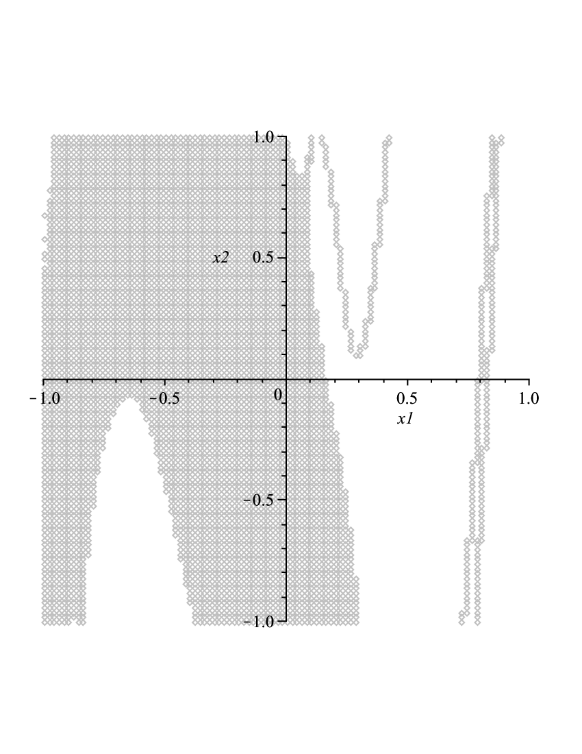
(a) $\delta=10^{20}$

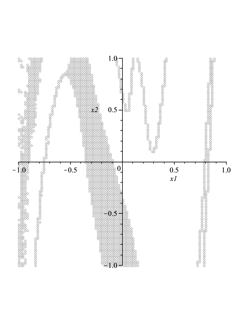
(b) $\delta=10^{15}$

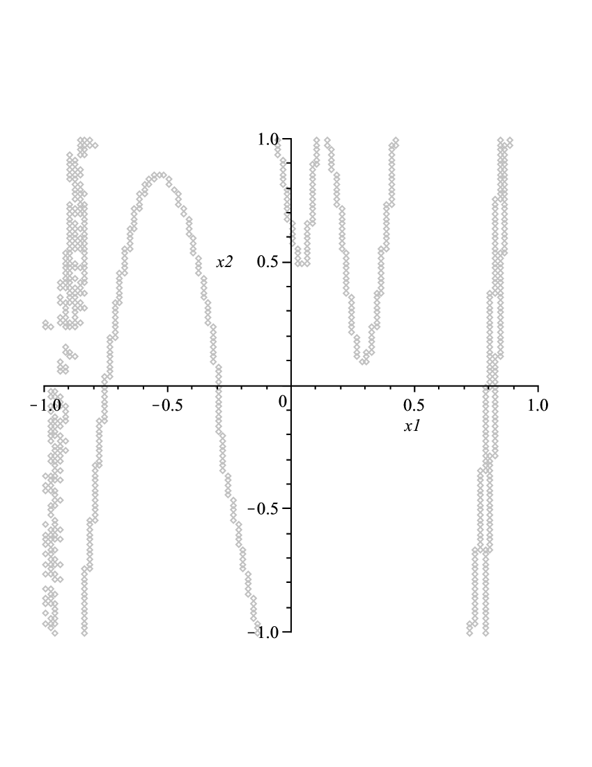
(c) $\delta=10^{5}$

Figure 1: Observability tests for Hindmrsh-Rose model neuron (1)

Let us now consider a more realistic, with respect to biological plausibility, set of equations. One of the simplest models of this type is the Morris-Lecar system [28]:

$$\begin{array}[]{c}\dot{v}(t)=-g_{Ca}\left(\frac{1}{2}+\frac{1}{2}\tanh\left(\frac{v(t)+1}{E_{4}}\right)(v(t)-E_{1})\right)-g_{K}w(t)(v(t)-E_{2})-g_{m}(v(t)-E_{3})\\ \dot{w}(t)=\frac{1}{5}\left(\frac{1}{2}+\frac{1}{2}\tanh\left(\frac{v(t)+1}{E_{5}}\right)-w(t)\right)\cosh\left(\frac{v(t)}{E_{6}}\right)\\ E_{1}=100,E_{2}=-70,E_{3}=-50,E_{4}=15,E_{5}=30,E_{6}=60,g_{Ca}=1.1,g_{K}=2.0,g_{m}=0.5\end{array}$$ (2.27)

As in the previous example we extend the system state space by considering unknown parameter as components of the extended state vector. This extension procedure results in the following set of equations:

$$\begin{split}&\left(\begin{array}[]{c}\dot{v}(t)\\ \dot{w}(t)\\ \dot{g}_{Ca}(t)\\ \dot{g}_{K}(t)\\ \dot{g}_{m}(t)\\ \dot{\lambda}(t)\end{array}\right)=\left(\begin{array}[]{c}-g_{Ca}\left(\frac{1}{2}+\frac{1}{2}\tanh\left(\frac{v+1}{15}\right)(v-100)\right)-g_{k}w(v+70)-g_{m}(v+50)\\ \frac{1}{5}\left(\frac{1}{2}+\frac{1}{2}\tanh\left(\frac{v+1}{30}\right)-w\right)\cosh\left(\frac{v}{60}\right)\\ 0\\ 0\\ 0\\ 0\end{array}\right)\end{split}$$

For this extended set of equations we estimated the regions where value of $D(x)$ exceeds some given $\delta>0$. These regions for different values of $\delta$ are presented in figure 2

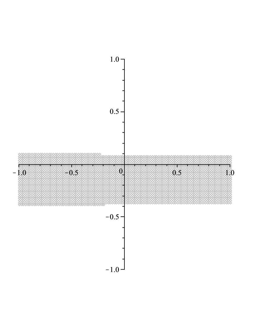
(a) $\delta=10000$

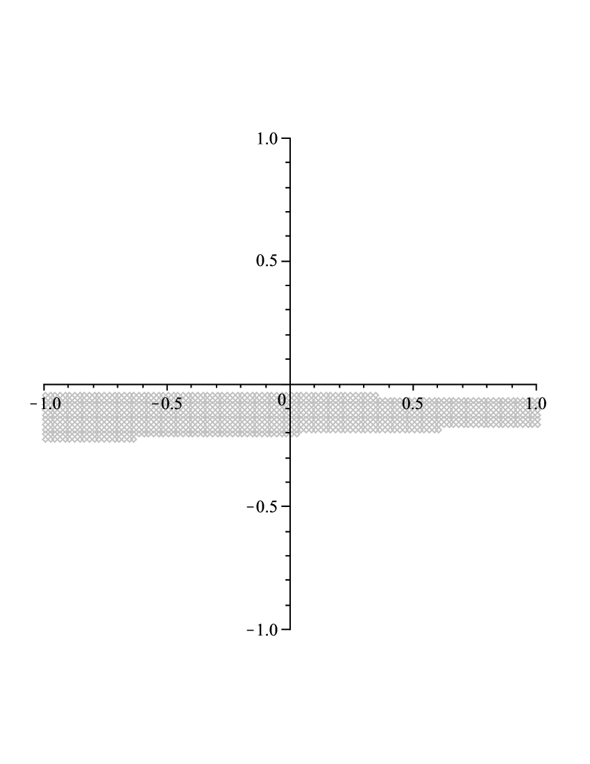
(b) $\delta=1000$

(c) $\delta=100$

Figure 2: Observability tests for Morris-Lecar model neuron

These results demonstrate that the Morris-Lecar system (2.27) is also locally observable.

As we have seen above, a fairly wide class of canonical mathematical and conductance-based models of evoked responses in neural membranes satisfy local observability conditions. We may thus expect to be able to solve the reconstruction problem for these models. In fact, as we show below in Sections 3, 4, the reconstruction problem can indeed be resolved efficiently at least for a part of unmeasured variables of the system. However, before we proceed with detailed description of these reconstruction algorithms, let us first review classes of systems for which solutions to the problem of exponentially fast reconstruction of all components of state and parameter vectors are already available in the literature.

2.2. Bastin-Gevers canonical form

We start with a class of systems comprising of a linear time-invariant part of which the equations are known and an additive time-varying component with linear parametrization. Parameters of this time-varying component are assumed to be uncertain. This class of systems was presented by G. Bastin and M. Gevers in 1989, [3], and its general form is as follows:

$$\begin{split}\dot{x}&=Rx+\Omega(t)\theta+g(t)\\ R&=\left(\begin{array}[]{cc}0&k^{T}\\ 0&F\end{array}\right)\ \Omega(t)=\left(\begin{array}[]{c}\Omega_{1}(t)\\ \overline{\Omega}(t)\end{array}\right)\\ y(t)&=x_{1}(t)\end{split}$$ (2.28)

In (2.28), $x\in\mathbb{R}^{n}$ is the state vector with $y=x_{1}$ assigned to be the output. $\theta\in\mathbb{R}^{p}=(\theta_{1},\cdot\cdot\cdot,\theta_{p})^{T}$ is the vector of unknown parameters. $R$ is a known matrix of constants where $k^{T}=(k_{2},\cdot\cdot\cdot,k_{n})$ and $F$ has dimension $(n-1)\times(n-1)$ with eigenvalues in the open left half plane. $\Omega(t)\in\mathbb{R}^{n\times p}$ is an $n\times p$ matrix of known functions of $t$; the first row is designated $\Omega_{1}$ and the remaining $n-1$ rows $\overline{\Omega}$. The vector function $g(t):\mathbb{R}\to\mathbb{R}^{n}$ is known.

Equations (2.28) are often referred to as an adaptive observer canonical form. This is because, subject to some mild non-degeneracy conditions, it is always possible to reconstruct the vector of unknown parameters $\theta$ and state $x$ from observations of $y$ over time. Moreover, the reconstruction can be made exponentially fast. Shown below is the adaptive observer presented in [3]. The system to be observed, state estimator, parameter adaption, auxiliary filter and regressor are given in equations (2.28), (2.31), (2.32), (2.33), (2.34) respectively

$$\dot{\hat{x}}(t) = R\hat{x}(t)+\Omega(t)\hat{\theta}+g(t)+\left(\begin{array}[]{c}c_{1}\tilde{y}\\ V(t)\dot{\hat{\theta}}\end{array}\right)$$ (2.31)

$$\dot{\hat{\theta}}(t) = \Gamma\varphi(t)\tilde{y}(t)$$ (2.32)

$$\dot{V}(t) = FV(t)+\overline{\Omega}(t),\quad V(0)=0$$ (2.33)

$$\varphi(t) = V^{T}(t)k+\Omega_{1}^{T}(t)$$ (2.34)

The output is $y=x_{1}$, its estimate is $\hat{y}=\hat{x}_{1}$ and its error is $\tilde{y}=y-\hat{y}$. This observer contains some parameters of its own which are at the design’s disposal. $\Gamma=\Gamma^{T}$ is an arbitrary positive definite matrix, normally chosen as $\Gamma=\textrm{diag}(\gamma_{1},\gamma_{2},...,\gamma_{p})$, $\gamma_{i}>0$. $c_{1}>0$. The auxiliary filter $V(t)$ is an $(n-1)\times p$ matrix and $\varphi(t)$ is a $p$ vector.

Using the transformation (2.38), the error system (2.45) is obtained.

$$\begin{array}[]{c}\tilde{x}^{*}=\tilde{x}-\left(\begin{array}[]{c}0\\ V\tilde{\theta}\end{array}\right),\ \tilde{x}=x-\hat{x}\end{array}$$ (2.38)

$$\begin{array}[]{c}\dot{\tilde{x}}^{*}=\left(\begin{array}[]{cc}-c_{1}&k^{T}\\ 0&F\end{array}\right)\tilde{x}^{*}+\left(\begin{array}[]{c}\varphi^{T}\tilde{\theta}\\ 0\end{array}\right)\\ \dot{\tilde{\theta}}=-\Gamma\varphi\tilde{x}_{1}^{*}\end{array}$$ (2.45)

It is shown in [3], for constant unknown parameters, that the solution $x(t)=\hat{x}(t)$, $\theta=\hat{\theta}(t)$ of the extended system (2.31), (2.32), (2.33), (2.34) is globally exponentially stable provided certain conditions on the regressor vector, $\varphi(t)$, are met. These conditions are:

• the regressor vector $\varphi(t)$ is bounded for all $t\geq 0$

• $\dot{\varphi}(t)$ is bounded for all $t\geq 0$ except possibly at a countable number of points $\{t_{i}\}$ such that $\mathrm{min}|t_{i}-t_{j}|\geq\triangle>0$ for some arbitrary fixed $\triangle$.

• $\varphi(t)$ is persistently exciting: that is, there exists positive constant $\alpha,T$ such that for all $t_{0}\geq 0$

  $$\int_{t_{0}}^{t_{0}+T}\varphi(t)\varphi^{T}(t)\,\mathrm{d}t\geq\alpha I>0$$ (2.46)

Formally, asymptotic properties of observer (2.31), (2.32) are specified in the theorem below [3]

Theorem 4.

Suppose that

• $c_{1}>0$ and $F$ is a Hurwitz matrix, that is its eigenvalues belong to the left half of the complex plane;

• the function $\varphi(t)$ is globally bounded in $t$, and its time derivative exists and is globally bounded for all $t\geq 0$;

• the function $\varphi(t)$ is persistently exciting.

Then the origin of (2.45) is globally exponentially asymptotically stable.

Adaptive observer canonical form (2.28) applies to systems in which the regressor $\Omega(t)\theta$ does not depend explicitly on the unmeasured components of the state vector. The question, however, is when a rather general nonlinear system can be transformed into the proposed canonical form. This question was addressed in [24] in which a modified adaptive observer canonical form was proposed together with necessary and sufficient conditions describing when a given system can be transformed into such form via a diffeomorphic coordinate transformation. This canonical form is described in the next subsection.

2.3. Marino-Tomei canonical form

The canonical form presented in [24] is now shown here. The system to be observed (2.58), state estimator (2.59) and parameter adaption (2.60) are given below

$$\begin{array}[]{rcl}\dot{x}(t)&=&A_{1}x(t)+\phi_{0}(y(t),u(t))+b\sum_{i=1}^{p}\beta_{i}(y(t),u(t))\theta_{i}\\ y(t)&=&C_{1}x(t)\\ A_{1}&=&\left(\begin{array}[]{ccccc}0&1&0&...&0\\ 0&0&1&...&0\\ .&.&.&...&0\\ 0&0&0&...&1\\ 0&0&0&...&0\end{array}\right)\\ C_{1}&=&\left(\begin{array}[]{ccccc}1&0&0&...&0\end{array}\right)\\ &&x(t)\in\mathbb{R}^{n},y(t)\in\mathbb{R},\beta_{i}(\cdot,\cdot):\mathbb{R}\times\mathbb{R}\to\mathbb{R}\end{array}$$ (2.58)

In (2.58) $x(t)\in\mathbb{R}^{n}$ is the state vector with $x_{1}(t)$ assigned to be the output $y$. Matrices $A_{1},C_{1}$ are in canonical observer form. $\theta\in\mathbb{R}^{p}=(\theta_{1},\cdot\cdot\cdot,\theta_{p})^{T}$ is the vector of unknown parameters. The functions $\beta_{i}$ are known, bounded and piecewise continuous functions of $y(t),u(t)$. The column vector $b\in\mathbb{R}^{n}$ is assumed to be Hurwitz with $b_{1}\neq 0$.

Shown below is the adaptive observer presented in [24]

$$\dot{\hat{x}}(t) = (A_{1}-KC_{1})\hat{x}(t)+\phi_{0}(y(t),u(t))+b\sum_{i=1}^{p}\beta_{i}(y(t),u(t))\hat{\theta}_{i}+Ky(t)$$ (2.59)

$$\dot{\hat{\theta}} = \Gamma\beta(t)(y-C_{1}\hat{x})\mathrm{sign}(b_{1})$$ (2.60)

$$K = \frac{1}{b_{n}}(A_{1}b+\lambda b)=(k_{1},\cdot\cdot\cdot,k_{n})^{T}$$ (2.61)

with $\Gamma$ an arbitrary symmetric positive definite matrix and $\lambda$ an arbitrary positive real. The $n\times 1$ vector, $b$, is Hurwitz with $b_{n}\neq 0$.

For the more general case where the vector $b$ is an arbitrary vector, an observer is presented in [25].

Theorem 5.

[23] There exists a local change of coordinates, $z=\Phi(x)$, transforming

$$\dot{x} = f(x)+\sum_{i=1}^{p}\theta_{i}(t)q_{i}(x),\quad y=x_{1}$$ (2.62)

$$x\in\mathbb{R}^{n},y\in\mathbb{R},\theta_{i}\in\mathbb{R},q_{i}:\mathbb{R}^{n}\to\mathbb{R}^{n},n\geq 2$$

with $h(x^{o})=0$ and $(f,h)$ an observable pair, into the system

$$\dot{z} = A_{1}z+\psi(y)+\sum_{i=1}^{p}\theta_{i}(t)\psi_{i}(y),\quad y=C_{1}z$$ (2.63)

$$z\in\mathbb{R}^{n},\psi_{i}:\mathbb{R}\to\mathbb{R}^{n}$$

with $(A_{1},C_{1})$ in canonical observer form (2.58), if and only if

• $[ad_{f}^{i}g,ad_{f}^{j}g]=0,\quad 0\leq i,j\leq n-1$

• $[q_{i},ad_{f}^{j}g]=0,\quad 0\leq j\leq n-2,\quad 1\leq i\leq p$

where the vector field, $g(x)$, is uniquely defined by

$$\left\langle\frac{{\partial}}{{\partial}x}\left(\begin{array}[]{c}h(x)\\ L_{f}h(x)\\ ...\\ L_{f}^{n-1}h(x)\end{array}\right),g(x)\right\rangle=\left(\begin{array}[]{c}0\\ 0\\ ...\\ 1\end{array}\right)$$ (2.72)

The proof of this result is made along the following lines. Suppose we use the change of coordinates: $z=\Phi(x)$, then we have

$$\dot{z} = \frac{\partial\Phi}{\partial x}\dot{x}$$ (2.73)

$$= \left(\frac{\partial\Phi}{\partial x}f(x)\right)_{x=\Phi^{-1}(z)}+\frac{\partial\Phi}{\partial x}\sum_{i=1}^{p}\theta_{i}q_{i}(x)$$ (2.74)

It is shown in [23] that providing we meet the constraint:

$$[ad_{f}^{i}g,ad_{f}^{j}g]=0,\quad\forall x\in U,0\leq i,j\leq n-1$$ (2.75)

then we can cast the system into the adaptive observer canonical form

$$\dot{z} = A_{1}z+\psi(y)+\sum_{i=1}^{p}\frac{\partial\Phi}{\partial x}\theta_{i}q_{i}(x),\quad y=C_{1}z$$ (2.76)

with $A_{1},C_{1}$ in canonical observer form (2.58). Furthermore, it is shown in [23] that providing we meet the constraint

$$[q_{i},ad_{f}^{j}g]=0,\quad\forall x\in U,0\leq j\leq n-2$$ (2.77)

then we can put the system into

$$\dot{z} = A_{1}z+\psi(y)+\sum_{i=1}^{p}\theta_{i}\psi_{i}(y),\quad y=C_{1}z$$ (2.78)

This representation is linear in the unknown variables, $z_{1}(t),z_{2}(t),...,z_{n}(t)$, and $\theta_{1}(t),\theta_{2}(t),...,\theta_{p}(t)$, while it is nonlinear only in the output, $y(t)$, which is available for measurement.

3. Feasibility of conventional adaptive observer canonical forms

In this section we consider technical difficulties preventing straightforward application of conventional adaptive observers for solving the state and parameter reconstruction problems for typical neural oscillators. We start with the most simple polynomial systems such as the Hindmarsh-Rose equations. We show that even for this relatively simple class of linearly parameterized models the problem of reconstructing all parameters of the system is a difficult theoretical challenge. Whether complete reconstruction is possible depends substantially on what part of the system’s right-hand side is corrupted with uncertainties. Despite in the most general case reconstruction of all components of the parameter vector by using standard techniques may not be possible, in some special yet relevant cases estimation of a part of the model parameters is still achievable in principle.

Let us consider, for example, the problem of fitting parameters of the conventional Hindmarsh-Rose oscillator to measured data. In particular we wish to be able to model a single spike from the measured train of spikes evoked by a constant current injection. Classical two-dimensional Hindmarsh-Rose model is defined by the following system:

$$\begin{split}\dot{x}&=-ax^{3}+bx^{2}+y+I\\ \dot{y}&=c-dx^{2}-y,\ a=1,\ b=3,\ c=1,\ d=5,\end{split}$$ (3.1)

in which $I\in\mathbb{R}$ stands for the stimulation current. Trajectories $x(t)$ of this model are known to be able to reproduce a wide range of typical responses of actual neurons qualitatively. Quantitative modelling, however, requires the availability of a linear transformation of $(x(t),y(t))$ so the amplitude and the frequency of oscillations $x(t)$ can be made consistent with data.

In what follows we will consider (3.1) subject to the following class of transformations:

$$\left(\begin{array}[]{cc}x_{1}\\ x_{2}\end{array}\right)=\left(\begin{array}[]{cc}k_{1}&0\\ k_{2}&k_{3}\end{array}\right)\left(\begin{array}[]{cc}x\\ y\end{array}\right)+\left(\begin{array}[]{cc}p_{x}\\ p_{y}\end{array}\right),\ k_{2}<k_{3}$$ (3.2)

where $k_{i}>0$ and $p_{x}$, $p_{y}\in\mathbb{R}$ are unknown. Transformations (3.2) include stretching and translations as a special case. In addition to (3.2) we will also allow that the time constants in the right-hand side of (3.1) be slowly time-varying. This will allow us to adjust scaling of the system trajectories with respect to time.

Taking these considerations into account we obtain the following re-parameterized description of model (3.1):

$$\begin{split}\dot{x}_{1}&=\sum_{i=0}^{3}x_{1}^{i}\theta_{1,i}+x_{2}\\ \dot{x}_{2}&=-\lambda x_{2}+\sum_{i=1}^{3}x_{1}^{i}\theta_{2,i}\end{split}$$ (3.3)

Alternatively, in vector-matrix notation we obtain:

$$\left(\begin{array}[]{c}\dot{x}_{1}\\ \dot{x}_{2}\end{array}\right)=A(\lambda)\left(\begin{array}[]{c}{x}_{1}\\ {x}_{2}\end{array}\right)+\varphi(x_{1})\theta$$ (3.4)

where

$$\begin{array}[]{c}A(\lambda)=\left(\begin{array}[]{cc}0&1\\ 0&-\lambda\end{array}\right),\ \varphi(x_{1})=\left(\begin{array}[]{ccccccc}x_{1}^{3}&x_{1}^{2}&x_{1}&1&0&0&0\\ 0&0&0&0&x_{1}^{3}&x_{1}^{2}&x_{1}\end{array}\right)\\ \theta=(\theta_{1,3},\theta_{1,2},\theta_{1,1},\theta_{1,0},\theta_{2,3},\theta_{2,2},\theta_{2,1})\end{array}$$ (3.5)

One of the main obstacles is that the original equations of neural dynamics are not written in any of the canonical forms for which the reconstruction algorithms are available. The question, therefore, is if there exists an invertible coordinate transformation such that the model equations can be rendered canonic. Below we demonstrate that this is generally not the case if the transformation is parameter-independent. This is formally stated in Section 3.1. However, if we allow our transformation to be both parameter and time-dependent, a relevant class of models with polynomial right-hand sides can be transformed into one of the canonic forms. This is demonstrated in Section 3.2.

3.1. Parameter-independent time-invariant transformations

Let us consider a class of systems that can be described by (3.4). Clearly this system is not in a canonical adaptive observer form because $A(\lambda)$ depends on the unknown parameter $\lambda$ explicitly. The question, however, is if there exists a differentiable coordinate transformation

$$z=\Phi(x),\ z_{1}=x_{1}$$

such that in the new coordinates the equations of system (3.4) satisfy one of the canonic descriptions. We show that the answer to this question is negative, and it follows from the following slightly more general statement

Theorem 6.

The system

$$\dot{x} = f(x)+\sum_{i=1}^{p}\theta_{i}q_{i}(x),\quad y=h(x)$$ (3.6)

$$x\in\mathbb{R}^{n},y\in\mathbb{R},q_{i}:\mathbb{R}^{n}\to\mathbb{R}^{n},n\geq 2$$

with

$$f(x)=\left(\begin{array}[]{ccccc}0&1&1&...&1\\ 0&0&0&...&0\\ .&.&.&...&.\\ 0&0&0&...&0\end{array}\right)x,\quad h(x)=\left(\begin{array}[]{ccccc}1&0&0&...&0\end{array}\right)x$$ (3.12)

cannot be transformed by diffeomorphic change of coordinates, $z=\phi(x)$, into

$$\dot{z} = A_{1}z+\psi_{0}(y)+\sum_{i=1}^{p}\theta_{i}\psi_{i}(y),\quad y=C_{1}z$$ (3.13)

$$z\in\mathbb{R}^{n},y\in\mathbb{R},\psi_{i}:\mathbb{R}\to\mathbb{R}^{n}$$

with $A_{1},C_{1}$ in canonical observer form (2.58), if either (i) $n>2$ or (ii) there exists $i\in\{1,...,p\}$, $j\in\{2,...,n\}$ such that $\partial q_{i}/\partial x_{j}\neq 0$.

The proof of Theorem 6 and other results are provided in the Appendix.

3.2. Parameter-dependent and time-varying transformations

Let us now consider the case in which the transformation $z=\Phi(x,\lambda,\theta,t)$ is allowed to depend on unknown parameters and time. As we show below, this class of transformations is much more flexible. In principle it allows us to solve the problem of partial state and parameter reconstruction for an important class of oscillators with polynomial right-hand side and time-invariant time constants.

We start by searching for a transformation $\Phi$:

$$\Phi:\ q=T(\lambda)x,\ |T(\lambda)|\neq 0$$

such that

$$T(\lambda)A(\lambda)T^{-1}(\lambda)=\left(\begin{array}[]{cc}\star&1\\ \star&0\end{array}\right)$$ (3.14)

where the matrix $A(\lambda)$ is defined as in (3.5). It is easy to see that the transformation satisfying this constraint exists, and it is determined by

$$T(\lambda)=\left(\begin{array}[]{cc}1&0\\ \lambda&1\end{array}\right).$$ (3.15)

According to (3.14), (3.15) and (3.5) equations of (3.4) in the coordinates $q$ can be written as

$$\dot{q}=A_{1}q+\psi(q_{1})\eta(\theta,\lambda),$$ (3.16)

where

$$\begin{split}A_{1}&=\left(\begin{array}[]{cc}0&1\\ 0&0\end{array}\right),\ \psi(q_{1})=\left(\begin{array}[]{cccccccc}q_{1}^{3}&q_{1}^{2}&q_{1}&1&0&0&0&0\\ 0&0&0&0&q_{1}^{3}&q_{1}^{2}&q_{1}&1\end{array}\right),\\ \eta(\theta,\lambda)&=(\theta_{1,3},\theta_{1,2},\theta_{1,1}-\lambda,\theta_{1,0},\lambda\theta_{1,3}+\theta_{2,3},\lambda\theta_{1,2}+\theta_{2,2},\lambda\theta_{1,1}+\theta_{2,1},\lambda\theta_{1,0})^{T}\end{split}$$ (3.17)

Remark 7.

Notice that

• availability of the parameter vector $\eta$ in (3.16), (3.17), expressed as a function of $\theta$, $\lambda$, implies the availability of $\theta$, $\lambda$ if $\theta_{1,0}\neq 0$. Indeed, in this case the value of $\lambda=\eta_{8}/\eta_{4}$ and the values of all $\theta_{i,j}$ are uniquely defined by $\eta_{i}$;

• condition $\theta_{1,0}\neq 0$ is sufficient for reconstructing the values of $x_{2}$ provided that $q$ and $\eta$ are available; indeed in this case $x=T^{-1}(\lambda)q$

As follows from Remark 7 the problem of state and parameter reconstruction of (3.4) from measured data $x_{1}(t)$ amounts to solving the problem of state and parameter reconstruction of (3.16). In order to solve this problem we shall employ yet another coordinate transform:

$$\begin{split}z_{1}&=q_{1}\\ z_{2}&=q_{2}+\zeta^{T}(t)\eta\end{split}$$ (3.18)

in which the functions $\zeta(t)$ are some differentiable functions of time. Coordinate transformation (3.18) is clearly time-dependent. The role of this additional transformation is to transform the equations of system (3.16) into the form for which a solution already exists.

Definitions of these functions, specific estimation algorithms and their convergence properties are discussed in detail in the next section.

3.3. Observers for transformed equations

3.3.1. Bastin-Gevers Adaptive Observer

Proceeding from (3.16), (3.17) and applying a second change of coordinates given by

$$\left(\begin{array}[]{c}z_{1}\\ z_{2}\end{array}\right) = \left(\begin{array}[]{cc}1&0\\ \frac{f}{k}&\frac{1}{k}\end{array}\right)\left(\begin{array}[]{c}q_{1}\\ q_{2}\end{array}\right),$$ (3.25)

where $f\in\mathbb{R}_{<0}$ and $k\in\mathbb{R}$ are some design parameters, we obtain the canonical form (2.28) presented in [3]

$$\begin{array}[]{c}\left(\begin{array}[]{c}\dot{z}_{1}\\ \dot{z}_{2}\end{array}\right)=R\left(\begin{array}[]{c}z_{1}\\ z_{2}\end{array}\right)+g(t)+\Omega(y)\eta(\theta,\lambda)\\ R=\left(\begin{array}[]{cc}0&k\\ 0&f\end{array}\right)\\ g(t)=-y\left(\begin{array}[]{c}f\\ \frac{f^{2}}{k}\end{array}\right)\\ \Omega(y)=\left(\begin{array}[]{cccccccc}y^{3}&y^{2}&y&1&0&0&0&0\\ \frac{f}{k}y^{3}&\frac{f}{k}y^{2}&\frac{f}{k}y&\frac{f}{k}&\frac{1}{k}y^{3}&\frac{1}{k}y^{2}&\frac{1}{k}y&\frac{1}{k}\end{array}\right)\\ \eta(\theta,\lambda)=\left(\theta_{13},\,\theta_{12},\,\theta_{11}-\lambda,\,\theta_{10},\,\theta_{23}+\lambda\theta_{13},\,\theta_{22}+\lambda\theta_{12},\,\theta_{21}+\lambda\theta_{11},\,\lambda\theta_{10}\right)^{T}\end{array}$$ (3.41)

System (3.41) now is in the Bastin-Gevers adaptive observer canonical form. Notice that the parameter vector $\eta(\lambda,\theta)$ remains unchanged and recall Remark 7. Let us proceed to the observer construction following the steps described in (2.31) – (2.45).

We start by introducing an auxiliary filter of which the general form is given by (2.33). According to (3.41) the auxiliary filter is defined as follows:

$$\begin{array}[]{lll}\dot{v}_{1}&=&fv_{1}+\frac{f}{k}y^{3}\\ \dot{v}_{2}&=&fv_{2}+\frac{f}{k}y^{2}\\ \dot{v}_{3}&=&fv_{3}+\frac{f}{k}y\\ \dot{v}_{4}&=&fv_{4}+\frac{f}{k}\\ \dot{v}_{5}&=&fv_{5}+\frac{1}{k}y^{3}\\ \dot{v}_{6}&=&fv_{6}+\frac{1}{k}y^{2}\\ \dot{v}_{7}&=&fv_{7}+\frac{1}{k}y\\ \dot{v}_{8}&=&fv_{8}+\frac{1}{k}\end{array}$$ (3.50)

Hence in accordance with (2.34) the regressor vector $\varphi(t)$ is written as

$$\begin{array}[]{lll}\varphi_{1}&=&kv_{1}+y^{3}\\ \varphi_{2}&=&kv_{2}+y^{2}\\ \varphi_{3}&=&kv_{3}+y\\ \varphi_{4}&=&kv_{4}+1\\ \varphi_{5}&=&kv_{1}\\ \varphi_{6}&=&kv_{2}\\ \varphi_{7}&=&kv_{3}\\ \varphi_{8}&=&kv_{4}\end{array}$$ (3.59)

and the observer equations are as follows:

$$\begin{split}\dot{\hat{x}}&=\left(\begin{array}[]{cc}-c_{1}&k\\ 0&f\end{array}\right)\hat{x}+\left(\begin{array}[]{c}c_{1}\\ 0\end{array}\right)\hat{x}_{1}+g(t)+\Omega(x_{1})\hat{\eta}+\left(\begin{array}[]{c}0\\ V\dot{\hat{\eta}}\end{array}\right)\\ \dot{\hat{\eta}}&=\Gamma\varphi(x_{1}-\hat{x}_{1}),\\ V&=(v_{1},v_{2},v_{3},v_{4},v_{5},v_{6},v_{7},v_{8})\end{split}$$ (3.60)

Taking (3.50) – (3.60), and (2.45) into account we obtain the following equations governing the dynamics of the estimation error, $(\tilde{x}^{*},\tilde{\eta})^{T}$

$$\begin{array}[]{c}\dot{\tilde{x}}^{*}=\left(\begin{array}[]{cc}-c_{1}&k\\ 0&f\end{array}\right)\tilde{x}^{*}+\left(\begin{array}[]{c}\varphi^{T}\tilde{\eta}\\ 0\end{array}\right)\\ \dot{\tilde{\eta}}=-\Gamma\varphi\tilde{x}_{1}^{*}\end{array}$$ (3.67)

The auxiliary filter (3.50) acts here as an inherent component of a time-varying coordinate transformation rendering the error dynamics into (2.45). This coordinate transformation is similar to that defined by (3.18), provided that $z$, $\eta$ in (3.18) are replaced by estimation errors $\tilde{x}^{\ast}$, $\tilde{\eta}$.

Let us now explore asymptotic properties of the observer. First we notice that $v_{4}(t),\,v_{8}(t)$ both converge to constant values exponentially fast as $t\to\infty$. In fact,

$$\lim_{t\rightarrow\infty}v_{4}(t)=-\frac{1}{k},\ \lim_{t\rightarrow\infty}v_{8}(t)=-\frac{1}{fk}.$$

Thus accordingly $\varphi_{4}(t),\,\varphi_{8}(t)$ both tend to constant values as $t\to\infty$:

$$\lim_{t\rightarrow\infty}\varphi_{4}(t)=0,\ \lim_{t\rightarrow\infty}\varphi_{8}(t)=-\frac{1}{f}.$$

The latter fact implies that the persistency of excitation requirement is necessarily violated for regressor (3.59). Indeed, condition (2.46) does not hold if one of the components of $\varphi(t)$ is exponentially converging to zero. The question therefore, is if this approach can be used at all to construct asymptotically converging estimators of state and parameters of (3.41). The answer to this question is provided in the corollary below

Corollary 8.

Consider the function

$$\bar{\varphi}(t)=(\varphi_{1}(t),\varphi_{2}(t),\varphi_{3}(t),\varphi_{5}(t),\varphi_{6}(t),\varphi_{7}(t),\varphi_{8}(t))^{T}$$

If it is globally bounded and persistently exciting, (2.46), then the following holds along the solutions of (3.50) – (3.60):

$$\lim_{t\rightarrow\infty}\hat{x}(t)-x(t)=0,\ \lim_{t\rightarrow\infty}\hat{\eta}_{i}(t)-\eta_{i},\ i\neq 4,$$

and the convergence is exponential.

Remark 9.

Corollary 8 demonstrates that despite the original result of [3], i.e. Theorem 4, does not apply to system (3.41) directly one can still construct a reduced order observer for this system. This reduced observer guarantees partial reconstruction of unmeasured parameters, and this reconstruction is exponentially fast. To recover the true values of unknown parameters one needs to solve the following system

$$\begin{split}\eta_{1}&=\theta_{13}\\ \eta_{2}&=\theta_{12}\\ \eta_{3}&=\theta_{11}-\lambda\\ \eta_{5}&=\theta_{23}+\lambda\theta_{13}\\ \eta_{6}&=\theta_{22}+\lambda\theta_{12}\\ \eta_{7}&=\theta_{21}+\lambda\theta_{11}\\ \eta_{8}&=\lambda\theta_{10}\end{split}$$

for $\theta_{i}$, $\lambda$ taking the values of $\hat{\eta}_{i}$ as the estimates of $\eta_{i}$. Solution to this system may not be unique, hence the reconstruction is generally possible only up to a certain scaling factor.

Simulation results for this observer are presented in Section 5.

3.3.2. Marino-Tomei Observer

Let us define the vector-function $\zeta(t)$ in (3.18) as follows:

$$\dot{\zeta}_{i}=-k\zeta_{i}+k\psi_{1,i}(q_{1})-\psi_{2,i}(q_{1}),\ k\in\mathbb{R}_{>0}$$

In this case we have

$$\begin{split}\dot{z}_{2}&=\sum_{i=1}^{8}\psi_{2,i}(q_{1})\eta_{i}+k\left(-\sum_{i=1}^{8}\zeta_{i}\eta_{i}+\psi_{1,i}(q_{1})\eta_{i}\right)-\sum_{i=1}^{8}\psi_{2,i}(q_{1})\eta_{i}\\ &=k\sum_{i=1}^{8}(-\zeta_{i}+\psi_{1,i}(q_{1}))\eta_{i}\end{split}$$

Hence, taking equality (3.18) into account and expressing $q_{2}$ as $q_{2}=z_{2}-\zeta^{T}(t)\eta(\theta,\lambda)$ we obtain

$$\begin{split}\dot{z}_{1}&=z_{2}+\sum_{i=1}^{8}(-\zeta_{i}+\psi_{1,i}(q_{1}))\eta_{i}\\ \dot{z}_{2}&=k\sum_{i=1}^{8}(-\zeta_{i}+\psi_{1,i}(q_{1}))\eta_{i}\end{split}$$ (3.68)

Notice that $\psi_{1,4}(q_{1})=\psi_{2,8}(q_{1})=1$, hence $-\zeta_{4}+\psi_{1,4}(q_{1})$ and $-\zeta_{8}+\psi_{1,8}(q_{1})$ converge to some constants in $\mathbb{R}$ exponentially fast as $t\rightarrow\infty$. Moreover, the sum $-\zeta_{4}+\psi_{1,4}(q_{1})$ is converging to zero, and the sum $-\zeta_{8}+\psi_{1,8}(q_{1})$ is converging to $-1/k$ as $t\rightarrow\infty$. Taking these facts into account we can conclude that system (3.68) can be rewritten in the following (reduced) form

$$\begin{split}\dot{z}&=A_{1}z+b\phi^{T}(z_{1},t){\upsilon}(\theta,\lambda)+b\varepsilon(t),\\ A_{1}&=\left(\begin{array}[]{cc}0&1\\ 0&0\end{array}\right),\ b=\left(\begin{array}[]{c}1\\ k\end{array}\right)\\ \phi(z_{1},t)&=\left(\begin{array}[]{c}-\zeta_{1}+\psi_{1,1}(z_{1})\\ -\zeta_{2}+\psi_{1,2}(z_{1})\\ -\zeta_{3}+\psi_{1,3}(z_{1})\\ -\zeta_{8}+\psi_{1,8}(z_{1})\\ -\zeta_{5}+\psi_{1,5}(z_{1})\\ -\zeta_{6}+\psi_{1,6}(z_{1})\\ -\zeta_{7}+\psi_{1,7}(z_{1})\\ \end{array}\right)\\ {\upsilon}(\theta,\lambda)&=(\theta_{1,3},\theta_{1,2},\theta_{1,1},\bar{\theta}_{1,0},\lambda\theta_{1,3}+\theta_{2,3},\lambda\theta_{1,2}+\theta_{2,2},\lambda\theta_{1,1}+\theta_{2,1})^{T},\end{split}$$ (3.69)

where $\varepsilon(t)$ is an exponentially decaying term.

System (3.69) is clearly in the adaptive canonic observer form. Hence it admits the following adaptive observer

$$\begin{split}\dot{\hat{z}}&=A_{1}\hat{z}+L(\hat{z}-z)+b\phi^{T}(z_{1},t)\hat{\upsilon}\\ L&=\left(\begin{array}[]{cc}-l_{1}&0\\ -l_{2}&0\end{array}\right),\ l_{1}=k+1,l_{2}=k\\ \dot{\hat{\upsilon}}_{i}&=-\gamma(\hat{z}_{1}-z_{1})\phi_{i}(z_{1},t),\ \gamma\in\mathbb{R}_{>0}\end{split}$$ (3.70)

of which the asymptotic properties are specified in the following Theorem

Theorem 10.

Let us suppose that system (3.69) be given and its solutions are defined for all $t$. Then, for all initial conditions, solutions of the combined system (3.69), (3.70) exist for all $t$ and

$$\lim_{t\rightarrow\infty}\hat{z}(t)-z(t)=0$$

Furthermore, if the function $\phi(z_{1},t)$ is persistently exciting and $z(t)$ is bounded then

$$\lim_{t\rightarrow\infty}\hat{\upsilon}(t)-\upsilon(\theta,\lambda)=0,$$

and the dynamics of $\hat{z}-z,\hat{\upsilon}-\upsilon$ are exponentially stable in the sense of Lyapunov.

The proof of Theorem 10 is provided in the Appendix.

Remark 11.

Similar to Corollary 8 for Bastin-Gevers observer, Theorem 10 provides us with a computational scheme that, subject to that $\phi(z_{1},t)$ is persistently exciting, can be used to estimate the values of the modified vector of uncertain parameters $\upsilon(\theta,\lambda)$. The question, however, is that if the values of $\theta$, $\lambda$ can always be restored from $\upsilon(\theta,\lambda)$. In general, the answer to this question is negative. Indeed, according to (3.16) we have

$$\begin{split}\theta_{1,3}&=\upsilon_{1}\\ \theta_{1,2}&=\upsilon_{2}\\ \theta_{1,1}-\lambda&=\upsilon_{3}\\ \bar{\theta}_{1,0}=\lambda\theta_{1,0}&=\upsilon_{4}\\ \lambda\theta_{1,3}+\theta_{2,3}&=\upsilon_{5}\\ \lambda\theta_{1,2}+\theta_{2,2}&=\upsilon_{6}\\ \lambda\theta_{1,1}+\theta_{2,1}&=\upsilon_{7}\end{split}$$ (3.71)

As follows from (3.71) one can easily recover the values of $\theta_{1,3}$, $\theta_{1,2}$, and $\theta_{1,1}$. However, recovering the values of remaining parameters explicitly from the estimates of $\upsilon(\theta,\lambda)$ is possible only up to a certain scaling parameter. Indeed, if the number of unknowns in (3.71) exceeds the number of equations by one.

Remark 12.

Notice that in the relevant special cases, when the value of either $\theta_{2,3}$, $\theta_{2,2}$, or $\theta_{2,1}$ is zero, such reconstruction is obviously possible. Let us suppose that $\theta_{2,3}=0$. Hence the value of $\lambda$ can be expressed from (3.71) as

$$\lambda=\frac{\upsilon_{5}}{\upsilon_{1}},$$ (3.72)

and thus the rest of parameters can be reconstructed as well. Due to the presence of division in (3.72), this scheme may be sensitive to persistent perturbations when $\upsilon_{5}=\lambda\theta_{1,3}$ is small.

So far we considered special cases of (1.3) in which the time constants of unmeasured variables were unknown yet constant and parametrization of the right-hand side was linear. As we mentioned in Remark 12, even for this simpler class of systems solving the problem of parameter reconstruction may not be a straightforward operation. For example, if there are cubic, quadratic and linear terms in the second equation of (3.4) then recovering all parameters of (3.4) by observer (3.70) may not be possible. Nonlinear parametrization, time-varying time constants and nonlinear coupling between equations in the right-hand side of (1.3) make the reconstruction problem even more complicated. Even though there are results that partially address the issue of nonlinear parametrization, see e.g. [34], [33], [6], [32], [18], the estimation problem for systems with general nonlinear parametrization is still an open issue.

In the next section we show that for a large subclass of (1.3) there always exists an observer that solves the problem of state and parameter reconstruction from the measurements of $V$. Moreover the structure of this observer does not depend significantly on specific equations describing dynamics of the observed system. For this reason, and similarly to [11], we refer to this class of observers as universal adaptive observers.

4. Universal adaptive observers for conductance-based models

The ideas of universal adaptive observers for systems with nonlinearly parameterized uncertainty was introduced in a series of works [35], [36] devoted to the study of convergence to unstable invariant sets. Here we provide a review of these results and discuss how they can be applied to the problem of state and parameter reconstruction of (1.3).

The following class of models is considered in [36]:

$$\left\{\begin{array}[]{ll}\dot{x}_{0}&=\theta_{0}^{T}\ \phi_{0}(x_{0},p_{0},t)+\sum_{i=1}^{n}c_{i}(x_{0},q_{i},t)x_{i}+c_{0}(x_{0},q_{0},t)+\xi_{0}(t)+u(t)\\ \dot{x}_{1}&=-\beta_{1}(x_{0},\tau_{1},t)\ x_{1}+\theta_{1}^{T}\phi_{1}(x_{0},p_{1},t)+\xi_{1}(t),\\ &\vdots\\ \dot{x}_{i}&=-\beta_{i}(x_{0},\tau_{i},t)\ x_{i}+\theta_{i}^{T}\phi_{i}(x_{0},p_{i},t)+\xi_{i}(t),\\ &\vdots\\ \dot{x}_{n}&=-\beta_{n}(x_{0},\tau_{n},t)\ x_{n}+\theta_{n}^{T}\phi_{i}(x_{0},p_{n},t)+\xi_{n}(t),\end{array}\right.$$ (4.1)

$$\begin{split}y&=(1,0,\dots,0)x=x_{0},\ x_{i}(t_{0})=x_{i,0}\in\mathbb{R},\\ x&=\mathrm{col}(x_{0},x_{1},\dots,x_{n}),\ \theta_{i}=\mathrm{col}(\theta_{i,1},\dots,\theta_{i,d_{i}}),\end{split}$$

where

$$\begin{split}\phi_{i}:&\mathbb{R}\times\mathbb{R}^{m_{i}}\times\mathbb{R}_{\geq 0}\rightarrow\mathbb{R}^{d_{i}},\ \phi_{i}\in\mathcal{C}^{0},\ d_{i},m_{i}\in\mathbb{N},\ i=\{0,\dots,n\}\\ \beta_{i}:&\mathbb{R}\times\mathbb{R}\times\mathbb{R}_{\geq 0}\rightarrow\mathbb{R}_{>0},\ \beta_{i}\in\mathcal{C}^{0},\ i=\{1,\dots,n\}\\ c_{i}:&\mathbb{R}\times\mathbb{R}^{r_{i}}\times\mathbb{R}_{\geq 0}\rightarrow\mathbb{R},\ c_{i}\in\mathcal{C}^{0},\ r_{i}\in\mathbb{N},\ i=\{0,\dots,n\}\end{split}$$

are continuous and known functions, $u:\mathbb{R}_{\geq 0}\rightarrow\mathbb{R}$, $u\in\mathcal{C}^{0}$ is a known function of time modelling the control input, and $\xi_{i}:\mathbb{R}_{\geq 0}\rightarrow\mathbb{R}$, $\xi_{i}\in\mathcal{C}^{0}$ are functions that are unknown, yet bounded. The functions $\xi_{i}(t)$ represent unmodeled dynamics, external perturbations, residuals due to the coarse-graining procedures at the stage of reduction [8], etc.

Variable $y$ in system (4.1) is the output, and the variables $x_{i}$, $i\geq 1$ are the components of state $x$, that are not available for direct observation. Vectors $\theta_{i}\in\mathbb{R}^{d_{i}}$ consist of linear parameters of uncertainties in the right-hand side of the $i$-th equation in (4.1). Parameters $\tau_{i}\in\mathbb{R}$, $i=\{1,\dots,n\}$ are the unknown parameters of time-varying relaxation rates, $\beta_{i}(x_{0},\tau_{i},t)$, of the state variables $x_{i}$, and vectors $p_{i}\in\mathbb{R}^{m_{i}}$, $q_{i}\in\mathbb{R}^{r_{i}}$, consist of the nonlinear parameters of the uncertainties. The functions $c_{i}(x_{0},q_{i},t)$ are supposed to be bounded.

Notice that system (4.1) is almost as general as (1.3). The only difference is that variables $x_{i}$, $i\geq 1$ enter the first equation of (4.1) as

$$\sum_{i=1}^{n}c_{i}(x_{0},q_{i},t)x_{i}$$

whereas the corresponding variables $r_{i}$ in system (1.3) enter the first equation in a slightly more general way

$${\sum}_{j}\ \varphi_{j}(v,t)p_{j}(r)\theta_{j}.$$

This difference, however, is not critical for the observers presented in [36] can be adjusted to deal with this more general case as well.

For notational convenience we denote:

$$\begin{split}{\boldsymbol{\theta}}&={\mathrm{col}}(\theta_{0},\theta_{1},\cdots,\theta_{n}),\\ {\boldsymbol{\lambda}}&={\mathrm{col}}(p_{0},q_{0},\tau_{1},p_{1},q_{1}\dots,\tau_{n},p_{n},q_{n}),\\ s&=\dim{({\boldsymbol{\lambda}})}=n+\sum_{i=0}^{n}(m_{i}+r_{i}).\end{split}$$

Symbols $\Omega_{\theta}$ and $\Omega_{\lambda}$, respectively, denote domains of admissible values for ${\boldsymbol{\theta}}$ and ${\boldsymbol{\lambda}}$.

The system state $x={\mathrm{col}}(x_{0},x_{1},\cdots,x_{n})$ is not measured; only the values of the input $u(t)$ and the output $y(t)=x_{0}(t)$, $t\geq t_{0}$ in (4.1) are accessible over any time interval $[t_{0},t]$ that belongs to the history of the system. The actual values of parameters ${\boldsymbol{\theta}}$, ${\boldsymbol{\lambda}}$ are assumed to be unknown a-priori. We assume however, that they belong to a set, e.g. a hypercube, with known bounds: $\theta_{i,j}\in[\theta_{i,\min},\theta_{i,\max}]$, $\lambda_{i}\in[\lambda_{i,\min},\lambda_{i,\max}]$.

Instead of imposing the traditional requirement of asymptotic estimation of the unknown parameters with arbitrarily small error we relax our demands to estimating the values of state and parameters of (4.1) up to a certain tolerance. This is because we allow unmodeled dynamics, $\xi_{i}(t)$, in the right-hand side of (4.1). As a result of such a practically important addition there may exist a set of systems of which the solutions are relatively close to the measured data yet their parameters could be different. Instead of just one value of unknown parameter vectors ${\boldsymbol{\theta}}$, ${\boldsymbol{\lambda}}$ we therefore have to deal with a set of ${\boldsymbol{\theta}}$, ${\boldsymbol{\lambda}}$ corresponding to the solutions of (4.1) that over time are sufficiently close. This set of model parameters is referred to as an equivalence class of (4.1).

Similarly to canonical observer schemes [23], [3], [25] the method presented in [36] relies on the ability to evaluate the integrals

$$\mu_{i}(t,\tau_{i},p_{i})\triangleq\int_{t_{0}}^{t}e^{-\int_{\tau}^{t}\beta_{i}(x_{0}(\chi),\tau_{i},\chi)d\chi}\phi_{i}(x_{0}(\tau),p_{i},\tau)d\tau$$ (4.2)

at a given time $t$ and for the given values of $\tau_{i}$, $p_{i}$ within a given accuracy. In classical adaptive observer schemes, the values of $\beta_{i}(x_{0},\tau_{i},t)$ are constant. This allows us to transform the original equations by a (possibly parameter-dependent) non-singular linear coordinate transformation, $\Phi:\ x\mapsto z$, $x_{1}=z_{1}$, into an equivalent form in which the values of all time constants are known. In the new coordinates the variables $z_{2},\dots,z_{n}$ can be estimated by integrals (4.2) in which the values of $\beta_{i}(x_{0},\tau_{i},t)$ are constant and known. This is usually done by using auxiliary linear filters. In our case, the values of $\beta_{i}(x_{0},\tau_{i},t)$ are not constant and are unknown due to the presence of $\tau_{i}$. Yet if the values of $\tau_{i}$ would be known we could still estimate the values of integrals (4.2) as follows

$$\int_{t_{0}}^{t}e^{-\int_{\tau}^{t}\beta_{i}(x_{0}(\chi),\tau_{i},\chi)d\chi}\phi_{i}(x_{0}(\tau),p_{i},\tau)d\tau\simeq$$ (4.3)

$$\ \int_{t-T}^{t}e^{-\int_{\tau}^{t}\beta_{i}(x_{0}(\chi),\tau_{i},\chi)d\chi}\phi_{i}(x_{0}(\tau),p_{i},\tau)d\tau\triangleq\bar{\mu}_{i}(t,\tau_{i},p_{i}),$$

where $T\in\mathbb{R}_{>0}$ is sufficiently large and $t\geq T+t_{0}$.

Alternatively, if $\phi_{i}(x_{0}(t),p_{i},t)$, $\beta_{i}(x_{0}(t),\tau_{i},t)$ are periodic with rationally - dependent periods and satisfy the Dini condition in $t$, integrals (4.2) can be estimated invoking a Fourier expansion. Notice that for continuous and Lipschitz in $p_{i}$ functions $\mu_{i}(t,\tau_{i},p_{i})$ the coefficients of their Fourier expansion remain continuous and Lipschitz with respect to $p_{i}$.

In the next sections we present the general structure of the observer for (4.1) and provide a list of its asymptotic properties.

4.1. Observer definition and assumptions

Consider the following function ${\boldsymbol{\varphi}}(x_{0},{\boldsymbol{\lambda}},t):\mathbb{R}\times\mathbb{R}^{s}\times\mathbb{R}_{\geq 0}\rightarrow\mathbb{R}^{d}$, $d=\sum_{i=0}^{n}d_{i}$:

$$\begin{split}{\boldsymbol{\varphi}}(x_{0},{\boldsymbol{\lambda}},t)&=\left(\phi_{0}(x_{0},p_{0},t),c_{1}(x_{0},q_{1},t)\mu_{1}(t,\tau_{1},p_{1}),\dots\right.\\ &\left.\dots,c_{n}(x_{0},q_{n},t)\mu_{n}(t,\tau_{n},p_{n})\right)^{T}\end{split}$$ (4.4)

The function ${\boldsymbol{\varphi}}(x_{0},{\boldsymbol{\lambda}},t)$ is a concatenation of $\phi_{0}(\cdot)$ and integrals (4.2). We assume that the values of ${\boldsymbol{\varphi}}(x_{0},{\boldsymbol{\lambda}},t)$ can be efficiently estimated for all $x_{0}$, ${\boldsymbol{\lambda}}$, $t\geq 0$ up to a small mismatch. In other words, we suppose that there exists a function $\bar{{\boldsymbol{\varphi}}}(x_{0},{\boldsymbol{\lambda}},t)$ such that the following property holds:

$$\|\bar{{\boldsymbol{\varphi}}}(x_{0},{\boldsymbol{\lambda}},t)-{{\boldsymbol{\varphi}}}(x_{0},{{\boldsymbol{\lambda}}},t)\|\leq\Delta_{\varphi},\ \Delta_{\varphi}\in\mathbb{R}_{>0},$$ (4.5)

where values of $\bar{{\boldsymbol{\varphi}}}(x_{0},{\boldsymbol{\lambda}},t)$ are efficiently computable for all $x_{0}$, ${\boldsymbol{\lambda}}$, $t$ (see e.g. (4.3) for an example of such approximations), and $\Delta_{\varphi}$ is sufficiently small.

If parameters $\tau_{i}$, $p_{i}$, and $q_{i}$ in the right-hand side of (4.1) would be known and $c_{i}(x_{0},q_{i},t)=1$, $\beta_{i}(x_{0},\tau_{i},t)=\tau_{i}$, then the function ${{\boldsymbol{\varphi}}}(x_{0},{\boldsymbol{\lambda}},t)$ could be estimated by $(\phi_{0}(x_{0},t),\eta_{1},\dots,\eta_{n})$ where $\eta_{i}$ are the solutions of the following auxiliary system (filter)

$$\dot{\eta}_{i}=-\tau_{i}\eta_{i}+\phi_{i}(x_{0},p_{i},t)$$ (4.6)

with zero initial conditions. Systems like (4.6) are inherent components of standard adaptive observers [17], [3], [23]. In our case we suppose that the values of $\tau_{i}$, $q_{i}$, $p_{i}$ are not know a-priori and that $c_{i}(x_{0},q_{i},t)$, $\beta_{i}(x_{0},\tau_{i},t)$ are not constant. Therefore, we replace $\eta_{i}$ with their approximations, e.g. as in (4.3):

$$\begin{split}\bar{{\boldsymbol{\varphi}}}(x_{0},{\boldsymbol{\lambda}},t)&=\left(\phi_{0}(x_{0},p_{0},t),c_{1}(x_{0},q_{1},t)\bar{\mu}_{1}(t,\tau_{1},p_{1}),\dots\right.\\ &\left.\dots,c_{n}(x_{0},q_{n},t)\bar{\mu}_{n}(t,\tau_{n},p_{n})\right)^{T}.\end{split}$$

For periodic $\phi_{i}(x_{0}(t),p_{i},t)$, $\beta_{i}(x_{0}(t),\tau_{i},t)$ a Fourier expansion can be employed to define $\bar{{\boldsymbol{\varphi}}}(x_{0},{\boldsymbol{\lambda}},t)$. The value of $\Delta_{\varphi}$ in (4.5) stands for the accuracy of approximation, and as a rule of thumb the more computational resources are devoted to approximate ${\boldsymbol{\varphi}}(x_{0},{\boldsymbol{\lambda}},t)$ the smaller is the value of $\Delta_{\varphi}$.

With regard to the functions $\xi_{i}(t)$ in (4.1) we suppose that an upper bound, $\Delta_{\xi}$, of the following sum is available:

$$\sum_{i=1}^{n}\frac{1}{\tau_{i}}\|\xi_{i}(\tau)\|_{\infty,[t_{0},\infty]}+\|\xi_{0}(\tau)\|_{\infty,[t_{0},\infty]}\leq\Delta_{\xi},\ \Delta_{\xi}\in\mathbb{R}_{\geq 0}.$$ (4.7)

Denoting $c_{0}(x_{0},q_{0},t)=c_{0}(x_{0},{\boldsymbol{\lambda}},t)$, for notational convenience, we can now define the observer as

$$\left\{\begin{split}\dot{\hat{x}}_{0}&=-\alpha(\hat{x}_{0}-x_{0})+\hat{{\boldsymbol{\theta}}}^{T}\bar{{\boldsymbol{\varphi}}}(x_{0},\hat{{\boldsymbol{\lambda}}},t)+c_{0}(x_{0},\hat{{\boldsymbol{\lambda}}},t)+u(t)\\ \dot{\hat{{\boldsymbol{\theta}}}}&=-\gamma_{\theta}(\hat{x}_{0}-x_{0})\bar{{\boldsymbol{\varphi}}}(x_{0},\hat{{\boldsymbol{\lambda}}},t),\ \gamma_{\theta},\alpha\in\mathbb{R}_{>0}\end{split}\right.$$ (4.8)

$$\dot{\hat{x}}_{i}=-\beta_{i}(x_{0},\hat{\tau}_{i},t){\hat{x}}_{i}+\hat{\theta}_{i}^{T}\phi_{i}(x_{0},\hat{p}_{i},t),\ i=\{1,\dots,n\},$$ (4.9)

where

$$\hat{{\boldsymbol{\theta}}}={\mathrm{col}}(\hat{\theta}_{0},\hat{\theta}_{1},\cdots,\hat{\theta}_{n})$$

is the vector of estimates of ${\boldsymbol{\theta}}$. The components of vector $\hat{{\boldsymbol{\lambda}}}={\mathrm{col}}(\hat{p}_{0},\hat{q}_{0},\hat{\tau}_{1},\hat{p}_{1},\hat{q}_{1},\dots,\hat{\tau}_{n},\hat{p}_{n},\hat{q}_{n})={\mathrm{col}}(\hat{\lambda}_{1},\dots,\hat{\lambda}_{s})$, with $s=\dim{({\boldsymbol{\lambda}})}$, evolve according to the following equations

$$\begin{split}&\left\{\begin{array}[]{ll}\dot{\hat{x}}_{1,j}&=\gamma\cdot\omega_{j}\cdot e\cdot\left(\hat{x}_{1,j}-\hat{x}_{2,j}-\hat{x}_{1,j}\left(\hat{x}_{1,j}^{2}+\hat{x}_{2,j}^{2}\right)\right)\\ \dot{\hat{x}}_{2,j}&=\gamma\cdot\omega_{j}\cdot e\cdot\left(\hat{x}_{1,j}+\hat{x}_{2,j}-\hat{x}_{2,j}\left(\hat{x}_{1,j}^{2}+\hat{x}_{2,j}^{2}\right)\right)\\ \hat{\lambda}_{j}(\hat{x}_{1,j})&=\lambda_{j,\min}+\frac{\lambda_{j,\max}-\lambda_{j,\min}}{2}(\hat{x}_{1,j}+1),\\ e&=\sigma(\|x_{0}-\hat{x}_{0}\|_{\varepsilon}),\end{array}\right.\end{split}$$ (4.10)

$$j=\{1,\dots,s\},\ \hat{x}_{1,j}^{2}(t_{0})+\hat{x}_{2,j}^{2}(t_{0})=1,$$ (4.11)

where $\sigma(\cdot):\mathbb{R}\rightarrow\mathbb{R}_{\geq 0}$ is a bounded continuous function, i.e. $\sigma(\upsilon)\leq S\in\mathbb{R}_{>0}$, and $|\sigma(\upsilon)|\leq|\upsilon|$ for all $\upsilon\in\mathbb{R}$. We set $\omega_{j}\in\mathbb{R}_{>0}$ and let $\omega_{j}$ be rationally-independent:

$$\sum\omega_{j}k_{j}\neq 0,\ \forall\ k_{j}\in\mathbb{Z}.$$ (4.12)

In order to proceed further we will need the notions of $\lambda$-uniform persistency of excitation [21] and nonlinear persistency of excitation [6]:

Definition 13 ($\lambda$-uniform persistency of excitation).

Let ${\boldsymbol{\varphi}}:\mathbb{R}_{\geq 0}\times\mathcal{D}\rightarrow\mathbb{R}^{n\times m}$, $\mathcal{D}\subset\mathbb{R}^{s}$ be a continuous function. We say that ${\boldsymbol{\varphi}}(t,{\boldsymbol{\lambda}})$ is $\lambda$-uniformly persistently exciting ($\lambda$-uPE) if there exist $\mu\in\mathbb{R}_{>0}$, $L\in\mathbb{R}_{>0}$ such that for each ${\boldsymbol{\lambda}}\in\mathcal{D}$

$$\int_{t}^{t+L}{\boldsymbol{\varphi}}(t,{\boldsymbol{\lambda}}){\boldsymbol{\varphi}}(t,{\boldsymbol{\lambda}})^{T}d\tau\geq\mu I\ \forall t\geq t_{0}.$$ (4.13)

In contrast to conventional definitions, the present notion requires that the lower bound for the integral $\int_{t}^{t+L}{\boldsymbol{\varphi}}(t,{\boldsymbol{\lambda}}){\boldsymbol{\varphi}}(t,{\boldsymbol{\lambda}})^{T}d\tau$ in (4.13) does not vanish for all ${\boldsymbol{\lambda}}\in\mathcal{D}$, and is separated away from zero. We need this property in order to determine the linear parts, $\theta_{i}$, of the parametric uncertainties in model (4.1).

To reconstruct the nonlinear part of the uncertainties, ${\boldsymbol{\lambda}}$, we will require that $\bar{{\boldsymbol{\varphi}}}(x_{0},{{\boldsymbol{\lambda}}},t)$ is nonlinearly persistently exciting in ${\boldsymbol{\lambda}}$. Here we adopt the definition of nonlinear persistent excitation from [6] with a minor modification. The modification is needed to account for a possibility that

$$\bar{{\boldsymbol{\varphi}}}(x_{0},{{\boldsymbol{\lambda}}},t)=\bar{{\boldsymbol{\varphi}}}(x_{0},{{\boldsymbol{\lambda}}}^{\prime},t),\ {\boldsymbol{\lambda}}\neq{\boldsymbol{\lambda}}^{\prime},\ t\in\mathbb{R},$$

which is the case, for example if $\bar{{\boldsymbol{\varphi}}}(x_{0},{{\boldsymbol{\lambda}}},t)$ is periodic in ${\boldsymbol{\lambda}}$. The modified notion is presented in Definition 14 below.

Definition 14 (Nonlinear persistency of excitation).

The function
$\bar{{\boldsymbol{\varphi}}}(x_{0},{{\boldsymbol{\lambda}}},t)$ is nonlinearly persistently exciting if there exist $L,\beta\in\mathbb{R}_{>0}$ such that for all ${\boldsymbol{\lambda}},{\boldsymbol{\lambda}}^{\prime}\in\Omega_{\lambda}$ and $t\in\mathbb{R}$ there exists $t^{\prime}\in[t-L,t]$ ensuring that the following inequality holds

$$\|\bar{{\boldsymbol{\varphi}}}(x_{0},{{\boldsymbol{\lambda}}},t)-\bar{{\boldsymbol{\varphi}}}(x_{0},{{\boldsymbol{\lambda}}}^{\prime},t^{\prime})\|\geq\beta\cdot\ \mathrm{dist}(\mathcal{E}(\lambda),{\boldsymbol{\lambda}}^{\prime}),$$ (4.14)

$$\mathcal{E}({\boldsymbol{\lambda}})=\{{\boldsymbol{\lambda}}^{\prime}\in\Omega_{\lambda}|\ \bar{{\boldsymbol{\varphi}}}(x_{0},{{\boldsymbol{\lambda}}}^{\prime},t)=\bar{{\boldsymbol{\varphi}}}(x_{0},{{\boldsymbol{\lambda}}},t)\ \forall\ t\in\mathbb{R}\}$$ (4.15)

The symbol $\mathcal{E}({\boldsymbol{\lambda}})$ denotes the equivalence class for ${\boldsymbol{\lambda}}$, and $\mathrm{dist}(\mathcal{E}(\lambda),{\boldsymbol{\lambda}}^{\prime})$ in (4.14) substitutes the Euclidian norm in the [6] original definition. The nonlinear persistency of excitation condition (4.14) is very similar to its linear counterpart (4.13). In fact (4.13) can be written in the form of inequality (4.14), cf. [27]. For further discussion of these notions, see [6], [21].

4.2. Asymptotic properties of the observer

The main results of this section are provided in Theorems 15 and 17. Theorem 15 establishes conditions for state boundedness of the observer, and states its general asymptotic properties. Theorem 17 specifies a set of conditions for the possibility of asymptotic reconstruction of $\theta_{i}$, $\tau_{i}$, and $p_{i}$, up to their equivalence classes and small mismatch due to errors.

Proofs of Theorems 15, 17 and other auxiliary results can be found in [36].

Theorem 15 (Boundedness).

Let system (4.1), (4.8) – (4.10) be given. Assume that function $\bar{{\boldsymbol{\varphi}}}(x_{0}(t),{\boldsymbol{\lambda}},t)$ is $\lambda$-uniformly persistently exciting, and the functions $\bar{{\boldsymbol{\varphi}}}(x_{0}(t),{\boldsymbol{\lambda}},t)$, $c_{0}(x_{0}(t),{\boldsymbol{\lambda}},t)$ are Lipschitz in ${\boldsymbol{\lambda}}$:

$$\begin{split}&\|\bar{{\boldsymbol{\varphi}}}(x_{0}(t),{\boldsymbol{\lambda}},t)-\bar{{\boldsymbol{\varphi}}}(x_{0}(t),{\boldsymbol{\lambda}}^{\prime},t)\|\leq D\|{\boldsymbol{\lambda}}-{\boldsymbol{\lambda}}^{\prime}\|,\\ &\|c_{0}(x_{0}(t),{\boldsymbol{\lambda}},t)-c_{0}(x_{0}(t),{\boldsymbol{\lambda}}^{\prime},t)\|\leq D_{c}\|{\boldsymbol{\lambda}}-{\boldsymbol{\lambda}}^{\prime}\|.\end{split}$$ (4.16)

Then there exist numbers $\varepsilon>0$, $\gamma^{\ast}>0$ such that for all $\gamma\in(0,\gamma^{\ast}]$:

1. trajectories of the closed loop system (4.8) – (4.10) are bounded and

   $$\lim_{t\rightarrow\infty}\|\hat{x}_{0}(t)-x_{0}(t)\|_{\varepsilon}=0;$$ (4.17)

2. there exists ${\boldsymbol{\lambda}}^{\ast}\in\Omega_{\lambda}$, $\kappa\in\mathbb{R}_{>0}$ such that

   $$\begin{split}\lim_{t\rightarrow\infty}\hat{{\boldsymbol{\lambda}}}(t)&={\boldsymbol{\lambda}}^{\ast}\\ \limsup_{t\rightarrow\infty}\|\hat{{\boldsymbol{\theta}}}(t)-{\boldsymbol{\theta}}\|&<\kappa((D\|{\boldsymbol{\theta}}\|+D_{c})\|{\boldsymbol{\lambda}}^{\ast}-{\boldsymbol{\lambda}}\|+2\Delta).\end{split}$$ (4.18)

   $$\Delta=\|{\boldsymbol{\theta}}\|\Delta_{\varphi}+\Delta_{\xi}$$ (4.19)

Remark 16.

Theorem 15 assures that the estimates $\hat{{\boldsymbol{\theta}}}(t)$, $\hat{{\boldsymbol{\lambda}}}(t)$ asymptotically converge to a neighborhood of the actual values ${\boldsymbol{\theta}}$, ${\boldsymbol{\lambda}}$. It does not specify, however, how close these estimates are to the true values of ${\boldsymbol{\theta}}$, ${\boldsymbol{\lambda}}$.

The next result states that if the values of $\Delta_{\varphi}$ and $\Delta_{\xi}$:

$$\begin{split}&\|{\boldsymbol{\varphi}}(x_{0},{\boldsymbol{\lambda}},t)-\bar{{\boldsymbol{\varphi}}}(x_{0},{\boldsymbol{\lambda}},t)\|\leq\Delta_{\varphi}\\ &\sum_{i=1}^{n}\frac{1}{\tau_{i}}\|\xi_{i}(\tau)\|_{\infty,[t_{0},\infty]}+\|\xi_{0}(\tau)\|_{\infty,[t_{0},\infty]}\leq\Delta_{\xi}\end{split}$$

in (4.5), (4.7) are small, e.g. $\bar{{\boldsymbol{\varphi}}}(x_{0}(t),{\boldsymbol{\lambda}},t)$ approximates ${{\boldsymbol{\varphi}}}(x_{0}(t),{\boldsymbol{\lambda}},t)$ with sufficiently high accuracy and the unmodeled dynamic is negligible, the estimates $\hat{{\boldsymbol{\theta}}}(t)$, $\hat{{\boldsymbol{\lambda}}}(t)$ will converge to small neighborhoods of the equivalence classes of ${\boldsymbol{\theta}}$, ${\boldsymbol{\lambda}}$. The sizes of these neighborhoods are shown to be bounded from above by monotone functions $\Delta$:

$$\Delta=\|{\boldsymbol{\theta}}\|\Delta_{\varphi}+\Delta_{\xi}$$

vanishing at zero. Formally this result is stated in Theorem 17 below

Theorem 17 (Convergence).

Let the assumptions of Theorem 15 hold, assume that $\bar{\varphi}_{0}(x_{0},{\boldsymbol{\lambda}},t)\in\mathcal{C}^{1}$, the derivative ${\partial}\bar{{\boldsymbol{\varphi}}}_{0}(x_{0}(t),{\boldsymbol{\lambda}},t)/{\partial}t$ is globally bounded, and $\Delta=\|{\boldsymbol{\theta}}\|\Delta_{\varphi}+\Delta_{\xi}$ is small. Then there exist numbers $\varepsilon>0$, $\gamma^{\ast}>0$ such that for all $\gamma_{i}\in(0,\gamma^{\ast})$

1. $$\limsup_{t\rightarrow\infty}\|\hat{{\boldsymbol{\theta}}}(t)-{\boldsymbol{\theta}}\|=\mathcal{O}(\sqrt{\Delta})+\mathcal{O}(\Delta)$$

2. in case ${\boldsymbol{\theta}}^{T}\bar{{\boldsymbol{\varphi}}}(x_{0}(t),{\boldsymbol{\lambda}},t)+c_{0}(x_{0}(t),{\boldsymbol{\lambda}},t)$ is nonlinearly persistently exciting with respect to ${\boldsymbol{\lambda}}$, then the estimates $\hat{{\boldsymbol{\lambda}}}(t)$ converge into a small vicinity of $\mathcal{E}(\lambda)$:

   $$\limsup_{t\rightarrow\infty}\ \mathrm{dist}(\hat{{\boldsymbol{\lambda}}}(t),\mathcal{E}({\boldsymbol{\lambda}}))=\mathcal{O}(\sqrt{\Delta})+\mathcal{O}(\Delta)$$ (4.20)

5. Examples

5.1. Parameter estimation of the 2D Hindmarsh-Rose model with Bastin-Gevers observer

The canonical form (3.41) and the observer presented in Section 3.3 were built in MATLAB and using the differential equation solver ode45, numerical results were obtained. Figure 3 shows the parameter convergence of each $\hat{\eta}_{i}(t)$, $i\neq 4$. The various parameter values were set as follows: for the neuron

$$\lambda=2.027,\theta_{13}=-10.4,\theta_{12}=-4.35,\theta_{11}=6.65,\theta_{10}=0.9125,\theta_{22}=-32.45,\theta_{11}=-32.15$$

and for the observer dynamics

$$k=1,c_{1}=1,\Gamma=\mathrm{diag}(1,1,1,1,1,1,1,1),F=-1$$

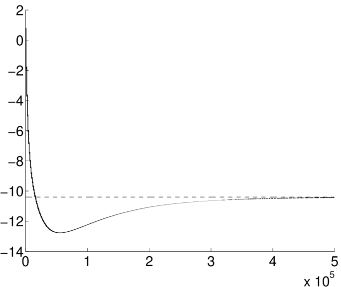
(a) $\hat{\eta}_{1}(t)$ v. t

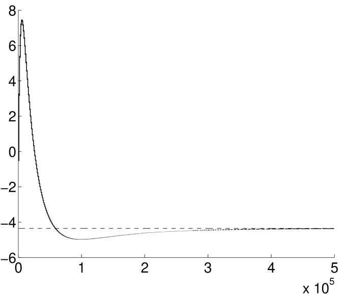
(b) $\hat{\eta}_{2}(t)$ v. t

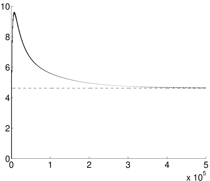
(c) $\hat{\eta}_{3}(t)$ v. t

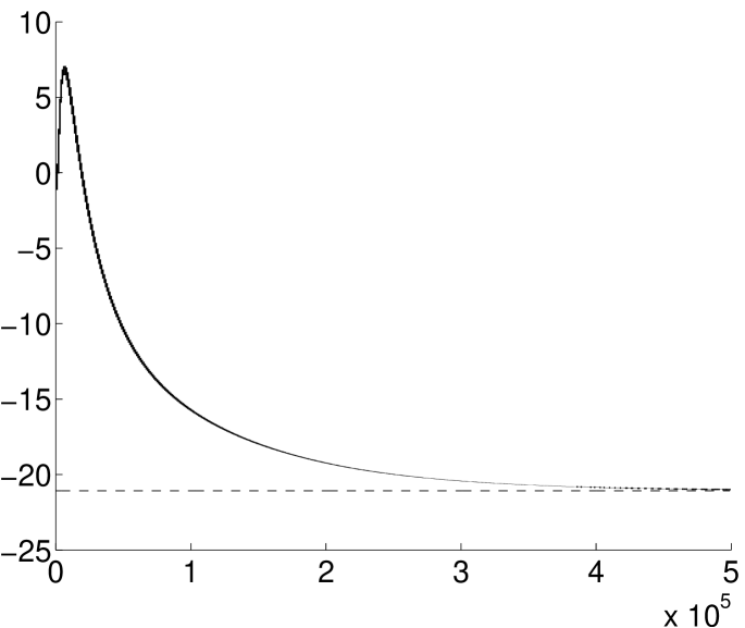
(d) $\hat{\eta}_{5}(t)$ v. t

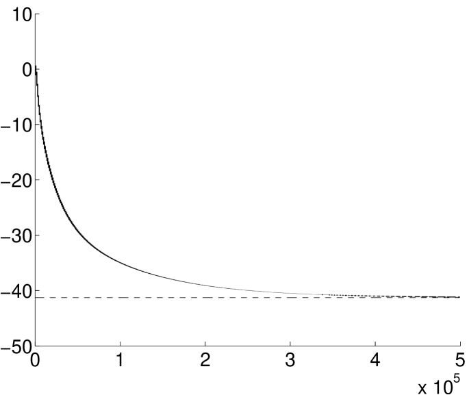
(e) $\hat{\eta}_{6}(t)$ v. t

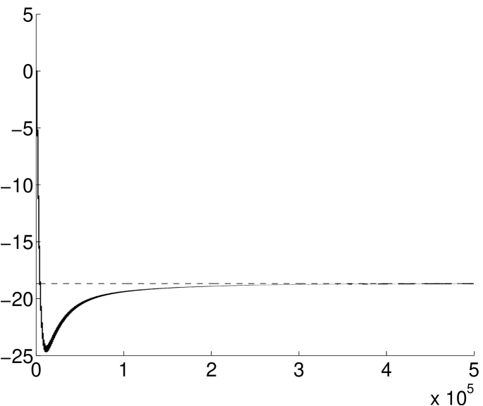
(f) $\hat{\eta}_{7}(t)$ v. t

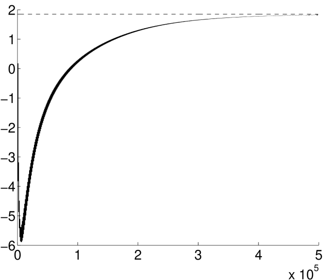
(g) $\hat{\eta}_{8}(t)$ v. t

Figure 3: Simulation results for Bastin-Gevers observer. Each $\hat{\eta}_{i}(t)$, $i\neq 4$ are shown with the true values indicated with a broken line. The periodic time of the spikes is circa $10$ seconds while the total time simulated is $5\times 10^{5}$ seconds, thus the figure spans thousands of spike cycles. The visual effect of these extreme time scales is seen in the figure; hunting oscillations within the observer are seen as thickening of the graphs of certain estimated parameters.

5.2. Parameter estimation of the 2D Hindmarsh-Rose model with Mario-Tomei observer

In addition to simulating the Bastin-Gever observer for the Hindmarsh-Rose model we also simulated observer (3.70) derived within the framework of the approach presented in [23]. In this case we set

$$\theta_{1,3}=-1,\ \theta_{1,2}=3,\ \theta_{1,3}=0,\ \theta_{1,0}=1.5,\ \theta_{2,3}=0,\ \theta_{2,2}=-5,\ \theta_{2,1}=0,\ \lambda=-1$$

There is no particular reasoning behind our choice of parameters in both this and previous case apart from that these parameters must induce persistent oscillatory dynamics of the solutions of (3.3). Parameters of the observer were chosen as follows:

$$l_{1}=l_{2}=1,\ \gamma=1,\ k=1.$$

Simulation results for this system are shown in Figure 4.

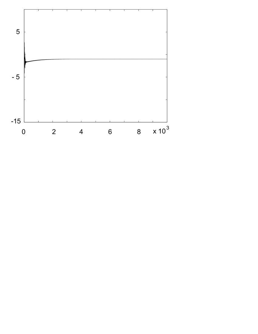
(a) $\hat{\upsilon}_{1}(t)$ v. t

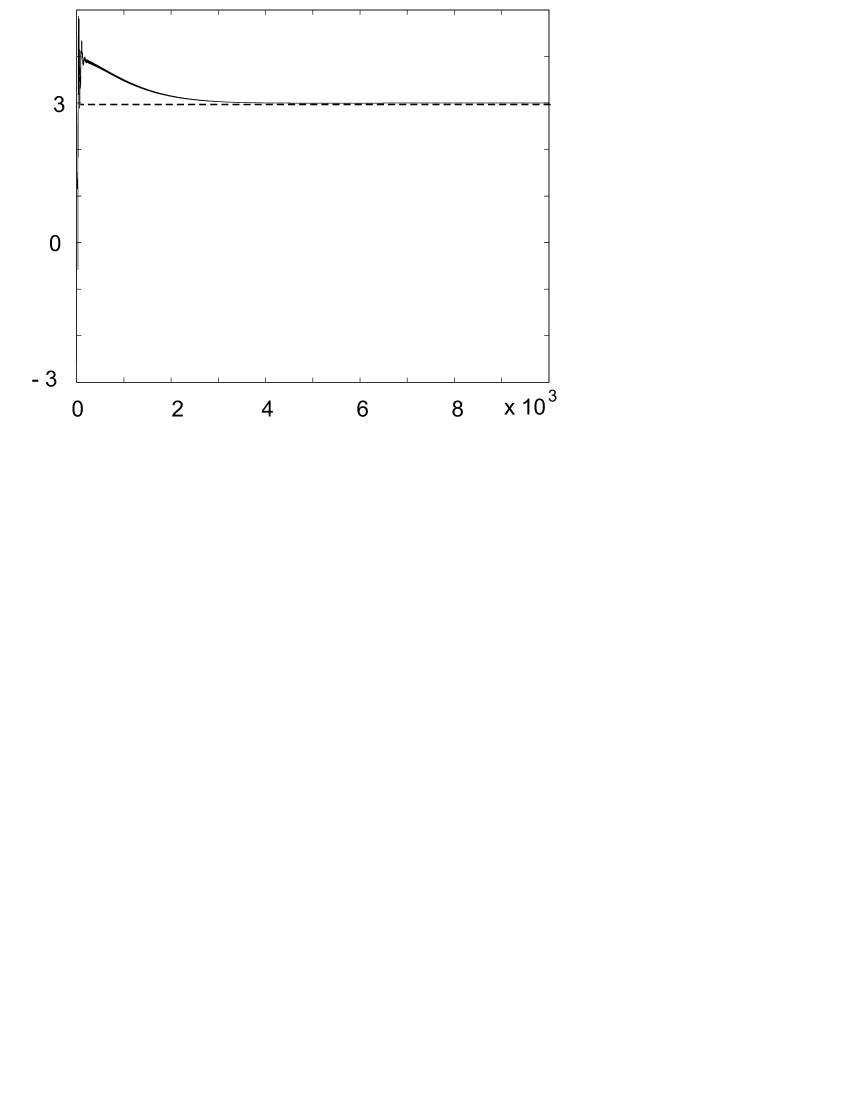
(b) $\hat{\upsilon}_{2}(t)$ v. t

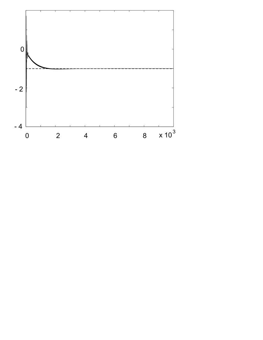
(c) $\hat{\upsilon}_{3}(t)$ v. t

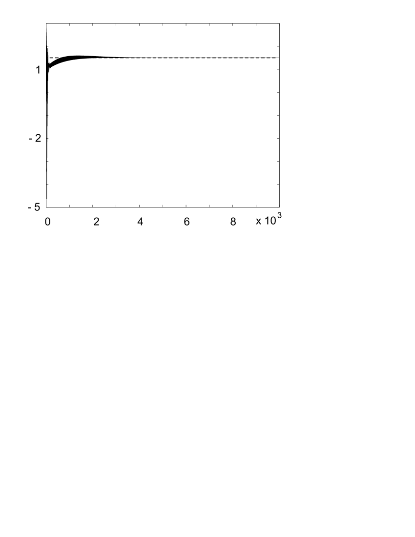
(d) $\hat{\upsilon}_{4}(t)$ v. t

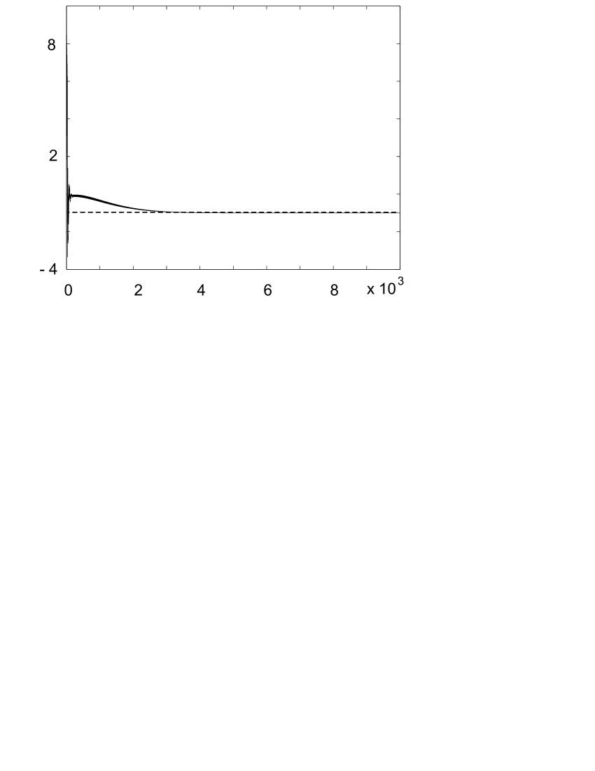
(e) $\hat{\upsilon}_{5}(t)$ v. t

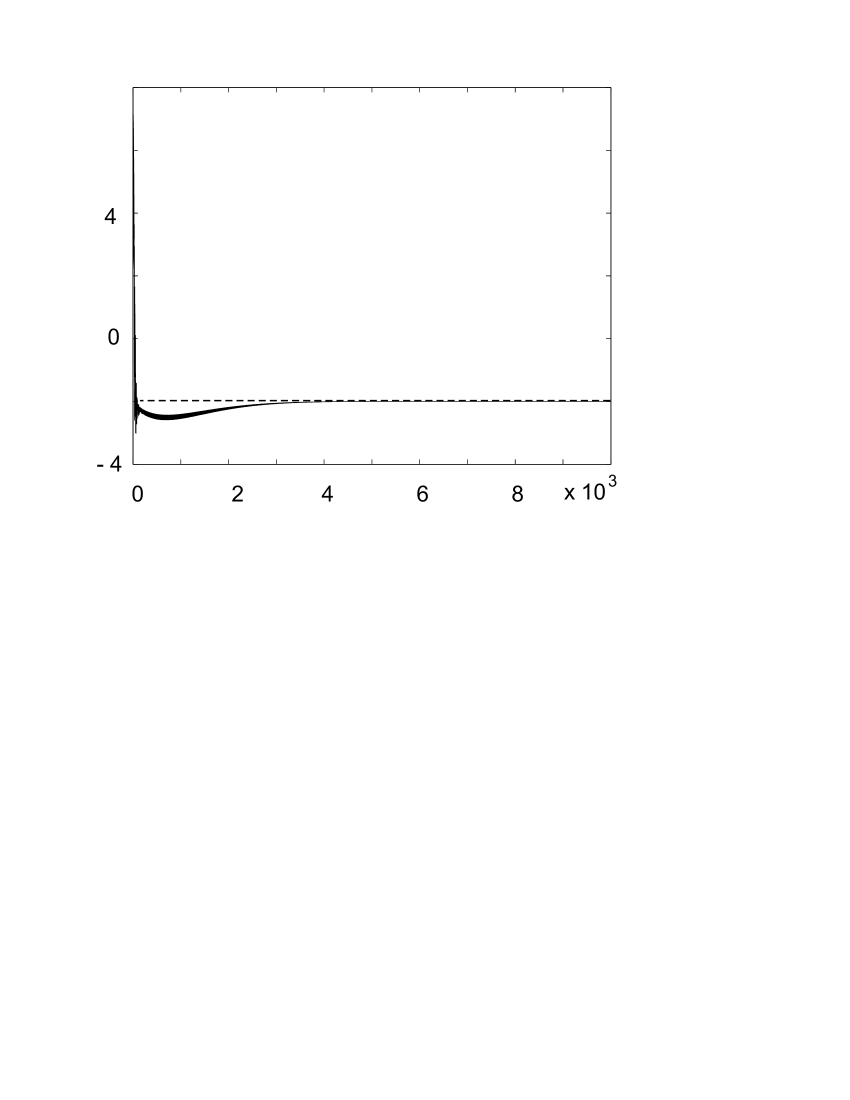
(f) $\hat{\upsilon}_{6}(t)$ v. t

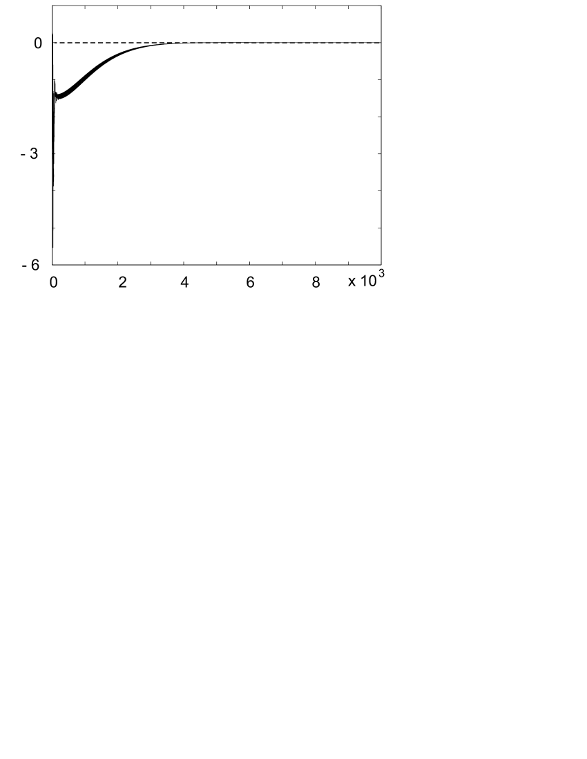
(g) $\hat{\upsilon}_{7}(t)$ v. t

Figure 4: Simulation results for Marino-Tomei observer. Each $\hat{\upsilon}_{i}(t)$ are shown with the true values indicated with a broken line. The periodic time of the spikes is circa $10$ seconds while the total time simulated is $10\times 10^{3}$ seconds, thus the figure spans thousands of spike cycles. The visual effect of these extreme time scales is seen in the figure; hunting oscillations within the observer are seen as thickening of the graphs of certain estimated parameters.

5.3. Parameter estimation of the Morris-Lecar model

Let us now turn to a more realistic class of equations, i.e. conductance-based models. In particular, we consider the Morris-Lecar model, [28]:

$$\begin{split}\dot{V}&=\frac{1}{C}\left(-\bar{g}_{\mathrm{Ca}}m_{\infty}(V)(V-E_{\mathrm{Ca}})-\bar{g}_{K}w(V-E_{K})-\bar{g}_{L}(V-V_{0})\right)+I\\ \dot{w}&=-\frac{1}{\tau(V)}w+\frac{w_{\infty}(V)}{\tau(V)}\end{split}$$ (5.1)

where

$$\begin{split}m_{\infty}(V)&=0.5\left(1+\tanh\left(\frac{V-V_{1}}{V_{2}}\right)\right)\\ w_{\infty}(V)&=0.5\left(1+\tanh\left(\frac{V-V_{3}}{V_{4}}\right)\right)\\ \tau(V)&=T_{0}\frac{1}{\cosh\left(\frac{V-V_{3}}{2V_{4}}\right)}\end{split}$$

System (5.1) is a reduction of the standard $4$-dimensional Hodgkin-Huxley equations, and is one of the simplest models describing the dynamics of evoked membrane potential and, at the same time, claiming biological plausibility.

Parameters $\bar{g}_{\mathrm{Ca}}$, $\bar{g}_{K}$, and $\bar{g}_{L}$ stand for the maximal conductances of the calcium, potassium and leakage currents respectively; $C$ is the membrane capacitance; $V_{1}$, $V_{2}$, $V_{3}$, $V_{4}$ are the parameters of the gating variables; $T_{0}$ is the parameter regulating the time scale of ionic currents; $E_{\mathrm{Ca}}$ and $E_{\mathrm{K}}$ are the Nernst potentials of the calcium and potassium currents, and $E_{L}$ is the rest potential. Variable $I$ models an external stimulation current. In this example the value of $I$ was set to $I=10$.

The total number of parameters in system (5.1) is $12$, excluding the stimulation current $I$. Some of these parameters, however, are already available or can be considered typical. For example the values of the Nernst potentials for calcium and potassium channels, $E_{\mathrm{Ca}}$, $E_{\mathrm{K}}$, are known and usually are set as follows $E_{\mathrm{Ca}}=100$, $E_{\mathrm{K}}=-70$. The value of the rest potential, $V_{0}$, can be estimated from the cell explicitly. Here we set $V_{0}=-50$. Parameters $V_{1}$, $V_{2}$ characterize the steady-state response curve of the activation gates corresponding to the calcium channels, and $V_{3}$, $V_{4}$ are the parameters of the potassium channels. In the simulations we set these parameters to standard values as e.g. in [16]: $V_{1}=-1$, $V_{2}=15$, $V_{3}=10$, and $V_{4}=29$.

The values of parameters, $\bar{g}_{\mathrm{Ca}}$, $\bar{g}_{K}$, $\bar{g}_{L}$, and $T_{0}$, however, may vary substantially from one cell to another. For example, the values of $\bar{g}_{\mathrm{Ca}}$, $\bar{g}_{K}$, $\bar{g}_{L}$ depend on the density of ion channels in a patch of the membrane; the value of $T_{0}$ is dependent on temperature. Hence, in order to model the dynamics of individual cells, we need to be able to recover these values from data.

As before, we suppose that the values of $V$ over time are available for direct observation, and the values of $w$ are not measured. System (5.1) has no linear time-invariant part, and the dynamics of $w$ are governed by a nonlinear differential equation with the time-varying relaxation factor, $1/\tau(V)$. Therefore, observers presented in Section 3 may not be applied explicitly to this system. This does not imply, however, that parameters $\bar{g}_{\mathrm{Ca}}$, $\bar{g}_{K}$, $\bar{g}_{L}$, and $T_{0}$ cannot be recovered from the measurements of $V$. In fact, as we show below, one can successfully reconstruct these parameters by using observers defined in Section 4.

For the sake of notational consistency we denote $x_{0}=V$, $x_{1}=w$, and without loss of generality suppose that $C=1$. Hence system (5.1) can now be rewritten as follows:

$$\begin{split}\dot{x}_{0}&=\theta_{0,1}m_{\infty}(x_{0})(x_{0}-E_{\mathrm{Ca}})+\theta_{0,1}x_{1}(x_{0}-E_{K})+\theta_{0,3}(x_{0}-V_{0})+I\\ \dot{x}_{1}&=-\beta_{1}(x_{0},\lambda)x_{1}+\frac{1}{\lambda}\phi_{1}(x_{0})\end{split}$$ (5.2)

where

$$\begin{split}\beta_{1}(x_{0},\lambda)&=\frac{1}{\lambda}\cosh\left(\frac{x_{0}-V_{3}}{2V_{4}}\right),\ \lambda=T_{0}\\ \phi_{1}(x_{0})&=\cosh\left(\frac{x_{0}-V_{3}}{2V_{4}}\right)w_{\infty}(x_{0})\end{split}$$

Noticing that $\beta_{1}(x_{0},\lambda)$ is separated away from zero for all bounded $x_{0}$ and positive $\lambda$ we substitute variable $x_{1}$ in (5.2) with its estimation

$$\chi(\lambda,t)=\int_{t-T}^{t}\frac{1}{\lambda}e^{-\frac{1}{\lambda}\int_{\tau}^{t}\cosh\left(\frac{x_{0}(s)-V_{3}}{2V_{4}}\right)ds}\cosh\left(\frac{x_{0}(\tau)-V_{3}}{2V_{4}}\right)w_{\infty}(x_{0}(\tau))d\tau$$

The larger the value of $T$ the higher the accuracy of estimation for large $t$. After this substitution system (5.2) reduces to just only one equation

$$\begin{split}\dot{x}_{0}&=\theta_{0,1}\phi_{0,1}(x_{0})+\theta_{0,2}\phi_{0,2}(x_{0},\lambda,t)+\theta_{0,3}\phi_{0,3}(x_{0})+I+\xi_{0}(t)\end{split}$$ (5.3)

where

$$\begin{split}\phi_{0,1}(x_{0})&=m_{\infty}(x_{0})(x_{0}-E_{\mathrm{Ca}})\\ \phi_{0,2}(x_{0},\lambda,t)&=(x_{0}-E_{K})\chi(\lambda,t)\\ \phi_{0,3}(x_{0})&=(x_{0}-V_{0})\end{split}$$

and term $\xi_{0}(t)$ is bounded.

Equation (5.3) is a special case of (4.1), and hence we can apply the results of Section 4 to construct an observer for asymptotic estimation of the values of $\theta_{0,1}$, $\theta_{0,2}$, $\theta_{0,3}$, and $\lambda$. In accordance with (4.8) – (4.10) we obtain the following observer equations

$$\begin{split}\dot{\hat{x}}_{0}&=-\alpha(\hat{x}_{0}-x_{0})+\hat{\theta}_{1}\phi_{0,1}(x_{0})+\hat{\theta}_{2}\phi_{0,2}(x_{0},\hat{\lambda},t)+\hat{\theta}_{3}\phi_{0,3}(x_{0})+I\\ \dot{\hat{\theta}}_{1}&=-\gamma_{\theta}(\hat{x}_{0}-x_{0})\phi_{0,1}(x_{0})\\ \dot{\hat{\theta}}_{2}&=-\gamma_{\theta}(\hat{x}_{0}-x_{0})\phi_{0,2}(x_{0},\hat{\lambda},t)\\ \dot{\hat{\theta}}_{3}&=-\gamma_{\theta}(\hat{x}_{0}-x_{0})\phi_{0,3}(x_{0})\end{split}$$ (5.4)

$$\begin{split}\hat{\lambda}&=3+\hat{x}_{1,1}\\ \dot{\hat{x}}_{1,1}&=\gamma e\left(\hat{x}_{1,1}-\hat{x}_{2,1}-\hat{x}_{1,1}\left(\hat{x}_{1,1}^{2}+\hat{x}_{2,1}^{2}\right)\right)\\ \dot{\hat{x}}_{2,1}&=\gamma e\left(\hat{x}_{1,1}+\hat{x}_{2,1}-\hat{x}_{2,1}\left(\hat{x}_{1,1}^{2}+\hat{x}_{2,1}^{2}\right)\right)\\ e&=\sigma(\|x_{0}-\hat{x}_{0}\|_{\varepsilon})\end{split}$$ (5.5)

Parameters of the observer were set as follows: $\alpha=1$, $\varepsilon=0.001$, $\gamma=0.01$, $\gamma_{\theta}=0.05$.

According to Theorems 15, 17 observer (5.4), (5.5) should ensure successful reconstruction of the model parameters provided that the regressor is persistently exciting. This requirement is satisfied for model (5.2) generating periodic solutions. We simulated system (5.2), (5.4), (5.5) over a wide range of initial conditions. Figure 5 shows an example of typical behavior of the observer over time. As we can see from this figure all estimates converge to small neighborhoods of true values of the parameters.

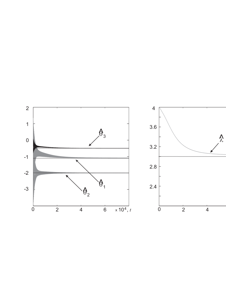
Figure 5: Trajectories of the estimates of parameters $\theta_{1}$, $\theta_{2}$, $\theta_{3}$ and $\lambda$ as functions of time. The periodic time of the spikes is circa $10$ seconds while the total time simulated is $8\times 10^{4}$ seconds, thus the figure spans thousands of spike cycles. The visual effect of these extreme time scales is seen in the figure; hunting oscillations within the observer are seen as thickening of the graphs of certain estimated parameters.

6. Conclusion

In this article we have reviewed and explored observer-based approaches to the problem of state and parameter reconstruction for classes of typical models of neural oscillators. The estimation procedure in this approach is defined as a system of ordinary differential equations of which the right-hand side does not depend explicitly on the unmeasured variables. The solution of this system (or functions of the solutions) should asymptotically converge to small neighbourhoods of the actual values of the variables to be estimated. Until recently, due to nonlinear dependence of the vector-fields of the models on unknown parameters and also due to uncertainties in the time scales of hidden variables, observer-based approach to solving the problem of state and parameter estimation of neural oscillators was a relatively unexplored territory. Here we demonstrate that despite these obvious difficulties the approach can be successfully applied to a wide range of models.

Two different strategies to observer design have been studied in the paper. The first strategy is based on the availability of canonical representations of the original system. Success of this strategy is obviously determined by wether one can find a suitable coordinate transformation such that the equations of the original model can be transformed into the canonical adaptive observer form. Because a coordinate transformation is required, different classes of models are likely to lead to different observers. The second strategy is based on the ideas and approaches of universal adaptive regulation [11], non-uniform convergence and non-uniform small-gain theorems [35], [36]. The structure of observers obtained as a result of this design strategy does not change much from one model to another. The main difference between these design strategies is in the convergence rates: exponential for the first and asymptotical for the second. As long as mere overall convergence time is accounted for there is no big difference whether the convergence itself is exponential or not. Yet, the fact that it can be made exponential with known rates of convergence allows us to derive the a-priori estimates of the amount of time needed to achieve a certain given accuracy of estimation.

We have shown that for linearly parameterized models such as the FitzHugh-Nagumo and Hindmarsh-Rose oscillators one can develop an observer for state and parameter estimation of which the convergence rate is exponential. For the nonlinearly parameterized and more realistic models such as the Morris-Lecar and Hodgkin-Huxley equations we presented an observer of which the convergence is asymptotic. In both cases the rate of convergence depends on the degree of excitation in the measured data. In the case of linearly parameterized systems this excitation can be measured by the minimal eigenvalue of a certain matrix constructed explicitly from the data and the model. For the nonlinearly parameterized systems the degree of excitation is defined by a more complex expression, (4.14). In principle, one can ensure arbitrarily fast convergence of the estimator provided that the excitation is sufficiently high. This property motivates the development of measurements protocols that are most consistent with a range of models that will be fitted to the collected data. In fact, in order to achieve higher computational effectiveness, one shall aim to produce data of which the excitation is higher for the given range of models.

One question remains unexplored though – the actual amount of elementary computational operations required to realize these two observer schemes. This number depends substantially on the required accuracy of estimation. We aim to answer this important question in future case studies.

7. Appendix

Proof of Theorem 6

Proof.

The proof is straightforward. Indeed, for the observability test we have

$$\left(\begin{array}[]{c}h(x)\\ L_{f}h(x)\\ L^{2}_{f}h(x)\\ .\\ .\\ .\\ L^{n-1}_{f}h(x)\end{array}\right)=\left(\begin{array}[]{c}x_{1}\\ x_{2}+x_{3}+...+x_{n}\\ 0\\ .\\ 0\end{array}\right)$$ (7.13)

and

$$\frac{\partial}{\partial x}\left(\begin{array}[]{c}h(x)\\ L_{f}h(x)\\ L^{2}_{f}h(x)\\ .\\ .\\ .\\ L^{n-1}_{f}h(x)\end{array}\right)=\left(\begin{array}[]{ccccccc}1&0&0&0&0&...&0\\ 0&1&1&1&1&...&1\\ 0&0&0&0&0&...&0\\ .&.&.&.&.&...&.\\ 0&0&0&0&0&...&0\end{array}\right)$$ (7.26)

It follows that observability is lost for $n>2$. This proves condition (i). In order to demonstrate condition (ii) we use theorem 5 as follows. From equation (2.72) we have

$$\left\langle\left(\begin{array}[]{cc}1&0\\ 0&1\end{array}\right),\left(\begin{array}[]{c}g_{1}\\ g_{2}\end{array}\right)\right\rangle=\left(\begin{array}[]{c}0\\ 1\end{array}\right)$$ (7.33)

giving

$$g=\left(\begin{array}[]{c}0\\ 1\end{array}\right)$$ (7.36)

Theorem 5 condition (i) will be satisfied since the system is linear and from theorem 5 part (ii) we have

$$[q_{1},ad^{0}_{f}g] = [q_{1},g]$$ (7.37)

$$= \frac{\partial g}{\partial x}q_{1}-\frac{\partial q_{1}}{\partial x}g$$ (7.38)

$$= -\frac{\partial q_{1}}{\partial x}\left(\begin{array}[]{c}0\\ 1\end{array}\right)$$ (7.41)

$$= -\frac{\partial q_{1}}{\partial x_{2}}$$ (7.42)

we satisfy theorem 5 part (ii) if and only if $\partial{q_{1}}/{\partial x_{2}}=\mathbf{0}$ for all $x\in U$. ∎

Proof of Corollary 8

Proof.

The proof of the corollary is straightforward. Consider the error system given by (3.67). Given that the function $\varphi(t)$ is bounded one can easily see that $\hat{\eta}$, $\hat{x}$ are bounded as well (consider e.g. the following Lyapunov candidate: $V=\|\tilde{x}^{\ast}\|^{2}+\tilde{\eta}\Gamma^{-1}\tilde{\eta}$). This implies that component $\varphi_{4}(t)\tilde{\eta}_{4}(t)$ is converging to zero exponentially.

Let us denote

$$\bar{\eta}=(\tilde{\eta}_{1},\tilde{\eta}_{2},\tilde{\eta}_{3},\tilde{\eta}_{5},\tilde{\eta}_{6},\tilde{\eta}_{7},\tilde{\eta}_{8})^{T}$$

and consider the following reduced error dynamics

$$\begin{array}[]{c}\dot{\tilde{x}}^{*}=\left(\begin{array}[]{cc}-c_{1}&k\\ 0&f\end{array}\right)\tilde{x}^{*}+\left(\begin{array}[]{c}\bar{\varphi}^{T}\bar{\eta}\\ 0\end{array}\right)+p\varepsilon(t)\\ \dot{\bar{\eta}}=-\Gamma\bar{\varphi}\tilde{x}_{1}^{*}\end{array}$$ (7.49)

in which $\varepsilon(t)$ stands for the term $\varphi_{4}(t)\tilde{\eta}_{4}(t)$, and $p=(1,0)^{T}$. System (7.49) is a linear time-varying system of which the homogenous part is exponentially stable provided that $\bar{\varphi}(t)$ is persistently exciting (this follows explicitly from Theorem 4). Hence, taking into account that $\varepsilon(t)$ is an exponentially converging to zero term, we can conclude that $\tilde{x}^{\ast}$, $\bar{\eta}$ converge to the origin too and that such convergence is exponential. ∎

Proof of Theorem 10

Proof.

The proof of the theorem is standard and can be constructed from many other more general results (see for example [23], [29]). Here we present just a sketch of the argument for consistency. According to our assumptions, matrix $A_{1}+LC_{1}$ is Hurwitz. Moreover, the transfer function

$$H(s)=C_{1}(s-(A_{1}+LC_{1}))^{-1}b=\frac{s+k}{s^{2}+(k+1)s+k}=\frac{s+k}{(s+k)(s+1)}$$

is strictly positive real. Hence, using the Kalman-Yakubovich-Popov lemma, we can conclude that there exists a symmetric and positive definite matrix $H$ such that

$$H(A_{1}+LC_{1})+(A_{1}+LC_{1})^{T}H<-Q,\ Hb=(1,0)^{T},$$ (7.50)

where $Q$ is a positive definite matrix. Let us now consider the following function

$$V(z,\hat{\upsilon},t)=\frac{1}{2}(z-\hat{z})^{T}H(z-\hat{z})+\frac{1}{2}\|\upsilon-\hat{\upsilon}\|^{2}\gamma^{-1}+D\int_{t}^{\infty}\varepsilon^{2}(\tau)d\tau$$

where the value of $D$ is to be specified later. Clearly, the function $V$ is well-defined for the term $\varepsilon(t)$ is continuous and exponentially decaying to zero as $t\rightarrow\infty$. Thus the boundedness of $V$ implies that $\|\hat{z}-z\|$ and $\|\hat{\upsilon}-\upsilon\|$ are bounded.

Consider the time-derivative of $V$:

$$\begin{split}\dot{V}&=(z-\hat{z})^{T}(H(A_{1}+LC_{1})+(A_{1}+LC_{1})^{T}H)(z-\hat{z})+(z-\hat{z})^{T}Hb\phi^{T}(z_{1},t)(\upsilon-\hat{\upsilon})\\ &+(z-\hat{z})^{T}Hb\varepsilon-(\upsilon-\hat{\upsilon})(1,0)(z-\hat{z})\phi(z_{1},t)-D\varepsilon^{2}\end{split}$$

Taking (7.50) into account we obtain:

$$\begin{split}\dot{V}&\leq-(z-\hat{z})^{T}Q(z-\hat{z})+\|z-\hat{z}\||\varepsilon(t)|M-D\varepsilon^{2}\leq-\alpha\|z-\hat{z}\|^{2}+\\ &\|z-\hat{z}\||\varepsilon(t)|M-D\varepsilon^{2},\end{split}$$ (7.51)

where $\alpha>0$ is the minimal eigenvalue of $Q$, $M$ is fixed positive number, and $D$ is a parameter of $V$ which can be chosen arbitrarily and independently of $M$. Choosing $D$ such that

$$\sqrt{\frac{\alpha D}{4}}=M,$$

we ensure that

$$\dot{V}\leq-\frac{\alpha}{2}\|z-\hat{z}\|^{2}$$

Thus the function $V$ is bounded from above, and given that the solution $z(t)$ exists for all $t>t_{0}$ so does the solution of the combined system. The rest of the proof follows directly from Barbalatt’s lemma and the asymptotic stability theorem for the class of skew-symmetric time-varying systems presented in [27]. ∎

References

• [1] H.D.I. Abarbanel, D.R. Crevling, R. Farsian and M. Kostuk. Dynamical State and Parameter Estimation. SIAM J. Applied Dynamical Systems, 8(4):1341–1381, 2009.
• [2] P. Achard and E. Schutter. Complex parameter landscape for a comples neuron model. PLOS Computational Biology, 2(7):794–804, 2006.
• [3] G. Bastin and M. Gevers. Stable adaptive observers for nonlinear time-varying systems. IEEE Trans. on Automatic Control, 33(7):650–658, 1988.
• [4] R. Borisyuk and Y. Kazanovich. Oscillations and waves in the models of interactive neural populations. Biosystems, 86(1–3):53–62, 2006.
• [5] D. Brewer, M. Barenco, R. Callard, M. Hubank, and J. Stark. Fitting ordinary differential equations to short time course data. Philosophical Transactions of The Royal Society A, 366(1865):519–544, 2008.
• [6] C. Cao, A.M. Annaswamy, and A. Kojic. Parameter convergence in nonlinearly parametrized systems. IEEE Trans. on Automatic Control, 48(3):397–411, 2003.
• [7] R. FitzHugh. Impulses and physiological states in theoretical models of nerve membrane. Biophysical Journal, 1:445–466, 1961.
• [8] A.N. Gorban. Basic types of coarse-graining. In A.N. Gorban, N. Kazantzis, I.G. Kevrekidis, H.C. Ottinger, and C. Theodoropoulos, editors, Model Reduction and Coarse–Graining Approaches for Multiscale Phenomena, pages 117–176. Springer, 2006.
• [9] J.L. Hindmarsh and R.M. Rose. A model of neuronal bursting using three coupled first order differential equations. Proc. R. Soc. Lond., B 221(1222):87–102, 1984.
• [10] A.L. Hodgkin and A.F. Huxley. A quantitative description of membrane current and its application to conduction and excitation in nerve. J. Physiol., 117:500–544, 1952.
• [11] A. Ilchman. Universal adaptive stabilization of nonlinear systems. Dyn. and Contr., (7):199–213, 1997.
• [12] A. Isidori. Nonlinear control systems II. Springer–Verlag, second edition, 1999.
• [13] E. M. Izhikevich. Dynamical Systems in Neuroscience: the Geometry of Excitability and Bursting. MIT Press, 2007.
• [14] E. M. Izhikevich and G. M. Edelman. Large-scale model of mammalian thalamocortical systems. Proc. of Nat. Acad. Sci., 105:3593–3598, 2008.
• [15] Y. Kazanovich and R. Borisyuk. An oscillatory neural model of multiple object tracking. Neural Computation, 18(6):1413–1440, 2006.
• [16] C. Koch. Biophysics of Computation. Information Processing in Signle Neurons. Oxford University Press, 2002.
• [17] G. Kreisselmeier. Adaptive obsevers with exponential rate of convergence. IEEE Trans. Automatic Control, AC-22:2–8, 1977.
• [18] W. Lin and C. Qian. Adaptive control of nonlinearly parameterized systems: The smooth feedback case. IEEE Trans. Automatic Control, 47(8):1249–1266, 2002.
• [19] L. Ljung. System Identification: Theory for the User. Prentice-Hall, 1999.
• [20] L. Ljung. Perspectives in system identification. In Proceedings of the 17-th IFAC World Congress on Automatic Control, pages 7172–7184. 2008.
• [21] A. Loria and E. Panteley. Uniform exponential stability of linear time-varying systems: revisited. Systems and Control Letters, 47(1):13–24, 2003.
• [22] A.M. Lyapunov. The general problem of the stability of motion. Int. Journal of Control, 55(3), 1992.
• [23] R. Marino. Adaptive observers for single output nonlinear systems. IEEE Trans. Automatic Control, 35(9):1054–1058, 1990.
• [24] R. Marino and P. Tomei. Global adaptive observers for nonlinear systems via filtered transformations. IEEE Trans. Automatic Control, 37(8):1239–1245, 1992.
• [25] R. Marino and P. Tomei. Adaptive observers with arbitrary exponential rate of convergence for nonlinear systems. IEEE Trans. Automatic Control, 40(7):1300–1304, 1995.
• [26] J. Milnor. On the concept of attractor. Commun. Math. Phys., 99:177–195, 1985.
• [27] A. P. Morgan and K. S. Narendra. On the stability of nonautonomous differential equations $\dot{x}=[{A}+{B}(t)]x$ with skew symmetric matrix ${B}(t)$. SIAM J. Control and Optimization, 37(9):1343–1354, 1977.
• [28] C. Morris and H. Lecar. Voltage oscillatins in the barnacle giant muscle fiber. Biophysics J., 35:193–213, 1981.
• [29] K. S. Narendra and A. M. Annaswamy. Stable Adaptive systems. Prentice–Hall, 1989.
• [30] H. Nijmeijer and A. van der Schaft. Nonlinear Dynamical Control Systems. Springer–Verlag, 1990.
• [31] A. Prinz, C.P. Billimoria, and E. Marder. Alternative to hand-tuning conductance-based models: Contruction and analysis of databases of model neurons. Journal of Neorophysiology, 90:3998–4015, 2003.
• [32] I. Yu. Tyukin, D.V. Prokhorov, and C. van Leeuwen. Adaptive algorithms in finite form for nonconvex parameterized systems with low-triangular structure. In Proceedings of the 8-th IFAC Workshop on Adaptation and Learning in Control and Signal Processing (ALCOSP 2004), pages 261–266. 2004.
• [33] I.Yu. Tyukin, D. V. Prokhorov, and C. van Leeuwen. Adaptation and parameter estimation in systems with unstable target dynamics and nonlinear parametrization. IEEE Transactions on Automatic Control, 52(9):1543 – 1559, 2007.
• [34] I.Yu. Tyukin, D.V. Prokhorov, and V.A. Terekhov. Adaptive control with nonconvex parameterization. IEEE Trans. on Automatic Control, 48(4):554–567, 2003.
• [35] I.Yu. Tyukin, E. Steur, H. Nijmeijer, and C. van Leeuwen. Non-uniform small-gain theorems for systems with unstable invariant sets. SIAM Journal on Control and Optimization, 47(2):849–882, 2008.
• [36] I.Yu. Tyukin, E. Steur, H. Nijmeijer, and C. van Leeuwen. Adaptive observers and parametric identification for systems in non-canonical adaptive observer form. Submitted, preprint available at http://arxiv.org/abs/0903.2361, 2009.
• [37] W. van Geit, E. de Shutter, and P. Achard. Automated neuron model optimization techniques: a review. Biol. Cybern, 99:241–251, 2008.
• [38] Kazantsev V.B., Nekorkin V.I., Makarenko V.I., and Llinas R. Self-referential phase reset based on inferior olive oscillator dynamics. Proceedings of National Academy of Science, 101(52):18183–18188, 2004.