Glass transition and random walks on complex energy landscapes

Abstract

We present a simple mathematical model of glassy dynamics seen as a random walk in a directed, weighted network of minima taken as a representation of the energy landscape. Our approach gives a broader perspective to previous studies focusing on particular examples of energy landscapes obtained by sampling energy minima and saddles of small systems. We point out how the relation between the energies of the minima and their number of neighbors should be studied in connection with the network’s global topology, and show how the tools developed in complex network theory can be put to use in this context.

The physics of glassy systems, the glass transition, and the slow dynamics ensuing at low temperatures have been the subject of a large interest in the past decades Debenedetti . In particular, special attention has been devoted to the dynamics of a glassy system inside its configuration space: The idea is to understand glassy dynamics in terms of the exploration of a complex, rugged energy landscape in which the large number of metastable states limits the ability of the system to equilibrate. In the picture of an energy landscape partitioned into basins of attraction of local minima (“traps”), the dynamics of the system is separated into harmonic vibrations inside traps and jumps between minima Angelani:1998 . Several models of dynamical evolution through jumps between traps have been proposed and studied in order to reproduce the phenomenology of the glass transition, pointing out various ingredients of the ensuing slow dynamics Bouchaud:1992 ; Monthus:1996 . Moreover, several works have mapped the energy landscape of small systems and studied the dynamics through a master equation for the time evolution of the probability to be in each minimum. Systems thus considered range from clusters of Lennard-Jones atoms to proteins or heteropolymers Angelani:1998 ; Cieplak:1998 ; Bongini:2008b ; Carmi:2009 .

The success of these approaches has recently brought about a number of studies focusing on the topology of the network defined by considering the minima as nodes and the possibility of a jump between two minima as a (weighted, directed) link newman-review . The small-world character of these networks has been pointed out Scala:2001 , as well as strong heterogeneity in the number of links of each node (its degree). Scale-free distributions have been observed Doye:2002 , and linked to scale-free distributions of the areas of the basins of attraction Massen:2005 ; Seyed:2008 . Further investigations of various energy landscapes (of Lennard-Jones atoms, proteins, spin glasses) have used complex network analysis tools Doye:2005 ; Bongini:2008b ; Seyed:2008 ; Carmi:2009 ; network_as_a_tool . For instance, some works have exposed a logarithmic dependence of the energy of a minimum on its degree Doye:2002 ; Seyed:2008 ; Carmi:2009 , or energy barriers increasing as a (small) power of the degree of a node Carmi:2009 . However, the relation between the energy and the degree of a minimum has never been systematically investigated. Moreover, no systematic study of the connection between the network of minima and the glassy dynamics has been performed, since the studies cited above are limited to small size systems.

Here, we make an important first step to fill this gap by putting forward a simple mathematical model of a network of minima, through a generalization of Bouchaud’s trap model Bouchaud:1992 ; Monthus:1996 . This framework allows to use the wide body of knowledge developed recently on dynamical phenomena in complex networks Barrat:2008 to study the dynamics in a complex energy landscape as a random walk in a directed, weighted complex network. The corresponding heterogeneous mean-field (HMF) theory DorogoRev highlights the connection between network properties and dynamics, and shows in particular that the relationship between energy and degree of the minima is a crucial ingredient for the existence of a transition and the subsequent glassy phenomenology. This approach sheds light on the fact that scale-free structures and logarithmic relations between degrees and energies have been empirically found, and should stimulate more systematic investigations on this issue. It also puts previous studies of the dynamics in a network of minima obtained empirically in a broader perspective.

We consider the well-known traps model of phase space consisting in $N$ traps, $i=1,\cdots,N$, of random depths $E_{i}$ extracted from a distribution $\rho(E)$ Bouchaud:1992 ; Monthus:1996 . The dynamics is given by random jumps between traps: The system, at temperature $T=1/\beta$, remains in a trap for a time $\tau_{0}\exp(\beta E)$ (where $\tau_{0}$ is a microscopic timescale that we can set equal to $1$), and then jumps to a new, randomly chosen trap; all traps are connected to each other, in a fully connected topology. Here we consider instead a—more realistic—case in which the traps form a network: Each trap $i$ has depth $E_{i}$ and number of neighbors $k_{i}$. The system, pictured as a random walker in this network, escapes from a trap of depth $E_{i}$ towards one of the $k_{i}$ neighboring traps of depth $E_{j}$ with a rate $r_{i\to j}$, which is a priori a function of both $E_{i}$ and $E_{j}$. Possible rates include Metropolis $\frac{1}{k_{i}}\min\left(1,e^{\beta(E_{j}-E_{i})}\right)$ or Glauber $k_{i}^{-1}/\left(1+e^{-\beta(E_{j}-E_{i})}\right)$ ones. For simplicity, we will stick here to the original definition of rates depending only on the initial trap, i.e. $r_{i\to j}=e^{-\beta E_{i}}/k_{i}$.

In the fully connected trap model, all traps are equiprobable after a jump, so that the probability for the system to be in a trap of depth $E$ is simply $\rho(E)$, and the average time spent in a trap is $\langle\tau\rangle=\int\rho(E)e^{\beta E}dE$. Thus, a transition occurs between a high temperature phase in which $\langle\tau\rangle$ is finite and a low temperature phase with diverging $\langle\tau\rangle$ if and only if $\rho(E)$ is of the form $\sim\exp(-\beta_{0}E)$ at large $E$ (else the transition temperature is either $0$ or $\infty$) Monthus:1996 ; the distribution of trapping times is then $P(\tau)\sim\tau^{-1-T/T_{0}}$. Let us see how this translates when the network of minima is not fully connected. In this case, it is convenient to divide the nodes in degree classes, as it is usual in the framework of the HMF theory DorogoRev . We further assume that the depth of a minimum and its degree are related: $E_{i}=f(k_{i})$ where the function $f(k)$ does not depend on $i$ and is a characteristic of the model. The time spent in a trap of degree $k$ is then $\tau_{k}=e^{\beta f(k)}$, and the transition rate $r_{i\to j}$ between two traps can be written as a function of the endpoints’ degrees $k_{i}$ and $k_{j}$. It is important to recall that, in the steady state, the probability for a random walker to find itself on a node of degree $k$ is $kP(k)/\langle k\rangle$, where $P(k)$ is the degree distribution of the network and $\langle k\rangle$ is the average degree Redner:2001 . The average rest time before a hop is therefore

$$\langle\tau\rangle=\langle k\rangle^{-1}\sum_{k}kP(k)e^{\beta f(k)}\ .$$ (1)

It is then clear that the presence of a finite transition temperature at which $\langle\tau\rangle$ becomes infinite results from an interplay between the topology of the underlying network and the relation between traps’ depth and degree. For instance, for a scale free distribution $P(k)\sim k^{-\gamma}$, a finite transition temperature is obtained if and only if $f(k)$ is of the form $E_{0}\log(k)$: $\langle\tau\rangle$ is then finite (in an infinite system) for $T>T_{c}\equiv E_{0}/(\gamma-2)$, and infinite for $T\leq T_{c}$. For $P(k)$ behaving instead as $e^{-ak^{\alpha}}$, $f(k)$ has to be of the form $E_{0}k^{\alpha}$ for a transition to occur. Thus, although important, the study of the topology of the network of minima is not enough to understand the dynamical properties of the system, and more attention should be paid to the energy/connectivity relation.

To gain further insight into the dynamics of the system we can write, within the HMF approach, the rate equation for the probability $\rho_{k}(t)$ that a given vertex of degree $k$ hosts the random walker at physical time $t$. Since the walker escapes a trap with rate per unit time $r_{k}=1/\tau_{k}$, we have

$$\frac{\partial\rho_{k}(t)}{\partial t}=-r_{k}\rho_{k}(t)+k\sum_{k^{\prime}}P(k^{\prime}|k)r(k^{\prime}\to k)\rho_{k^{\prime}}(t)$$ (2)

where $P(k^{\prime}|k)$ is the conditional probability that a random neighbor of a node of degree $k$ has degree $k^{\prime}$ newman-review . In the steady state, $\partial_{t}\rho_{k}(t)=0$, the solution of Eq. (2) for any correlation pattern $P(k^{\prime}|k)$ is Redner:2001

$$r_{k}\rho_{k}\sim k\ ,$$ (3)

and the normalized equilibrium distribution reads

$$\rho_{k}^{eq}=\frac{k\tau_{k}}{N\langle k\tau_{k}\rangle}.$$ (4)

Note that the probability for the random walker to be in any vertex of degree $k$ is then $P_{eq}(k)=NP(k)\rho_{k}^{eq}$. Since $\langle k\tau_{k}\rangle=\sum_{k}kP(k)e^{\beta f(k)}$, the conclusion is the same as before: A normalizable equilibrium distribution exists indeed if and only if $\langle k\tau_{k}\rangle<\infty$, and the presence of a transition at a finite temperature $T_{c}$ is determined by the interplay between $P(k)$ and $f(k)$.

In any finite system, the distribution $P_{eq}(k)$ exists, and the probability that the random walker is in a node of degree $k$ at time $t_{w}$, $P(k;t_{w})=NP(k)\rho_{k}(t_{w})$, converges to $P_{eq}(k)$ after a certain equilibration time. It is interesting to study this evolution in the low temperature regime, when it exists. Let us consider the case of a scale-free network with $P(k)\sim k^{-\gamma}$ newman-review and $f(k)=E_{0}\log(k)$, i.e., $\tau_{k}=k^{\beta E_{0}}$. In numerical experiments, the walker explores an underlying network generated according to the Uncorrelated Configuration Model Catanzaro:2005 , and spends in each node of degree $k$ an amount of time extracted from the distribution $P(\tau_{k})=\exp(-t/\tau_{k})/\tau_{k}$. Figure 1 shows how $P(k;t_{w})$ evolves from the distribution $kP(k)/\langle{k}\rangle$ at short times, corresponding to the degree distribution of a node reached after a random jump, to $P_{eq}(k)\sim k^{1+\beta E_{0}-\gamma}$ (obtained from Eq. (4)) at long times: The small degree region equilibrates first, and a progressive equilibration of larger and larger degree regions takes place at larger times. Small degrees correspond in fact to shallow minima, which take less time to explore, while large degree nodes are deep traps which take longer to equilibrate . At time $t_{w}$, one can therefore consider that the nodes of degree smaller than a certain $k_{w}$ are “at equilibrium”, while the larger nodes are not. Considering that the total time $t_{w}$ is the sum of the trapping times of the visited nodes, which is dominated by the longest one $k_{w}^{\beta E_{0}}$, we obtain $k_{w}\sim t_{w}^{1/(\beta E_{0})}$ . Figure 1 shows indeed that the whole non-equilibrium distribution can be cast into the scaling form

$$P(k;t_{w})=t_{w}^{-1/(\beta E_{0})}F\left(k/t_{w}^{1/(\beta E_{0})}\right)$$ (5)

where $F$ is a scaling function such that $F(x)\sim x^{1+\beta E_{0}-\gamma}$ at small $x$ and $F(x)\sim x^{1-\gamma}$ at large $x$. This evolution takes place until the largest nodes, of degree $k_{c}$, equilibrate. For an uncorrelated scale-free network, $k_{c}\sim N^{1/2}$ so that the equilibration time is $t_{eq}\sim k_{c}^{\beta E_{0}}\sim N^{\beta E_{0}/2}$.

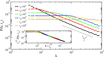
Figure 1: Evolution of $P(k;t_{w})$ for an uncorrelated scale-free network. Here $N=10^{6}$ ($k_{c}=10^{3}$), $\gamma=3$, $\beta E_{0}=2$ so that $P(k;t_{w})\sim k^{-2}$ at short times and $P_{eq}(k)\sim k^{0}$. Inset: $t_{w}^{1/2}P(k;t_{w})$ vs $k/t_{w}^{1/2}$ for $t_{w}<t_{eq}\sim 10^{6}$.

The evolution of $P(k;t_{w})$ at low temperature corresponds to the aging dynamics of the system, which is exploring deeper and deeper traps. This dynamics is also customarily investigated through a two-time correlation function $C(t_{w}+t,t_{w})$ between the states of the system at times $t_{w}$ and $t_{w}+t$, defined as the the average probability that a particle has not changed trap between $t_{w}$ and $t_{w}+t$ Bouchaud:1992 ; Monthus:1996 : this amounts to considering that the correlation is $1$ within one trap and $0$ between distinct traps. The probability that a walker remains in trap $i$ a time larger than $t$ is simply given by $\exp(-t/\tau_{i})$, so that

$$C(t_{w}+t,t_{w})=\int dk\;P(k;t_{w})e^{-t/\tau_{k}},$$ (6)

where we have used the continuous degree approximation, replacing discrete sums over $k$ by integrals. For scale-free networks, using the scaling form (5), it is then straightforward to obtain that the correlation function obeys the so-called “simple” aging $C(t_{w}+t,t_{w})=g(t/t_{w})$, as in the original trap model Monthus:1996 (Fig. 2).

Aging properties of the system can be measured also through the average time $t_{esc}(t_{w})$ required by the random walker to escape from the node it occupies at time $t_{w}$. In other words we define $t_{esc}=\langle{t^{\prime}}\rangle-t_{w}$, where $t^{\prime}>t_{w}$ is the time of the first jump performed by the walker after $t_{w}$, which gives $t_{esc}(t_{w})=\int dk\;\tau_{k}P(k;t_{w})$. For small $t_{w}$ with respect to the equilibration time, $t_{esc}$ is growing due to the evolution of $P(k;t_{w})$. At long enough times, in any finite system, $\rho_{k}(t_{w})\to\rho_{k}^{eq}$ so that

$$t_{esc}(t_{w}\to\infty)=\int dk\;\frac{kP(k)e^{2\beta f(k)}}{\langle k\tau_{k}\rangle}.$$ (7)

Interestingly, this formula shows that, whenever $P(k)$ and $f(k)$ are such that a finite transition temperature $T_{c}$ exists, $t_{esc}(t_{w}\to\infty)$ actually diverges at $2T_{c}$. The existence of a diverging timescale at $2T_{c}$ was in fact already noted in the original mean-field trap model Monthus:1996 .

We can also consider how $t_{esc}$ diverges with the system size depending on temperature. For instance, with $P(k)\sim k^{-\gamma}$ and $f(k)=E_{0}\log(k)$, we have $t_{esc}(t_{w}\to\infty)\equiv t_{esc}^{eq}=\langle k^{1+2\beta E_{0}}\rangle/\langle k^{1+\beta E_{0}}\rangle$. For uncorrelated networks, the cut-off of $P(k)$ scales as $k_{c}\sim N^{1/2}$, so that

$$t_{esc}^{eq}\simeq\left\{\begin{array}[]{lcl}N^{\beta E_{0}/2}&\mathrm{if}&\beta E_{0}>\gamma-2\\ \frac{N^{\beta E_{0}/2}}{\ln N}&\mathrm{if}&\beta E_{0}=\gamma-2\vspace{0.1cm}\\ N^{(2+2\beta E_{0}-\gamma)/2}&\mathrm{if}&\frac{\gamma-2}{2}<\beta E_{0}<\gamma-2\\ \ln N&\mathrm{if}&\beta E_{0}=\frac{\gamma-2}{2}\\ \mathrm{const.}&\mathrm{if}&\beta E_{0}<\frac{\gamma-2}{2}\end{array}\right..$$ (8)

Figure 2 displays a numerical check of these predictions. For an exponential degree distribution $P(k)\sim e^{-k/m}$, with $f(k)=E_{0}k/m$, we obtain analogously $t_{esc}^{eq}=\langle{ke^{\frac{2\beta E_{0}k}{m}}}\rangle/\langle{ke^{\frac{\beta E_{0}k}{m}}}\rangle$, and, considering that $k_{c}\sim m\ln N$ we obtain

$$t_{esc}^{eq}\simeq\left\{\begin{array}[]{lcl}N^{\beta E_{0}}&\mathrm{if}&\beta E_{0}>1\\ \frac{N^{2\beta E_{0}-1}}{\ln N}&\mathrm{if}&\beta E_{0}=1\vspace{0.1cm}\\ N^{2\beta E_{0}-1}&\mathrm{if}&1/2<\beta E_{0}<1\\ \ln N&\mathrm{if}&\beta E_{0}=1/2\\ \mathrm{const.}&\mathrm{if}&\beta E_{0}<1/2\end{array}\right..$$ (9)

Figure 2: Top: average escape time $t_{esc}(t_{w})$ divided by the large time prediction Eq. (8), for various $N$ and $\beta$. Bottom: $C(t_{w}+t,t_{w})$ vs $t/t_{w}$ for an uncorrelated scale-free network of $N=10^{6}$ minima. Here $\gamma=3$, $\beta E_{0}=4$. Inset: $C$ vs $t$.

We finally turn to the investigation of a quantity of particular relevance in random walks on networks, namely the mean first passage time (MFPT) Redner:2001 . Since the way in which the phase space is explored is crucial for the dynamical properties of the system, it is also interesting in the present context to measure the MPFT averaged over random origin-destination pairs, $\langle{t_{MFPT}}\rangle$. This procedure was for instance used in Carmi:2009 to extract a global relaxation time, whose temperature dependence was tentatively fitted to a Vogel-Tammann-Fulcher form $\exp(A/(T-T_{0}))$, with however $T_{0}\ll T_{c}$. The framework put forward above allows in fact to rationalize this result. The average number of hops performed by a random walker between two nodes, $H_{MFPT}$, does not indeed depend on the temperature. On the other hand, the temperature determines the interplay between the physical time and the number of hops: the time needed to perform $H$ hops is

$$\sum_{i=1}^{H}\tau_{i},$$ (10)

where $\tau_{i}=e^{\beta f(k_{i})}$ is the residence time in trap $i$. Therefore,

$$\langle{t_{MFPT}}\rangle=H_{MFPT}\langle\tau\rangle,$$ (11)

where $\langle\tau\rangle$ depends on temperature, $P(k)$ and $f(k)$ as given by Eq. (1). Let us consider the concrete example of an uncorrelated scale-free network with degree distribution $P(k)\sim k^{-\gamma}$, cut-off $k_{c}\sim N^{1/2}$, and $f(k)=E_{0}\log(k)$. In the continuous degree approximation, this leads to

$$\langle{\tau}\rangle\simeq\int^{k_{c}}dk\;k^{1+\beta E_{0}-\gamma}\simeq k_{c}^{2+\beta E_{0}-\gamma}.$$ (12)

Since $H_{MFPT}$ is of order $N$ Redner:2001 , we obtain

$$\langle{t_{MFPT}}\rangle\simeq\left\{\begin{array}[]{lcl}N&\mathrm{if}&\beta E_{0}<\gamma-2\\ N^{2+(\beta E_{0}-\gamma)/2}&\mathrm{if}&\beta E_{0}>\gamma-2\end{array}\right..$$ (13)

In the case of an exponential degree distribution,

$$\langle{\tau}\rangle\simeq\int^{k_{c}}dkke^{(\beta E_{0}-1)k/m}\simeq\frac{(\beta E_{0}-1)\frac{k_{c}}{m}-1}{\frac{(\beta E_{0}-1)^{2}}{m^{2}}}e^{(\beta E_{0}-1)\frac{k_{c}}{m}}\ ,$$

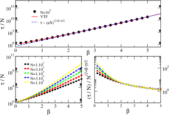
Figure 3: MFPT for scale-free uncorrelated random networks. Here $E_{0}=1$. Top: $\gamma=2.2$, $N=10^{5}$; both Eq.(13) and a VTF fit (with $T_{0}\approx 0.023$) are shown. Bottom: $\gamma=3$ and various network sizes. For $\beta<\beta_{c}=1$, $\tau\propto N$, while $\tau\propto N^{2+(\beta E_{0}-\gamma)/2}$ for $\beta>\beta_{c}$ .

and, using $k_{c}\sim m\log N$, we obtain $\langle{t_{MFPT}}\rangle\simeq N$ for $\beta E_{0}<1$ and $\langle{t_{MFPT}}\rangle\simeq N^{\beta E_{0}}$ for $\beta E_{0}>1$. Figure 3 shows the comparison of numerical data with the prediction of Eq. (13). The top panel also shows how, interestingly, a Vogel-Tammann-Fulcher form $\exp(A/(T-T_{0}))$ can also fit the data; however, the value of $T_{0}\sim 0.023$ has here no clear significance, while Eq. (13) provides a straightforward interpretation of the data.

In summary, we have put forward a simple mathematical model for the dynamics of glassy systems, seen as a random walk in a complex energy landscape. This work puts previous studies on the topology of the network of minima in a broader perspective and represents a first step towards a systematic integration of tools and concepts developed in complex network theory to the description of glassy dynamics in terms of the exploration of a phase space seen as a network of minima. It opens the way to studies on how network structures (such as community structures or bottlenecks, large clustering, non-trivial correlations) impact the dynamics. Other possible modifications of our model include taking into account fluctuations of the energies within a degree class (using for instance conditional energy distributions $P(E|k)$ instead of a relation $E=f(k)$), and other transition rates $r(k\to k^{\prime})$. A preliminary analysis shows that, for Glauber rates, the same phenomenology and the same necessary interplay between energy and degree described here are obtained. We also hope that this work will stimulate further detailed investigations on the relation between minima depth and connectivity.

Acknowledgments A. Baronchelli and R. P.-S. acknowledge financial support from the Spanish MEC (FEDER), under project No. FIS2007-66485-C02-01, as well as additional support through ICREA Academia, funded by the Generalitat de Catalunya. A. Baronchelli aknowledges support of Spanish MCI through the Juan de la Cierva programme.

References

- (1) P.G. Debenedetti and F.H. Stillinger, Nature 210, 259 (2001); Slow Relaxations and Nonequilibrium Dynamics in Condensed Matter, Les Houches Session LXXVII, 1-26 July, 2002 J.-L. Barrat et al. (Eds.), Springer (2003).
- (2) L. Angelani et al., Phys. Rev. Lett. 81, 4648 (1998); R. S. Berry and R. Breitengraser-Kunz, Phys. Rev. Lett. 74, 3951 (1995).
- (3) J.-P. Bouchaud, J. Physique I (France) 2 (1992) 1705.
- (4) C. Monthus and J.-P. Bouchaud, J. Phys. A 29, 3847 (1996).
- (5) M. Cieplak et al., Phys. Rev. Lett. 80, 3654 (1998).
- (6) L. Bongini et al., arXiv:0811.3148.
- (7) S. Carmi et al., J. Phys. A 42, 105101 (2009)
- (8) M. E. J. Newman, SIAM Review 45, 167 (2003); G. Caldarelli, Scale-Free Networks (Oxford University Press, Oxford, 2007).
- (9) A. Scala, L.A.N. Amaral, M. Barthélemy, Europhys. Lett. 55, 594 (2001).
- (10) J. P. K. Doye, Phys. Rev. Lett. 88, 238701 (2002).
- (11) C. P. Massen, J. P. K. Doye, Phys. Rev. E 71, 046101 (2005) Phys. Rev. E 75, 037101 (2007). J. Chem. Phys, 127, 114306 (2007).
- (12) H. Seyed-allaei, H. Seyed-allaei, M. Reza Ejtehadi, Phys. Rev. E 77, 031105 (2008).
- (13) J. P. K. Doye, C. P. Massen, J. Chem. Phys, 122, 084105 (2005).
- (14) D. Gfeller et al., Proc. Natl. Acad. Sci. (USA) 104, 1817 (2007); D. Gfeller et al., Phys. Rev. E 76, 026113 (2007); Z. Burda et al., Phys. Rev. E 73, 036110 (2006); Z. Burda, A. Krzywicki, O. C. Martin, Phys. Rev. E 76, 051107 (2007); M. Baiesi et al., arXiv:0812.0316 (2008).
- (15) S. N. Dorogovtsev, A. V. Goltsev, and J. F. F. Mendes, Rev. Mod. Phys. 80, 1275 (2008).
- (16) A. Barrat, M. Barthélemy, A. Vespignani, Dynamical processes on complex networks, Cambridge University Press, Cambridge (2008).
- (17) M. Catanzaro, M. Boguñá, and R. Pastor-Satorras, Phys. Rev. E 71, 027103 (2005).
- (18) S. Redner, A guide to first passage processes, Cambridge University Press, Cambridge (2001); J. D. Noh and H. Rieger Phys. Rev. Lett. 92, 118701 (2004); S. Condamin et al. Nature 450, 77- 80 (2007).