Role of nonlinear vector meson interactions in hyperon stars.

Abstract

The extended nonlinear model has been applied to construct neutron star matter equation of state. In the case of neutron star matter with non-zero strangeness the extension of the vector meson sector by the inclusion of nonlinear mixed terms results in the stiffening of the equation of state and accordingly in the higher value of the maximum neutron star mass.

1 Introduction

The analysis of the role of strangeness in nuclear structure in the aspect of multi-strange system is of great importance for both nuclear physics and for astrophysics. In the latter case understanding the properties of hyperon star is still a relevant item. At the core of a neutron star the matter density ranges from a few times the density of normal nuclear matter to about an order of a magnitude higher, at such densities exotic forms of matter such as hyperons are expected to emerge. The appearance of these additional degrees of freedom and their impact on a neutron star structure have been the subject of extensive studies [1], [2], [3], [4].
The description of a neutron star interior is modelled on the basis of the equation of state (EOS) of a dense nuclear system in a neutron rich environment. In general the description of nuclear matter is based on different models which can be grouped into phenomenological and microscopic. Additionally each one of them can be either relativistic or non-relativistic. In a microscopic approach the construction of the realistic model of nucleon-nucleon (NN) interaction can be inspired by the meson exchange theory of nuclear forces. The parameters within the model have to be adjusted to reproduce the experimental data for the deuteron properties and NN scattering phase shifts [5]. The solution of the nuclear many-body problem performed with the use of variational calculations for realistic NN interactions (for example for the Argonne v14 or Urbana v14 potentials) saturate at the density $\sim 2\times\rho_{0}$, where $\rho_{0}$ denotes the saturation density [6, 7]. In order to obtain the correct description of nuclear matter properties, namely the saturation density, binding energy and compression modulus at the empirical values, a phenomenological three-nucleon interaction has to be introduced. Two-body forces, together with implemented three-body forces, help providing the correct saturation point of symmetric nuclear matter [8]. The nuclear matter EOS calculated with the use of the Brueckner–Hartree–Fock [9], [10] approximation with the employed realistic two-nucleon interactions (the Bonn and Paris potentials) also does not correctly reproduce nuclear matter properties. Thus there are attempts to consider the nuclear interaction problem in a relativistic formalism. The relativistic version of the Brueckner–Hartree–Fock approximation – the Dirac–Brueckner–Hartree–Fock approach [11] is also based on realistic NN interactions. The nuclear EOS obtained from the DBHF approach using the Bonn A potential is soft at moderate densities but become stiffer at higher densities [12, 13]. At densities up to 2-3 times nuclear saturation density it is in agreement with constraints from heavy-ion collisions based on collective flow[14, 15] and kaon production [16].
The relativistic approach to nuclear matter at the hadronic energy scale developed by Walecka is very successful in describing a variety of the ground-state properties of finite nuclei at, or near the valley of stability and in predicting properties of exotic nuclei with large neutron to proton excess. The standard Walecka model [17] comprises nucleons interacting through the exchange of simulating medium range attraction $\sigma$ mesons and $\omega$ mesons responsible for the short range repulsion. Although this model properly described the saturation point and the data for finite nuclei it has been insufficient to properly describe the compression modulus of symmetric nuclear matter at saturation density $K_{v}$ and the proper density dependence in vector self-energy. The reproduced value of the incompressibility coefficient obtained in the original Walecka model gave large value of the order of $\sim 500$ MeV compared to the experimental results [18]. The nonlinear self-interactions of the scalar field (the cubic and quartic terms) have been added in order to get the acceptable value of the compression modulus $K_{v}$ [19, 20]. Its estimation made on the basis of recent experimental data point to the range $230\pm 10$ MeV [21, 22, 23, 24].
The quartic vector self-interaction softens the high density component of the EOS. This nonlinear term of the $\omega$ vector meson has been used by Sugahara and Toki to construct TM1 and TM2 models [25]. However, models which satisfactorily reproduce saturation properties of symmetric nuclear matter lead to considerable differences in the case when density and asymmetry dependence is included [26]. Isospin dependence of the strong interactions between nucleons influences both physical properties of nuclei and properties of infinite nuclear matter [27]. The latter case includes mainly the description of nuclear matter in high energy heavy-ion collisions and the properties of neutron star matter. Thus, the proper model of actual neutron star matter requires taking into consideration the effect of neutron-proton asymmetry. This in turn leads to the inclusion of the isovector meson $\rho$. The standard version of the $\rho$ meson field introduction is of a minimal type without any nonlinearities. This case has been further enlarged by the nonlinear mixed isoscalar-isovector couplings which modify the density dependence of the $\rho$ mean field and the energy symmetry. Such an extension of the neutron star model has been inspired by the paper [28] in which the authors show the existence of a relationship between the neutron-rich skin of a heavy nucleus and the properties of a neutron star crust.
The FSUGold model [29] which lead to considerably softer EOS. The meson sector of this model besides the linear terms of the scalar and vector fields includes nonlinear isoscalar meson self-interactions which soften the EOS of symmetric nuclear matter, and the mixed isoscalar-isovector coupling which alters the density dependence of the symmetry energy. Adding the mixed isoscalar-isovector meson interaction term the FSUGold model achieved acceptable results not only of the compression modulus for symmetric nuclear matter ($K_{v}=230$ MeV) but the value of the neutron skin in ²⁰⁸Pb of $R_{n}-R_{p}=0.21$ fm. The main astrophysical prediction of this model is connected with the value of the maximal neutron star mass which equals $M_{max}=1.72M_{\odot}$.
They are the nonlinear vector self-interactions that are discussed in this paper and the hadronic $SU(3)$ model which naturally includes nonlinear scalar and vector interaction terms is likely to be useful in the construction of models with nonzero strangeness and with more accurate description of asymmetric strangeness-rich neutron star matter [30]. The model considered has been extended to include a broad spectrum of nonlinear mixed vector meson couplings which stems from the very special form of the vector meson sector. The choice of these particular vector meson mixed interactions has been motivated by the chiral SU(3) model. The main effect of such an extension of the theory becomes evident when studying properties of neutron star matter, especially the form of the EOS. The equations of state for neutron star matter with hyperons considered in this paper have shown considerable stiffening for higher densities. Having obtained the equations of states the analysis of the maximum achievable neutron star mass for given class of models can be performed. Observational results limit the value of a neutron star mass and thereby put constraints on the EOS of high density nuclear matter. Recent observations of compact objects point to the existence of a high maximum neutron star mass [31]. The most spectacular result obtained with the Arecibo radio telescope for the neutron star-white dwarf binary system predicted the largest neutron star mass ever reported $M(PSRJ0751+1807)=2.1\pm 0.2M_{\odot}(1\sigma)$ [32]. However, this result has been corrected by Nice [13, 33]. The improved value of the orbital decay and the detection of the Shapiro delay lead to the new value $1.26M_{\odot}$ but with the estimated errors $1.12-1.30M_{\odot}(1\sigma)$ and $0.98-1.53M_{\odot}(2\sigma)$. Thus, this case can not be used as a constraint on the EOS. But there are another observations which indicate for high maximum mass of a neutron star. These are among others the value of the radius ($R>12$ km)of the isolated neutron star RX J1856.5-3754 [34] or neutron star mass in the low mass X-ray binary (LMXB) 4U 1636-536 estimated at the value of $2.0\pm 0.1M_{\odot}$ [35]. Another example of the LMXB is the neutron star in EXO 0748-676 which has been constrained by the detection of gravitational redshift of certain absorption lines. This combined with other observational data lead to individually estimated mass and radius of the star at the value of $M\geq 2.10\pm 0.28M_{\odot}$ and $R\geq 13.8\pm 1.8$ km [36, 37].

2 Constituents of the model

All calculations in this model have been done within the theoretical framework of quantum hadrodynamics (QHD) and the starting point is the nonlinear Walecka model which successfully describes the properties of nuclear matter and finite nuclei [17], [38]. Owing to substantial asymmetry of neutron star matter models which include additional isospin carrying terms can be used for its remarkably complete description. Such models with Lagrangian functions supplemented by isospin dependent nonlinear, mixed vector meson couplings have been introduced and analyzed in papers by Piekarewicz et al. [2], [28], [41]. In the model considered there are couplings which relate the $\omega$ and $\rho$ vector mesons with the $\phi$ meson and thus link the asymmetry of the system with the strangeness content. The inclusion of a broad spectrum of mixed nonlinear vector meson couplings provides the possibility of modifying the high density component of the EOS. However, the presence of additional terms in the Lagrangian function requires the adjustment of new coupling constants. This has been done by fitting to the properties of nuclear matter.
The presented model contains baryons and mesons as basic degrees of freedom. The baryon-meson interactions and meson-meson interactions are constructed on the basis of chiral SU(3) model [30].

2.1 Spin-0 meson fields

Additional hadronic states are produced in neutron star interiors in high density regime when the Fermi energy of nucleons exceeds the hyperon masses. The hadronic SU(3) [30] model which includes nonlinear scalar and vector interaction terms offers the possibility of constructing a strangeness rich neutron star model and of providing its detail description. The relevant degrees of freedom are hadrons - composite fields constructed from quarks. The problem considered is inspired by the chiral SU(3) model [30] in the nonlinear realization which influences transformational properties of quarks. The structure of hadrons is given in terms of their constituent quark fields $q$ which can be split into left $q_{L}$ and right-handed $q_{R}$ parts ($q=q_{L}+q_{R}$). They transform under $SU(3)_{L}\times SU(3)_{R}$ as

$$q_{L}\rightarrow q_{L}^{{}^{\prime}}=Lq_{L},\qquad q_{R}\rightarrow q_{R}^{{}^{\prime}}=Rq_{R}.$$ (1)

For the quarks of the nonlinear representation $\widetilde{q}$ the following relation can be written

$$q_{L}=u\widetilde{q}_{L}\qquad q_{R}=u^{{\dagger}}\widetilde{q}_{R}$$ (2)

where $\widetilde{q}_{L}$ and $\widetilde{q}_{R}(x)$ are left- and right-handed components of the quark field $\widetilde{q}$ and $u\equiv u(\pi(x))$ is given by

$$u(\pi(x))=\sum_{a=1}^{8}\exp{\left(\frac{i}{2\sigma_{0}}\pi^{a}(x)\lambda_{a}\right)}$$ (3)

with pseudoscalar mesons $\pi_{a}$ considered as parameters of the symmetry transformation. They are identify with the octet of physical pseudoscalar fields [30].
In general the meson content of the model consists of spin-0 and spin-1 mesons. Introducing the matrix field $\Phi$ enables the collective representation of the spin zero fields which in the matrix notation can be written as $\Phi=\Sigma+i\Pi$. The $\Sigma$ and $\Pi$ mesons can be transformed into nonlinearly transforming filds $X$ and $Y$

$$\Phi=\Sigma+i\Pi=u(X+iY)u,$$ (4)

where $X$ is associated with the scalar nonet and $Y$ with the pseudoscalar singlet which has to be added separately. The pseudoscalar mesons appear as the parameters of the symmetry transformation. The meson multiplets can be expanded in the basis of Gell-Mann matrices thus $\Phi=\frac{1}{\sqrt{2}}T_{a}\phi_{a}$ where $T_{a}=\lambda_{a}$ are generators of $U(3)$ and $\lambda_{a}$ (a=1…8) are the Gell-Mann matrices. It is convenient to introduce as a ninth matrix $\lambda_{0}=\sqrt{2/3}\,I$ ($I$ is a unit matrix). The set $\{i\lambda_{a}\}_{a=0,\ldots 8}$ constitutes a basis of the Lie algebra $u(3)$ of $U(3)$.
The scalar fields in the basis of $U(3)$ generators are not mass eigenstates. If the ideal mixing between the octet and singlet states has been assumed then the octet state $\sigma_{8}$ and the singlet state $\sigma_{0}$ are related to the ideal mixing states $\bar{\sigma}$ and $\bar{\zeta}$ of a scalar nonet through the orthogonal transformation

$$\left(\begin{array}[]{c}\bar{\sigma}\\ \bar{\zeta}\end{array}\right)=\left(\begin{array}[]{cc}cos\,\theta&sin\,\theta\\ -sin\,\theta&cos\,\theta\end{array}\right)\left(\begin{array}[]{c}\sigma_{8}\\ \sigma_{0}\end{array}\right).$$ (5)

Presenting the scalar multiplet as matrix the following form can be obtained

$$X=\left(\begin{array}[]{ccc}\frac{(a_{0}^{0}+\bar{\sigma})}{\sqrt{2}}&a_{0}^{+}&\kappa^{+}\\ a_{0}^{-}&\frac{(-a_{0}^{0}+\bar{\sigma})}{\sqrt{2}}&\kappa^{0}\\ \kappa^{-}&\bar{\kappa^{0}}&\bar{\zeta}\end{array}\right).$$ (6)

In the process of spontaneous chiral symmetry breaking $X$ acquires the vacuum expectation value (VEV) $\equiv<X>$. As only components proportional to $\lambda_{0}$ and the hypercharge $Y\sim\lambda_{8}$ are nonvanishing, $<X>$ takes the form $diag\{<\bar{\sigma}>,<\bar{\sigma}>,<\bar{\zeta}>\}$ and the following relations hold $f_{\pi}=\sqrt{<\bar{\sigma}>}$ and $f_{K}=(<\bar{\sigma}>+<\bar{\zeta}>)/\sqrt{2}$ where $f_{\pi}$ and $f_{K}$ are the pseudoscalar decay constants.
Making references to the Walecka model the following transformation should be done

$$\bar{\sigma} = \sigma+<\bar{\sigma}>$$ (7)

$$\bar{\zeta} = \sigma^{\ast}+<\bar{\zeta}>$$

where $\sigma$ and $\sigma^{\ast}$ denotes fields in the Walecka model.
In this paper the mean field approach serves as a method for solving the many body problem. In this approximation meson fields are separated into classical mean field values and quantum fluctuations, which are not included in the ground state. Thus, for the ground state of homogeneous infinite nuclear matter quantum fields operators are replaced by their classical expectation values $s_{0}$ and $s_{0}^{\ast}$

$$\sigma = \tilde{\sigma}+s_{0}$$ (8)

$$\sigma^{\ast} = \tilde{\sigma}^{\ast}+s_{0}^{\ast}.$$

2.2 Spin-1 meson fields

The spin-1 mesons are given by two octets of vector and axial vector fields. These fields similarly as in the case of spin zero mesons also can be written in a compact form

$$l_{\mu}(r_{\mu})=\frac{1}{2}(V_{\mu}\pm A_{\mu})=\frac{1}{2\sqrt{2}}\sum_{a=0}^{a=8}(v_{\mu}^{a}\pm a_{\mu}^{a})\lambda^{a},$$ (9)

where $l_{\mu}$ and $r_{\mu}$ corresponds to left and right-handed gauge fields, respectively and $V_{\mu}$ and $A_{\mu}$ denote the vector and axial vector nonets respectively.
The physical isoscalar $\omega$ and $\phi$ meson fields stem from the pure singlet $v_{\mu}^{0}$ and octet $v_{\mu}^{8}$ isoscalar states and can be obtained assuming ideal mixing, namely that $\phi_{\mu}$ is a pure $\bar{s}s$ state. This come down to the following relations

$$\phi_{\mu} = \frac{1}{\sqrt{3}}(\sqrt{2}v_{\mu}^{0}+v_{\mu}^{8})$$ (10)

$$\omega_{\mu} = \frac{1}{\sqrt{3}}(v_{\mu}^{0}-\sqrt{2}v_{\mu}^{8}).$$

Accordingly the vector meson multiplet can be expressed explicitly in terms of physical fields as

$$V_{\mu}=\left(\begin{array}[]{ccc}\frac{(\omega_{\mu}+\rho_{\mu}^{0})}{\sqrt{2}}&\rho_{\mu}^{+}&K^{\ast+}\\ \rho_{\mu}^{-}&\frac{(\omega_{\mu}+\rho_{\mu}^{0})}{\sqrt{2}}&K^{\ast 0}\\ K^{\ast-}&\overline{K}^{\ast 0}&\phi_{\mu}\end{array}\right).$$ (11)

2.3 Baryon fields

Nonlinearly transforming baryon fields can be written as

$$B_{L}=u^{{\dagger}}\Psi_{L}u\qquad B_{R}=u\Psi_{R}u^{{\dagger}}$$ (12)

where $\Psi_{L}$ and $\Psi_{R}$ are the left and right-handed parts of the baryon field in the linear representation. Baryon fields that enter the model are grouped into $3\times 3$ traceless matrix $\mathcal{B}$

$$\mathcal{B}=\left(\begin{array}[]{ccc}\frac{1}{\sqrt{6}}\Lambda+\frac{1}{\sqrt{2}}\Sigma^{0}&\Sigma^{+}&p\\ \Sigma^{-}&\frac{1}{\sqrt{6}}\Lambda-\frac{1}{\sqrt{2}}\Sigma^{0}&n\\ \Xi^{-}&\Xi^{0}&-\frac{2}{\sqrt{6}}\Lambda\end{array}\right).$$ (13)

3 The model

The dynamics of the system has been described in terms of the Lagrangian function which in its most general form can be given as a sum of two basic parts representing meson and baryon sectors which are directly related by the term defining the baryon-meson interaction

$$\mathcal{L}=\mathcal{L}_{kin}+\mathcal{L}_{M}+\mathcal{L}_{B}+\mathcal{L}_{BM}.$$ (14)

Additionally the kinetic term $\mathcal{L}_{kin}$ for both baryon and meson fields has been included.

3.1 The meson sector

The chiral SU(3) theory provides the basis for calculations made in this paper, however, the relativistic mean field approach to the description of the static, uniform nuclear matter leads to useful generalization about the model considered. In general, the meson sector includes contributions from spin zero and spin one mesons but in the mean field approximation vacuum expectation value of the pseudoscalar and axial meson fields vanishes and these fields do not enter to the Lagrangian function. In the result meson field Lagrangian $\mathcal{L}_{M}$ embodies only the parts for scalar and vector mesons

$$\mathcal{L}_{M}=\mathcal{L}_{S}+\mathcal{L}_{V}.$$ (15)

The scalar part of the Lagrangian function $\mathcal{L}_{M}$ includes the potential terms

$$\mathcal{L}_{S}=-k_{1}(I_{2})^{2}+k_{2}I_{4}+2k_{3}I_{3},$$ (16)

which are given in the form of chiral invariants defined as

$$I_{1}=Tr(X),\,\,I_{2}=Tr(X)^{2},\,\,I_{3}=detX.$$ (17)

The vector meson Lagrangian function presented in this model is the sum of a mass term and vector meson self-interaction terms up to fourth order in the fields

$$\mathcal{L}_{V}=\frac{1}{2}m_{v}^{2}Tr(V_{\mu}V^{\mu})+\mathcal{L}_{VV}.$$ (18)

The second part of (18) can be written in the form of invariants

$$\mathcal{L}_{VV}=\frac{1}{4}c\,(Tr(V^{\mu}V_{\mu}))^{2}+\frac{1}{2}d\,Tr[(V^{\mu}V_{\mu})^{2}]+\frac{1}{16}f[Tr(V^{\mu})]^{4},$$ (19)

where $V_{\mu}$ is the vector meson multiplet. In order to split the mass degeneracy for the meson nonet the following chiral invariant has to be added

$$\mathcal{L}_{MV}=\frac{1}{4}\mu Tr[V_{\mu\nu}V^{\mu\nu}X^{2}].$$ (20)

This together with the kinetic energy term, which will be introduced in section 3.3, leads to the following terms for different vector mesons

$$-\frac{1}{4}[1-\mu\frac{\bar{\sigma}^{2}}{2}](V_{\rho}^{\mu\nu})^{2}-\frac{1}{4}[1-\frac{1}{2}\mu(\frac{\bar{\sigma}^{2}}{2}+k^{2})](V_{K^{*}}^{\mu\nu})^{2}$$ (21)

$$-\frac{1}{4}[1-\mu\frac{\bar{\sigma}^{2}}{2}](V_{\omega}^{\mu\nu})^{2}-\frac{1}{4}[1-\mu k^{2}](V_{\phi}^{\mu\nu}).$$

As the coefficients are not equal unity the vector meson fields have to be renormalized by the factor $Z_{\omega}^{-1}(\bar{\sigma})=1-\mu\bar{\sigma}^{2}/2$. The mass terms of the vector mesons differ from the mean mass $m_{V}$ by the renormalization factor and the following result can be obtained

$$m_{\omega}^{2}=m_{\rho}^{2}=Z_{\omega}(\sigma_{0})m_{V}^{2};\quad m_{K^{\ast}}^{2}=Z_{K^{\ast}}(\zeta_{0})m_{V}^{2};\quad m_{\phi}^{2}=Z_{\phi}(\zeta_{0})m_{V}^{2}$$ (22)

where the constants $m_{V}$ $\mu$ and $k$ are fixed to give the correct $\omega$ and $\phi$ masses and $\sigma_{0}=<\bar{\sigma}>|_{n_{B}=0}$ and $\zeta_{0}=<\bar{\zeta}>|_{n_{B}=0}$, $n_{B}$ denotes the baryon number density.
The baryonic part of the Lagrangian can be written as

$$\mathcal{L}_{B}=Tr(\bar{\mathcal{B}}i\gamma^{\mu}D_{\mu}\mathcal{B}),$$ (23)

where $\mathcal{B}$ is a $3\times 3$ traceless hermitian matrix given by relation (13) and $D_{\mu}$ denotes the covariant derivative of $\mathcal{B}$ which is defined as

$$D_{\mu}\mathcal{B}=\partial_{\mu}\mathcal{B}+i[\Gamma_{\mu},\mathcal{B}]$$ (24)

with $\Gamma_{\mu}$ defined as

$$\Gamma_{\mu}=-\frac{i}{2}[u^{{\dagger}}(\partial_{\mu}+ig_{v}l_{\mu})u+u(\partial_{\mu}+ig_{v}r_{\mu})u^{{\dagger}}].$$ (25)

3.2 Baryon-meson interaction

Using the notation introduced by [30] the very general SU(3) structure for the baryon-meson interaction can be written as

$$\mathcal{L}_{BM} = -\sqrt{2}g_{8}^{W}(\alpha_{W}[\bar{\mathcal{B}}\mathcal{O}\bar{B}W]_{F}+(1-\alpha_{W})[\bar{\mathcal{B}}\mathcal{O}\bar{\mathcal{B}}W]_{D})$$

$$- g_{1}^{W}\frac{1}{\sqrt{3}}Tr(\bar{\mathcal{B}}\mathcal{O}\mathcal{B})TrW,$$

where $W$ denotes general meson field and

$$[\bar{\mathcal{B}}\mathcal{O}\mathcal{B}W]_{F}:=Tr(\bar{\mathcal{B}}\mathcal{O}W\mathcal{B}-\bar{\mathcal{B}}\mathcal{O}\mathcal{B}W)$$ (27)

$$[\bar{\mathcal{B}}\mathcal{O}\mathcal{B}W]_{D}:=Tr(\bar{\mathcal{B}}\mathcal{O}W\mathcal{B}+\bar{\mathcal{B}}\mathcal{O}\mathcal{B}W)-\frac{2}{3}Tr(\bar{\mathcal{B}}\mathcal{O}\mathcal{B})TrW.$$ (28)

Different forms of the presented above interaction terms result from differences in the Lorentz structure.
For the nonlinear realization of chiral symmetry the antisymmetric (F-type) and symmetric (D-type) interaction terms of baryons not only with spin-1 but with spin-0 mesons as well are allowed.
In the case of baryon-scalar meson interaction $W=X,\mathcal{O}=\mathcal{I}$, for vector meson $W=V_{\mu},\mathcal{O}=\gamma_{\mu}$, for axial vector mesons $W=\mathcal{A_{\mu}},\mathcal{O}=\gamma_{\mu}\gamma_{5}$ and for pseudo-scalar mesons $W=u_{\mu},\mathcal{O}=\gamma_{\mu}\gamma_{5}$.
Baryon-spin zero meson interaction is indispensable for the construction of baryon mass terms. Masses of the whole baryon multiplet are generated spontaneously by the vacuum expectation values (VEV) of the non-strange and strange scalar fields. When the nucleon mass depends on the strange condensate $<\bar{\zeta}>$ the parameters $g_{1}^{S},g_{8}^{S}$ and $\alpha_{S}$ enable baryon masses to be fitted to their experimental values

$$m_{N}(\bar{\sigma},\bar{\zeta}) = m_{0}-\frac{1}{3}g_{8}^{S}(4\alpha_{S}-1)(\sqrt{2}\bar{\zeta}-\bar{\sigma})$$ (29)

$$m_{\Lambda}(\bar{\sigma},\bar{\zeta}) = m_{0}-\frac{2}{3}g_{8}^{S}(\alpha_{S}-1)(\sqrt{2}\bar{\zeta}-\bar{\sigma})$$

$$m_{\Sigma}(\bar{\sigma},\bar{\zeta}) = m_{0}+\frac{2}{3}g_{8}^{S}(4\alpha_{S}-1)(\sqrt{2}\bar{\zeta}-\bar{\sigma})$$

$$m_{\Xi}(\bar{\sigma},\bar{\zeta}) = m_{0}+\frac{1}{3}g_{8}^{S}(2\alpha_{S}+1)(\sqrt{2}\bar{\zeta}-\bar{\sigma}),$$

where $m_{0}$ is determined by two meson field condensates and is given by

$$m_{0}=g_{1}^{S}\frac{\sqrt{2}<\bar{\sigma}>+<\bar{\zeta}>}{\sqrt{3}}.$$ (30)

However, the assumption that $\alpha_{S}=1$ and $g_{1}^{S}=\sqrt{6}g_{8}^{S}$ leads to the model in which nucleon mass depends only on the nonstrange condensate $<\bar{\sigma}>$. In this case the coupling constance between the baryons and the two scalar condensates are related to the additive quark model. Then nucleon mass depends only on the non-strange condensate $<\bar{\sigma}>$, and only one coupling constant is needed to reproduce the correct value of the nucleon mass. To obtain the correct masses of the remaining baryons an explicit symmetry breaking term has to be added.
The explicit symmetry breaking term presented in the paper by [30] has been used

$$\mathcal{L}_{\Delta m}=-m_{1}Tr(\bar{\mathcal{B}}\mathcal{B}-\bar{\mathcal{B}}\mathcal{B}S)-m_{2}Tr(\bar{\mathcal{B}}S\mathcal{B})$$ (31)

where $S_{b}^{a}=1/3(\sqrt{3}(\lambda_{8})_{a}^{b}-\delta_{b}^{a})$ and the parameters $g_{8}^{S},m_{1}$ and $m_{2}$ are used to determine baryon masses:

$$m_{N} = -g_{N\sigma}<\bar{\sigma}>$$ (32)

$$m_{\Xi} = -\frac{1}{3}g_{N\sigma}<\bar{\sigma}>-\frac{2}{3g_{N\sigma}}\sqrt{2}\bar{<\zeta>}+m_{1}+m_{2}$$

$$m_{\Lambda} = -\frac{2}{3}g_{N\sigma}<\bar{\sigma}>-\frac{1}{3g_{N\sigma}}\sqrt{2}\bar{<\zeta>}+\frac{m_{1}+2m_{2}}{3}$$

$$m_{\Sigma} = -\frac{2}{3}g_{N\sigma}<\bar{\sigma}>-\frac{1}{3g_{N\sigma}}\sqrt{2}\bar{<\zeta>}+m_{1}.$$

Considering the case when nucleon mass depends only on non-strange condensate and once again making references to the Walecka model the relation for the baryon masses can be expressed as

$$m_{B}(\bar{\sigma},\bar{\zeta})=m_{B}(\sigma,\sigma^{\ast})=m_{B}-g_{B\sigma}\sigma-g_{B\sigma^{\ast}}\sigma^{\ast},$$ (33)

where the terms $g_{B\sigma}\sigma$ and $g_{B\sigma^{\ast}}\sigma^{\ast}$ represent the modification of baryon masses due to the medium.
The interaction of baryons with spin-1 mesons can be construct analogously with the baryon spin-0 meson interaction. For the case of pure F-type coupling ($\alpha_{V}=1$) the assumption $g_{1}^{V}=\sqrt{6}g_{8}^{V}$ (the strange vector field $\phi_{\mu}\sim\overline{s}\gamma_{\mu}s$ does not couple to nucleon) can be made. As it has been stated in the mean field approach the VEV of axial mesons are zero thus taking into account only vector mesons the Lagrangian describing baryon-vector meson interaction is given by

$$\mathcal{L}_{BV}=-\sqrt{2}g_{8}^{V}\left(Tr\bar{\mathcal{B}}\gamma^{\mu}[V_{\mu}^{8},\mathcal{B}]+Tr\bar{\mathcal{B}}\gamma^{\mu}\mathcal{B}\cdot TrV_{\mu}^{1}\right)$$ (34)

After insertion of the matrix (11) to equation (34) and using all the facts concerning the construction of the baryon mass the following form of the Lagrangian function can be written

$$\mathcal{L}_{MB}=Tr(\bar{\mathcal{B}}(i\gamma^{\mu}D_{\mu}-m_{B}(\bar{\sigma},\bar{\zeta}))\mathcal{B})$$ (35)

where $m_{B}$ denotes the mass of the baryon octet in the chiral limit and the covariant derivative of $\mathcal{B}$ is given by

$$D_{\mu}\mathcal{B}=\partial_{\mu}\mathcal{B}+i[\Gamma_{\mu},\mathcal{B}],$$ (36)

with the connection $\Gamma_{\mu}$.
In the vector meson sector the couplings to the strange baryons determined from the symmetry relations read

$$g_{N\omega} = (4\alpha_{V}-1)g_{8}^{V}$$ (37)

$$g_{\Lambda\omega} = \frac{2}{3}(5\alpha_{V}-2)g_{8}^{V}\qquad g_{\Lambda\phi}=-\frac{\sqrt{2}}{3}(2\alpha_{V}+1)g_{8}^{V}$$

$$g_{\Sigma\omega} = 2\alpha_{V}g_{8}^{V}\qquad g_{\Sigma\phi}=-2\sqrt{2}(2\alpha_{V}-1)g_{8}^{V}$$

$$g_{\Xi\omega} = (2\alpha_{V}-1)g_{8}^{V}\qquad g_{\Xi\phi}=-2\sqrt{2}\alpha_{V}g_{8}^{V}$$

Taking $\alpha_{V}=1$ the coupling constants related to the additive quark model can be obtained

$$g_{\Lambda\omega}=g_{\Sigma\omega}=g_{\Xi\omega}=\frac{2}{3}g_{N\omega}=2g_{8}^{V}\qquad g_{\lambda\phi}=g_{\Sigma\phi}=\frac{g_{\Xi\phi}}{2}=\frac{\sqrt{2}}{3}g_{N\omega}.$$ (38)

Similar symmetry relations can be obtained for the coupling constants in the scalar sector. These however are not used in the presented model. The couplings of baryons with the scalar mesons are determined from the experimentally estimated value of the $\Lambda$ central potential.

3.3 Kinetic terms

The explicit form of the baryon and meson kinetic terms are given by

$$\mathcal{L}_{kin}=iTr(\bar{\mathcal{B}}\gamma_{\mu}D^{\mu}\mathcal{B})+\frac{1}{2}Tr(D_{\mu}XD^{\mu}X)-\frac{1}{4}Tr(V_{\mu\nu}V^{\mu\nu})$$ (39)

where $D_{\mu}$ denotes the covariant derivative

$$D_{\mu}=\partial_{\mu}+i[\Gamma_{\mu},]$$ (40)

and $\Gamma_{\mu}$ is given by relation (25). The chirally invariant kinetic term for spin-1 mesons, in the case of vector mesons, is $V_{\mu\nu}=D_{\mu}V_{\nu}-D_{\nu}V_{\mu}$. The covariant derivative $D_{\mu}$ is given by relation (40).

4 The effective model

Vector mesons and thereby vector densities are the decisive factors that contribute to the EOS of dense matter in neutron star interiors. Thus, attention is focused on the construction of a model which includes wide spectrum of nonlinear couplings between vector meson fields. This allows one to perform a systematic analysis of their influence on the high density EOS.
As has been stated in previous section theoretical description of strange hadronic matter requires the extension of the nonlinear Walecka model by the inclusion of baryons of the lowest SU(3) flavor octet. In order to describe the strongly attractive $\Lambda\Lambda$ interaction two additional meson fields, the scalar meson $f_{0}(975)$ denoted as $\sigma^{\ast}$ and the vector meson $\phi(1020)$ have been introduced [39].
Thus, in the scalar meson sector besides non-strange $\sigma$ meson the hidden-strange $\sigma^{\ast}$ scalar meson is included whereas, in the case of vector mesons $\omega$, $\rho$ and $\phi$ mesons are comprised.
Summing-up the Lagrangian function for the system consists of a baryonic part which includes the full octet of baryons together with terms describing interaction of baryons with scalar and vector mesons and a mesonic part. The mesonic part contains also additional interactions between mesons which mathematically express themselves as supplementary, nonlinear terms in the Lagrangian function. Considering individual constituents of the model which have been described in the previous paragraph the very general form of Lagrangian function can be written

$${\mathcal{L}_{BM}}=\sum_{B}\bar{\psi}_{B}i\gamma^{\mu}D_{\mu}\psi_{B}-\sum_{B}m_{B}(\sigma,\sigma^{\ast})\overline{\psi}_{B}\psi_{B}+\mathcal{L}_{M},$$ (41)

where baryon fields $\Psi_{B}^{T}=(\psi_{N},\psi_{\Lambda},\psi_{\Sigma},\psi_{\Xi})$ are composed of the following isomultiplets [1]:

$$\begin{array}[]{cc}{\displaystyle\Psi_{N}={\psi_{p}\choose\psi_{n}},}&{\displaystyle\Psi_{\Lambda}=\psi_{\Lambda},}\\ \\ {\displaystyle\Psi_{\Sigma}=\left(\begin{array}[]{c}\psi_{\Sigma^{+}}\\ \psi_{\Sigma^{0}}\\ \psi_{\Sigma^{-}}\end{array}\right),}&{\displaystyle\Psi_{\Xi}={\psi_{\Xi^{0}}\choose\psi_{\Xi^{-}}},}\end{array}$$

$D_{\mu}$ is the covariant derivative of baryons which in terms of $\omega_{\mu},\rho_{\mu}^{a}$ and $\phi_{\mu}$ fields is given by

$$D_{\mu}=\partial_{\mu}+ig_{\omega B}\omega_{\mu}+ig_{\phi B}\phi_{\mu}+ig_{\rho B}I_{3B}\tau^{a}\rho_{\mu}^{a}.$$ (42)

The meson part of the Lagrangian function

$$\mathcal{L}_{M}=\frac{1}{2}\partial_{\mu}\sigma\partial^{\mu}\sigma+\frac{1}{2}\partial_{\mu}\sigma^{\ast}\partial^{\mu}\sigma^{\ast}-U_{eff}(\sigma,\sigma^{\ast},\omega_{\mu},\rho_{\mu}^{a},\phi_{\mu})$$

$$-\frac{1}{4}\Omega_{\mu\nu}\Omega^{\mu\nu}-\frac{1}{4}R_{\mu\nu}^{a}R^{a\mu\nu}-\frac{1}{4}\Phi_{\mu\nu}\Phi^{\mu\nu}$$ (43)

includes the field tensors $\Omega_{\mu\nu},\Phi_{\mu\nu}$ and $R_{\mu\nu}^{a}$ defined as

$$\Omega_{\mu\nu}=\partial_{\mu}\omega_{\nu}-\partial_{\nu}\omega_{\mu}\hskip 14.22636pt\Phi_{\mu\nu}=\partial_{\mu}\phi_{\nu}-\partial_{\nu}\phi_{\mu}$$ (44)

$$R_{\mu\nu}^{a}=\partial_{\mu}\rho_{\nu}^{a}-\partial_{\nu}\rho_{\mu}^{a}.$$ (45)

All meson interaction terms are collected in the potential function $U_{eff}(\sigma,\sigma^{\ast},\omega_{\mu},\rho_{\mu}^{a},\phi_{\mu})$ which can be written as a sum of linear and nonlinear parts

$$\mathcal{U}_{eff}(\sigma,\sigma^{\ast},\omega_{\mu},\rho_{\mu}^{a},\phi_{\mu})=\mathcal{U}_{lin}(\sigma,\sigma^{\ast},\omega_{\mu},\rho_{\mu}^{a},\phi_{\mu})+\mathcal{U}_{nl}(\sigma,\sigma^{\ast},\omega_{\mu},\rho_{\mu}^{a},\phi_{\mu}).$$ (46)

The linear scalar and vector meson part of the potential takes the form

$$\mathcal{U}_{lin}(\sigma,\sigma^{\ast},\omega_{\mu},\rho_{\mu}^{a},\phi_{\mu}) = \frac{1}{2}m_{\sigma}^{2}\sigma^{2}+\frac{1}{2}m_{\sigma^{\ast}}^{2}\sigma^{\ast 2}-\frac{1}{2}m_{\omega}^{2}(\omega_{\mu}\omega^{\mu})$$

$$- \frac{1}{2}m_{\rho}^{2}(\rho_{\mu}^{a}\rho^{\mu a})-\frac{1}{2}m_{\phi}^{2}(\phi_{\mu}\phi^{\mu}),$$

whereas its nonlinear part is given by

$$\mathcal{U}_{nl}(\sigma,\sigma^{\ast},\omega_{\mu},\rho_{\mu}^{a},\phi_{\mu})=\frac{1}{3}g_{3}\sigma^{2}+\frac{1}{4}g_{4}\sigma^{4}+\frac{1}{4}(c+2d+\frac{1}{4}f)(\phi_{\mu}\phi^{\mu})^{2}+$$ (48)

$$+\frac{1}{4}(c+d)(\rho_{\mu}^{a}\rho^{\mu a})^{2}+\frac{1}{2}c(\rho_{\mu}^{a}\rho^{\mu a})(\phi_{\nu}\phi^{\nu})+\frac{1}{2\sqrt{2}}f(\omega_{\mu}\phi^{\mu})(\phi_{\nu}\phi^{\nu})+$$

$$+\frac{1}{2}(c(\rho_{\mu}^{a}\rho^{\mu a})+3d(\rho_{\mu}^{a}\rho^{\mu a})+c(\phi_{\mu}\phi^{\mu})+\frac{3}{2}f(\phi_{\mu}\phi^{\mu})(\omega_{\nu}\omega^{\nu}))+$$

$$+\frac{1}{\sqrt{2}}f(\phi_{\mu}\omega^{\mu})(\omega_{\nu}\omega^{\nu})+\frac{1}{4}(c+d+f)(\omega_{\mu}\omega^{\mu})^{2}.$$

The potential function $\mathcal{U}_{eff}(\sigma,\sigma^{\ast},\omega_{\mu},\rho_{\mu}^{a},\phi_{\mu})$ includes subsets of non-strange and strangeness rich matter and this can be written with the use of the following notation

$$\mathcal{U}_{eff}(\sigma,\sigma^{\ast},\omega_{\mu},\rho_{\mu}^{a},\phi_{\mu})=\mathcal{U}_{i,S=0}+\mathcal{U}_{i,S\neq 0},$$ (49)

where $i$ denotes linear and non-linear parts of the potential (46). If strangeness bearing components are not taking into account in the description of matter and only nucleons are considered, the Lagrangian density function constructed on the basis of the Walecka model can be retained which in the case of symmetric matter comprises contributions coming from nucleons, $\sigma$ and $\omega_{\mu}$ mesons. As neutron star matter is highly asymmetric one the inclusion of isovector-vector meson $\rho_{\mu}^{a}$ become indispensable. Finally making reference to the extended Walecka model with nonlinear scalar and vector meson self-interaction terms the Lagrangian function can be presented as follows

$$\mathcal{L} = \bar{\psi}_{N}(i\gamma^{\mu}D_{\mu}-(m_{N}(\sigma)-g_{\sigma N}\sigma))\psi_{N}+\frac{1}{2}\partial_{\mu}\sigma\partial^{\mu}\sigma-$$ (50)

$$- \frac{1}{4}\Omega_{\mu\nu}\Omega^{\mu\nu}-\frac{1}{4}R_{\mu\nu}^{a}R^{a\mu\nu}+\frac{1}{2}m_{\omega}^{2}\omega_{\mu}\omega^{\mu}$$

$$+ \frac{1}{2}m_{\rho}\rho_{\mu}^{a}\rho^{a\mu}-U_{eff,S=0}(\sigma,\omega_{\mu},\rho_{\mu}^{a})$$

where

$$\psi_{N}=\left(\begin{array}[]{c}\psi_{p}\\ \psi_{n}\end{array}\right)$$

is the nucleon field, $D_{\mu}$ denotes the covariant derivative which now reduces to

$$D_{\mu}=\partial_{\mu}+ig_{\omega N}\omega_{\mu}+ig_{\rho N}I_{3N}\tau^{a}\rho_{\mu}^{a}.$$ (51)

The nucleon mass is denoted by $m_{N}(\sigma)$ $(N=n,p)$ whereas $m_{i}$ $(i=\sigma,\omega,\rho)$ are masses assigned to the meson fields, $R_{\mu\nu}^{a}$ and $\Omega_{\mu\nu}$ again denotes the field tensors and are given by (44) and (45).
Collecting all the meson self-interactions and the mixed $\omega-\rho$ and $\sigma-\rho$ terms in the model considered a nonlinear part of the potential $U_{eff,S=0}(\sigma,\omega_{\mu},\rho_{\mu}^{a})$ can be specified

$$U_{nl,S=0}(\sigma,\omega_{\mu},\rho_{\mu}^{a})=-\frac{\kappa}{3!}\sigma^{3}-\frac{\lambda}{4!}\sigma^{4}+c_{3}(\omega_{\mu}\omega^{\mu})^{2}$$ (52)

$$+\frac{\zeta}{4!}g_{\rho N}^{4}(\rho_{\mu}^{a}\rho^{\mu a})^{2}+\Lambda_{V}(g_{\omega N}g_{\rho N})^{2}(\omega_{\mu}\omega^{\mu})(\rho_{\mu}^{a}\rho^{\mu a})+\Lambda_{4}(g_{\sigma N}g_{\rho N})^{2}\sigma^{2}(\rho_{\mu}^{a}\rho^{\mu a}).$$

More detailed analysis of the vector meson influence on the high density EOS needs to consider different types of nonlinear vector meson couplings.
The very general form of the vector meson Lagrangian (19) includes the potential which is defined by coupling constants that appeared in the vector meson Lagrangian (19). Since the coupling constants of the mixed vector meson interactions are known very poorly, if ever, there are still important uncertainties in the analysis of their influence on the form of the EOS. In order to study the importance of individual parts of the potential it is necessary to find connections between the coupling constants $c$, $d$ and $f$ and the couplings in the vector part of the nonlinear potential $U_{nl}(\sigma,\omega_{\mu},\rho_{\mu}^{a})$.
The results reveal the following relations

$$c=\frac{1}{2}(3c_{3}-3c_{3}\beta-2g_{\rho}^{2}g_{\omega}^{2}\Lambda_{V})$$ (53)

$$d=\frac{1}{2}(-c_{3}+c_{3}\beta+2g_{\rho}^{2}g_{\omega}^{2}\Lambda_{V})$$ (54)

$$f=c_{3}\beta.$$ (55)

In the paper by Serot et. al [40] the acceptable values of the parameters entering the very general nonlinear model have been introduced. In accordance with the estimations made in the paper [40] a new parameter $\beta$ which takes the value in the range <0;1> can be introduced. This parameter makes possible to carry out more systematic analysis and to include wider class of models that have been constructed on the basis of the invariants presented in (19). The considered cases lead to models and results which already have been reported. Incorporating the relations (53-55) the vector potential can be constructed

$$\mathcal{U}_{V} = \frac{1}{4}c_{3}\left((\rho_{\mu}^{a}\rho^{\mu a})^{2}(1-\beta)+(\omega_{\mu}\omega^{\mu})^{2}\right)+$$

$$+ (\omega_{\mu}\omega^{\mu})\left(\frac{3}{4}c_{3}(\phi_{\mu}\phi^{\mu})+\frac{1}{2}(g_{\rho}g_{\omega})^{2}\Lambda_{V}(2(\rho_{\mu}^{a}\rho^{\mu a})-(\phi_{\mu}\phi^{\mu})\right)+$$

$$+ (\rho_{\mu}^{a}\rho^{\mu a})\left(\frac{3}{4}c_{3}(\phi_{\mu}\phi^{\mu})-\frac{3}{4}\beta\phi_{\mu}\phi^{\mu}-\frac{1}{2}(g_{\rho}g_{\omega})^{2}\Lambda_{V}\phi_{\mu}\phi^{\mu}\right)+$$

$$+ \frac{1}{8}(\phi_{\mu}\phi^{\mu})^{2}\left(c_{3}(1-\frac{1}{2}\beta)+2(g_{\omega}g_{\rho})^{2}\Lambda_{V}\right)$$

$$+ \frac{3}{4}c_{3}(\rho_{\mu}^{a}\rho^{\mu a})(\phi_{\mu}\phi^{\mu})(1-\beta)+\frac{1}{2\sqrt{2}}\beta c_{3}(\phi_{\nu}\phi^{\nu})(\phi_{\mu}\omega^{\mu})+$$

$$+ \frac{3}{4}c_{3}(\phi_{\mu}\phi^{\mu})(\omega_{\mu}\omega^{\mu})+\frac{1}{\sqrt{2}}\beta c_{3}(\phi_{\mu}\omega^{\mu})(\omega_{\nu}\omega^{\nu}).$$

Detailed analysis of the presented above potential can be made considering different cases.

1.

Nonstrange matter $(S=0)$. This case includes variety of models and leads directly to the well-known results presented in the literature.
The potential (4) reduces to the most general form for non-strange matter

$$\mathcal{U}_{V}=\frac{1}{4}c_{3}(\rho_{\mu}^{a}\rho^{\mu a})^{2}\left(1-\beta\right)+\frac{1}{4}c_{3}(\omega_{\mu}\omega^{\mu})^{2}+(g_{\rho}g_{\omega})^{2}\Lambda_{V}(\rho_{\mu}^{a}\rho^{\mu a})(\omega_{\mu}\omega^{\mu}).$$ (57)

The analysis starts with the case $\beta=0$ and $\Lambda_{V}=0$.

$$\mathcal{U}_{V}=\frac{1}{4}c_{3}(\rho_{\mu}^{a}\rho^{\mu a})^{2}+\frac{1}{4}c_{3}(\omega_{\mu}\omega^{\mu})^{2}$$ (58)

includes contributions from both isoscalar and isovector components. The last one is of special interest for the the asymmetric neutron star matter.
The case with $\Lambda_{V}\neq 0$

$$\mathcal{U}_{V}=\frac{1}{4}c_{3}(\rho_{\mu}^{a}\rho^{\mu a})^{2}+\frac{1}{4}c_{3}(\omega_{\mu}\omega^{\mu})^{2}+(g_{\rho}g_{\omega})^{2}\Lambda_{V}(\rho_{\mu}^{a}\rho^{\mu a})(\omega_{\nu}\omega^{\nu}).$$ (59)

This form of the potential function incorporates additional vector meson mixed term.
The case with $\beta=1$ and $\Lambda_{V}\neq 0$

$$\mathcal{U}_{V}=\frac{1}{4}c_{3}(\omega_{\mu}\omega^{\mu})^{2}+(g_{\rho}g_{\omega})^{2}\Lambda_{V}(\rho_{\mu}^{a}\rho^{\mu a})(\omega_{\nu}\omega^{\nu})$$ (60)

This is the model studied by Piekarewicz et al. [28], [41]
The case with $\beta=1$ and $\Lambda_{V}=0$

$$\mathcal{U}_{V}=\frac{1}{4}c_{3}(\omega_{\mu}\omega^{\mu})^{2}$$ (61)

The nonlinear Walecka model is retained in this situation.

2.

Matter with nonzero strangeness $(S\neq 0)$.
The case with $\beta=0$

$$\mathcal{U}_{V} = \frac{1}{4}c_{3}(\rho_{\mu}^{a}\rho^{\mu a})^{2}+\frac{3}{4}c_{3}(\rho_{\mu}^{a}\rho^{\mu a})(\phi_{\nu}\phi^{\nu})+\frac{1}{8}c_{3}(\phi_{\mu}\phi^{\nu})^{2}$$

$$+\frac{3}{4}c_{3}(\phi_{\mu}\phi^{\mu})(\omega_{\nu}\omega^{\nu})+\frac{1}{4}(g_{\rho}g_{\omega})^{2}\Lambda_{V}(\phi_{\mu}\phi^{\mu})^{2}$$

$$+\frac{1}{4}c_{3}(\omega_{\mu}\omega^{\mu})^{2}-\frac{1}{2}(g_{\rho}g_{\omega})^{2}\Lambda_{V}(\rho_{\mu}^{a}\rho^{\mu a})(\phi_{\nu}\phi^{\nu})$$

$$+(g_{\rho}g_{\omega})^{2}\Lambda_{V}(\rho_{\mu}^{a}\rho^{\mu a})(\omega_{\nu}\omega^{\nu})-\frac{1}{2}(g_{\rho}g_{\omega})^{2}\Lambda_{V}(\phi_{\mu}\phi^{\mu})(\omega_{\nu}\omega^{\nu})$$

The case with $\beta=0$ and $\Lambda_{V}=0$

$$\mathcal{U}_{V} = \frac{1}{4}c_{3}(\rho_{\mu}^{a}\rho^{\mu a})^{2}+\frac{3}{4}c_{3}(\rho_{\mu}^{a}\rho^{\mu a})(\phi_{\nu}\phi^{\nu})$$ (63)

$$+ \frac{1}{8}c_{3}(\phi_{\mu}\varphi^{\mu})^{2}+\frac{3}{4}c_{3}(\phi_{\mu}\phi^{\mu})(\omega_{\nu}\omega^{\nu})$$

The case with $\beta=1$ and $\Lambda_{V}\neq 0$

$$\mathcal{U}_{V} = \frac{1}{16}c_{3}(\phi_{\mu}\phi^{\mu})^{2}++\frac{1}{2\sqrt{2}}c_{3}(\phi_{\mu}\phi^{\mu})(\phi_{\nu}\omega^{\nu})+\frac{3}{4}c_{3}(\phi_{\mu}\phi^{\mu})(\omega_{\nu}\omega^{\nu})$$ (64)

$$+ \frac{1}{\sqrt{2}}c_{3}(\phi_{\mu}\omega^{\mu})(\omega_{\nu}\omega^{\nu})+\frac{1}{4}c_{3}(\omega_{\mu}\omega^{\mu})^{2}-\frac{1}{2}(g_{\rho}g_{\omega})^{2}\Lambda_{V}(\rho_{\mu}^{a}\rho^{\mu a})(\phi_{\nu}\phi^{\nu})$$

$$+ \frac{1}{4}(g_{\rho}g_{\omega})^{2}\Lambda_{V}(\phi_{\mu}\phi^{\mu})^{2}$$

$$+ (g_{\rho}g_{\omega})^{2}\Lambda_{V}\rho_{\mu}^{2}(\omega_{\mu}\omega^{\mu})-\frac{1}{2}(g_{\rho}g_{\omega})^{2}\Lambda_{V}(\phi_{\mu}\phi^{\mu})(\omega_{\nu}\omega^{\nu})$$

The case with $\beta=1$ and $\Lambda_{V}=0$

$$\mathcal{U}_{V} = \frac{1}{16}c_{3}(\phi_{\mu}\phi^{\mu})^{2}+\frac{1}{2\sqrt{2}}c_{3}(\phi_{\mu}\phi^{\mu})(\phi^{\nu}\omega_{\nu})+$$

$$+ \frac{3}{4}c_{3}(\phi_{\mu}\phi^{\mu})(\omega_{\nu}\omega^{\nu})+\frac{1}{\sqrt{2}}c_{3}(\phi_{\mu}\omega^{\mu})(\omega_{\nu}\omega^{\nu})+\frac{1}{4}c_{3}(\omega_{\mu}\omega^{\mu})^{2}.$$

Summing up the vector meson potential in general can include a wide variety of nonlinear terms. The presence of nonzero strangeness led to very distinct division of the constructed models. This has been done with the use of the parameter $\beta$. For nucleonic matter ($S=0$) both cases $\beta=0$ and $\beta=1$ have been analyzed. The latter one is of special importance as it enables the comparison of the results with those obtained by Piekarewicz et al. [41]. However, in the case of nonzero strangeness important reduction has been done. Models constructed for the case $\beta=1$ lead to very soft equation of state and consequently to very low value of the maximum neutron star masses. This is not interested according to results of recent observations which point towards larger masses. Such masses are especially concerned about the stiffening of the EOS at sufficiently high densities. This stiffening of the equation of state has become a big issue particularly for strangeness rich matter. Thus, further analysis of the influence of the nonlinear vector meson interactions for strangeness rich matter will concentrate on the case with $\beta=0$.

4.1 Mean Field Approximation

The system considered, has been assumed to be isotropic, infinite matter in its ground state. To investigate properties of infinite nuclear matter, the mean field approximation has been adopted. The symmetries of infinite nuclear matter simplify the model to a great extent. The translational and rotational invariance claimed that the mean fields of all the vector fields vanish. Only the time-like components of the neutral vector mesons have a non-vanishing expectation value. Owing to parity conservation, the vacuum expectation value of pseudoscalar fields vanish ($<\pi_{a}>=0$). Meson fields have been separated into classical mean field values and quantum fluctuations, which are not included in the ground state. Thus, for the ground state of homogeneous infinite nuclear matter quantum fields operators are replaced by their classical expectation values. Hence, baryons move independently in the mean meson fields which generate themselves self-consistently by baryons. The resulting field equations for the mean field approximation have a reduced, simpler form

$$m_{\sigma}^{2}s_{0}+g_{3}s_{0}^{2}+g_{4}s_{0}^{3}=\sum_{B}g_{\sigma B}m_{eff,B}^{2}S(m_{eff,B},k_{F,B}),$$ (66)

$$m_{eff\omega}^{2}w_{0}=\sum_{B}g_{\omega B}n_{B},$$ (67)

$$m_{eff\rho}^{2}r_{0}=\sum_{B}g_{\rho B}I_{3B}n_{B},$$ (68)

$$m_{\sigma^{\ast}}^{2}s_{0}^{\ast}=\sum_{B}g_{\sigma^{\ast}B}m_{eff,B}^{2}S(m_{eff,B}),$$ (69)

$$m_{eff\varphi}^{2}f_{0}=\sum_{B}g_{\varphi B}n_{B},$$ (70)

where $s_{0},w_{0},r_{0},s_{0}^{\ast}$ and $f_{0}$ are the classical mean field values of the meson fields and $m_{i,eff}$ are effective masses assigned to $\omega$, $\rho$ and $\phi$ meson fields. The effective masses are given by the relations

$$m_{eff,\omega}^{2}=m_{\omega}^{2}+3c_{3}w_{0}^{2}+2\Lambda_{V}(g_{\omega}g_{\rho})^{2}r_{0}^{2}+2(\frac{3}{4}c_{3}-\frac{1}{2}\Lambda_{V}(g_{\omega}g_{\rho})^{2})f_{0}^{2}$$ (71)

$$m_{eff\rho}^{2}=m_{\rho}^{2}+c_{3}r_{0}^{2}+2\Lambda_{V}(g_{\omega}g_{\rho})^{2}w_{0}^{2}+2(\frac{3}{4}c_{3}-\frac{1}{2}\Lambda_{V}(g_{\omega}g_{\rho})^{2})w_{0}f_{0}^{2}$$ (72)

$$m_{eff\varphi}^{2}=m_{\varphi}^{2}+3c_{3}r_{0}^{2}+2\Lambda_{V}(g_{\omega}g_{\rho})^{2}w_{0}^{2}+4(\frac{3}{4}c_{3}-\frac{1}{2}\Lambda_{V}(g_{\omega}g_{\rho})^{2})w_{0}^{2}f_{0}$$ (73)

The function $S(m_{eff,B},k_{F,B})$ is expressed with the use of an integral

$$S(m_{eff,B},k_{F,B})=\frac{2J_{B}+1}{2\pi^{2}}\int_{0}^{k_{FB}}\frac{m_{eff,B}}{\sqrt{k^{2}+m_{eff,B}}}k^{2}dk,$$ (74)

where $J_{B}$ and $I_{3B}$ are the spin and isospin projection of baryon B, $k_{F,B}$ is the Fermi momentum of species $B$, $n_{B}$ denotes the baryon number density. The presence of the $\sigma^{\ast}$ and $\phi$ meson fields provides new potential terms to the Dirac equation which now takes the form

$$(i\gamma^{\mu}\partial_{\mu}-m_{eff,B}-g_{\omega B}\gamma^{0}w_{0}-g_{\rho B}I_{3B}\gamma^{0}\tau^{3}r_{0}-g_{\varphi B}\gamma^{0}f_{0})\psi_{B}=0$$ (75)

with $m_{eff,B}$ being the effective baryon mass generated by the baryon and scalar fields interaction and defined as

$$m_{eff,B}=m_{B}-(g_{\sigma B}s_{0}+g_{\sigma^{\ast}B}s_{0}^{\ast}).$$ (76)

In order to calculate the energy density and pressure of the nuclear matter the energy-momentum tensor $T_{\mu\nu}$ which is given by the relation

$$T_{\mu\nu}\equiv\frac{\partial\mathcal{L}}{\partial(\partial\mu\phi_{i})}\partial^{\nu}\phi_{i}-\eta_{\mu\nu}\mathcal{L}$$ (77)

have to be used. In equation (77) $\phi_{i}$ denotes both boson and fermion fields.
The energy density $\epsilon$ equals $<T_{00}>$ whereas the pressure $P$ is related to the statistical average of the trace of the spatial component $T_{ij}$ of the energy-momentum tensor. Calculations done for the considered model lead to the following explicit formula for the energy density and pressure:

$$\epsilon=\frac{1}{2}m_{\omega}^{2}w_{0}^{2}+\frac{3}{4}c_{3}w_{0}^{4}+\frac{1}{2}m_{\rho}^{2}r_{0}^{2}+\frac{1}{2}m_{\phi}^{2}f_{0}^{2}+\frac{1}{2}m_{\sigma^{\ast}}^{2}s_{0}^{\ast 2}+\epsilon_{B}+$$ (78)

$$+3\Lambda_{V}(g_{\rho}g_{\omega})^{2}w_{0}^{2}r_{0}^{2}+\frac{3}{4}r_{0}^{4}+U(s_{0})+3\left(\frac{1}{8}c_{3}+\frac{1}{4}\Lambda_{V}(g_{\rho}g_{\omega})^{2}\right)f_{0}^{4}+$$

$$+3\left(\frac{3}{4}c_{3}-\frac{1}{2}\Lambda_{V}(g_{\rho}g_{\omega})^{2}\right)f_{0}^{2}r_{0}^{2}$$

with $\epsilon_{B}$ given by

$$\epsilon_{B}=\sum_{B}\frac{2}{\pi^{2}}\int_{0}^{k_{F,B}}k^{2}dk\sqrt{k^{2}+(m_{B}-g_{\sigma B}s_{0}-g_{\sigma^{\ast}}s_{0}^{\ast})^{2}},$$ (79)

$$P=\frac{1}{2}m_{\rho}r_{0}^{2}+\frac{1}{2}m_{\omega}w_{0}^{2}+\frac{1}{4}c_{3}(w_{0}^{4}+r_{0}^{4})+\frac{1}{2}m_{\phi}^{2}f_{0}^{2}-\frac{1}{2}m_{\sigma^{\ast}}^{2}s_{0}^{\ast 2}-$$ (80)

$$-U(s_{0})+\Lambda_{V}(g_{\rho}g_{\omega})^{2}w_{0}^{2}r_{0}^{2}+\left(\frac{3}{4}c_{3}-\frac{1}{2}\Lambda_{V}(g_{\rho}g_{\omega})^{2}\right)f_{0}^{2}(w_{0}^{2}+r_{0}^{2})+$$

$$+\left(\frac{1}{8}c_{3}+\frac{1}{4}\Lambda_{V}(g_{\rho}g_{\omega})^{2}\right)f_{0}^{4}+P_{B}$$

$$P_{B}=\sum_{B}\frac{1}{3\pi^{2}}\int_{0}^{k_{F,B}}\frac{k^{4}dk}{\sqrt{(k^{2}+m_{B}-g_{\sigma B}s_{0}-g_{\sigma^{\ast}}s_{0}^{\ast})^{2}}}.$$ (81)

The obtained form of the EOS determines the physical state and composition of matter at high densities. In order to construct the neutron star model through the entire density span it is necessary to add the EOS, characteristic for the inner and outer core, relevant to lower densities. Thus, a more complete and more realistic description of a neutron star requires taking into consideration not only the interior region of a neutron star, but also its remaining layers. In these calculations the composite EOS has been constructed by joining together the EOS of the neutron rich matter core region and neutron star crust. The inner crust is a region which spans from the neutron drip point to the inner boundary separating the solid crust from the homogeneous core [44] [45]. Since the density drops steeply near the surface of a neutron star, these layers do not contribute significantly to the total mass of a neutron star. The inner neutron rich region up to density $\rho\sim 10^{13}\,g\,cm^{-3}$ influences decisively the neutron star structure and evolution.

5 The equilibrium conditions and composition of stellar matter.

The ground state of a neutron star is thought to be the question of equilibrium dependence on the baryon and electric-charge conservation. Neutrons are the principal components of a neutron star when the density of matter is comparable to the nuclear density. For higher densities it is the equilibrium of the process

$$p+e^{-}\leftrightarrow n+\nu_{e}$$ (82)

which establishes the relation between chemical potentials

$$\mu_{p}+\mu_{e}=\mu_{n}+\mu_{\nu_{e}}.$$ (83)

Thus, realistic neutron star models describe electrically neutral high density matter being in $\beta$ equilibrium. The latter condition implies the presence of leptons. It is expressed by adding the Lagrangian of free leptons

$$\mathcal{L}_{L}=\sum_{f=e,\mu}\overline{\psi}_{f}(i\gamma^{\mu}\partial_{\mu}-m_{f})\psi_{f}.$$ (84)

Neutrinos are neglected here since they leak out from a neutron star, whose energy diminishes at the same time. After electron chemical potential $\mu_{e}$ has reached the value equal to the muon mass, muons start to appear. Equilibrium with respect to the reaction

$$e^{-}\leftrightarrow\mu^{-}+\nu_{e}+\bar{\nu}_{\mu}$$ (85)

is assured when $\mu_{\mu}=\mu_{e}$ (setting $\mu_{\nu_{e}}=\mu_{\bar{\nu}_{\mu}}=0$). The appearance of muons reduces number of electrons and also affects the amount of the protons.
Additional hadronic states are produced in neutron star interiors at sufficiently high densities when hyperon in-medium energy equals their chemical potential. The onset of hyperon formation depends on the attractive hyperon-nucleon interaction. The higher the density the more various hadronic species are expected to populate. They can be formed both in leptonic and baryonic processes. In the latter the relevant strong interaction processes that establish the hadron population in neutron star matter e.g.:

$$\Lambda+\Lambda\leftrightarrow\Xi+N\hskip 22.76219pt(Q=25MeV)$$ (86)

or

$$\Sigma+N\rightarrow\Lambda+N\hskip 22.76219pt(Q=80MeV)$$ (87)

are Pauli blocked. Taking into account the energy released in these reactions (denoted as $Q$) it is likely that $\Sigma$ hyperons do not appear in neutron star matter. The chemical potentials of neutron star components are related in such a way that the chemical equilibrium in stellar matter can be achieved. The requirement of charge neutrality and equilibrium under the week processes in the instance of strangeness rich matter

$$B_{1}\rightarrow B_{2}+f+\bar{\nu}_{f}\hskip 14.22636ptB_{2}+f\rightarrow B_{1}+\nu_{f}$$ (88)

leads to the following relations:

$$\sum_{i}\left(n_{B_{i}^{+}}+n_{f^{+}}\right)=\sum_{i}\left(n_{B_{i}^{-}}+n_{f^{-}}\right)$$ (89)

$$\mu_{i}=b_{i}\mu_{n}+q_{i}\mu_{f}$$

where $b_{i}$ is the baryon number of particle $i$, $q_{i}$ is its charge, $f$ stands for leptons $f=e,\mu$, $B_{i}$ denotes baryons and $\mu_{\nu_{f}}=0$. The conditions mentioned above result in the relations between chemical potentials and constrain the species fractions in the stellar interior when taking into consideration the baryon octet and leptons included in this model:

$$\mu_{p}=\mu_{\Sigma^{+}}=\mu_{n}-\mu_{e}\hskip 28.45274pt\mu_{\Lambda}=\mu_{\Sigma^{0}}=\mu_{\Xi^{0}}=\mu_{n}$$ (90)

$$\mu_{\Sigma^{-}}=\mu_{\Xi^{-}}=\mu_{n}+\mu_{e}\hskip 28.45274pt\mu_{\mu}=\mu_{e}.$$

6 Parameters

Nuclear matter can be defined as an infinite system of nucleons with a fixed ratio of neutron to proton numbers and no Coulomb interaction. In general, the nuclear matter EOS, that is the energy per particle, of asymmetric infinite nuclear matter $\epsilon(n_{b},f_{a})$ [46] defined as

$$\epsilon(n_{b},f_{a})=\frac{{\cal{E}}}{n_{b}}$$ (91)

is a function of two variables namely baryon number density $n_{b}$ and the relative neutron excess $f_{a}$ (the asymmetry parameter)

$$f_{a}=\frac{n_{n}-n_{p}}{n_{n}+n_{p}},$$ (92)

where $n_{n}$ and $n_{p}$ denote the neutron and proton number densities respectively. The sum $n_{n}+n_{p}=n_{b}$ stands for the total baryon number density, ${\cal{E}}$ in equation (91) denotes the total energy of the nuclear system.
The properties of asymmetric nuclear matter can be studied with the use of the empirical parabolic approximation which allows one to expand the energy per particle of asymmetric nuclear matter in a Taylor series in $f_{a}$

$$\epsilon(n_{b},f_{a})=\epsilon(n_{b},0)+S_{2}(n_{b})f_{a}^{2}+S_{4}(n_{b})f_{a}^{4}+\ldots$$ (93)

The factor $f_{a}$ makes the quartic $S_{4}(n_{b})$ term contribution negligible.
Also the analysis performed with the use of realistic interactions indicates the dominant role of the $S_{2}(n_{b})$ term not only in the vicinity of the saturation point but even at higher densities [9]. The expansion given in equation (93) enables the analysis of the function $\epsilon(n_{b},f_{a})$ in terms of the energy of symmetric nuclear matter $\epsilon(n_{b},0)$ and the symmetry energy $S_{2}(n_{b})$. Subsequently expanding $\epsilon(n_{b},f_{a})$ around the equilibrium density $n_{0}$ in a Taylor series in $n_{b}$, the following expressions for the two successive terms $\epsilon(n_{b},0)$ and $S_{2}(n_{b})$ can be obtained:

$$\epsilon(n_{b},0)=\epsilon(n_{0})+\frac{1}{2}K_{v}x^{2}+\frac{1}{6}Q_{v}x^{3}+\ldots$$ (94)

$$S_{2}(n_{b})=S_{2}(n_{0})+Lx+\frac{1}{2}K_{sym}x^{2}+\frac{1}{6}Q_{sym}x^{3}+\ldots$$ (95)

where $x$ denotes dimensionless parameter that characterizes the deviations of the density from its saturation value

$$x=\frac{n_{b}-n_{0}}{3n_{0}}.$$ (96)

Expressions (94) and (95) are parameterized by a set of coefficients: $n_{0}$, $\epsilon(n_{0})$, $K_{v}$, $Q_{v}$, $J$, $K_{sym}$, $L$ and $Q_{s}$ which determine the behavior of the system near the saturation density. Particular coefficients are defined in Table 1 and evaluated at the point $(n_{0},0)$.
This very point denotes the position of the state defined as the equilibrium state of symmetric nuclear matter $\varepsilon(n_{0},0)$ with minimum energy per nucleon and is characterized by the condition $\partial\varepsilon(n_{b},0)/\partial n_{b}=P(n_{0},0)=0$. Thus, the linear term in the Taylor expansion (94) vanishes.

Symmetric nuclear matter $\epsilon(n_{b},0)$	Symmetry energy $S_{2}(n_{b})$
$\epsilon_{0}=\epsilon(n_{0},0)$	$J=S_{2}(x=0)$
$K_{v}=9n_{0}^{2}\left(\frac{\partial^{2}{\epsilon(n_{b},0)}}{\partial{n_{b}^{2}}}\right)$	$L=\left(\frac{\partial{S_{2}}}{\partial{x}}\right)$
$Q_{v}=27n_{0}^{3}\left(\frac{\partial^{3}{\epsilon(n_{b},0)}}{\partial{n_{b}^{3}}}\right)$	$K_{sym}=(\frac{\partial^{2}{S}}{\partial{x^{2}}})$

Table 1: Coefficients that parametrize the behavior of the symmetric nuclear matter near saturation density.

Gathering altogether the terms of the expansions in $n_{b}$ and in $f_{a}$ the approximated form of the EOS can be written as [46]

$$\varepsilon(n_{b},f_{a})=\varepsilon(n_{0})+\frac{1}{18}(K_{0}+K_{sym}f_{a}^{2})\left(\frac{n_{b}-n_{0}}{n_{0}}\right)^{2}+\left[J+\frac{L}{3}\left(\frac{n_{b}-n_{0}}{n_{0}}\right)\right]f_{a}^{2}.$$ (97)

Having obtained the EOS, each individual term that enters the formula (97) can be calculated.
According to the approximation presented by equation (93) the symmetry energy can be calculated as the energy difference at a given density between symmetric $(f_{a}=0)$ and pure neutron matter $f_{a}=1$. The density dependance of the symmetry energy around $n_{0}$ is determined by the parameters $L$ and $K_{sym}$. Introducing the one-parameter fit to the low-density behavior of the symmetry energy

$$E_{sym}(u)\approx J\,u^{\gamma}$$

where $u=n/n_{0}$ and using this scaling properties the correlations between the density dependance of the symmetry energy and the neutron skin thickness can be estimated [47, 48, 49]. This dependance also allows one to determine the transition density $\rho_{t}$ between the crust and the core of a neutron star and to express it through the coefficients $K_{v}$ and $K_{sym}$ in the following way

$$u_{t}\sim\frac{2}{3}+\left(\frac{2}{3}\right)^{\gamma}\frac{K_{sym}}{2K_{v}}$$ (98)

The constraints on the value of $\gamma_{t}$ obtained from the intermediate-energy heavy-ion collisions provides a $\gamma$ value $\gamma\sim 0.69-1.05$. Calculations performed in this paper are based on the standard TM1 parameter set [25]. However, recent experimental results strongly indicate lower value of the symmetry energy coefficient and the compressibility coefficient of nuclear matter [48]. These lower values have been used to construct a parameter set (denoted by RM) which when compared with the TM1 one, differs in the value of the scalar meson field mass. Also in the isovector sector the parameters $g_{\rho N}$ and $\Lambda_{V}$ have been fitted to reproduce the symmetry energy coefficient at the value $J=32$ MeV. The parameters and saturation properties of symmetric nuclear matter are collected in Table 2.

	$n_{0}$	$a_{v}$	$K_{v}$	$Q_{v}$
TM1	$0.145$	$-16.26$	$281.16$	$-258.295$
FSUGold	$0.148$	$-16.27$	$229.52$	$-519.39$
RM	$0.148$	$-16.0$	$230.0$	$-270.50$

Table 2: The parameters of the symmetric nuclear matter at saturation density.

	$J$	$L$	$K_{sym}$	$Q_{sym}$	$K_{\tau}=K_{sym}-6\,L$
TM1	$36.89$	$110.79$	$33.52$	$-74.28$	$-631.26$
FSUGold	$32.6$	$60.44$	$-51.51$	$414.51$	$-414.15$
RM	$32.0$	$75.04$	$-57.22$	$343.98$	$-507.46$

Table 3: The parameters of the symmetric nuclear matter at saturation density.

	$\Lambda_{V}$	$g_{\rho N}$	$J\,(MeV)$	$L\,(MeV)$	$K_{sym}\,(MeV)$	$K_{\tau}\,(MeV)$	$\rho_{t}\,(fm^{-3})$
TM1 (orig)	$0.0$	$9.2644$	$36.89$	$110.79$	$33.52$	$-631.25$	$0.1026$
TM1 (nonl)	$0.0$	$8.0642$	$32.0$	$96.12$	$33.52$	$-543.19$	$0.1025$
	$0.008$	$8.6567$	$32.0$	$85.13$	$-37.98$	$-548.77$	$0.090$
	$0.01$	$8.8264$	$32.0$	$82.38$	$-50.93$	$-545.23$	$0.815$
RM	$0.0169$	9.234	$32.0$	$75.04$	$-57.22$	$-507.46$	$0.852$
FSUGold	$0.03$	$11.767$	$32.59$	$60.44$	$-51.51$	$-414.15$	$0.857$

Table 4: Saturation Properties of nuclear matter at saturation density obtained for nonlinear models

The inclusion of the mixed nonlinear isoscalar-isovector coupling $\Lambda_{V}$ provides the additional possibility of modifying the high density components of the symmetry energy and requires the adjustment of the $g_{\rho N}$ coupling constant to keep the same value of the symmetry energy at saturation. The remaining ground state properties are left unchanged. With these additional terms the expression for the symmetry energy coefficient $E_{sym}(n_{0})$ is now given by the equation

$$E_{sym}(n_{0}) = \frac{1}{8}\frac{n_{0}}{m_{\rho}^{2}/g_{\rho N}^{2}+2\Lambda_{V}(g_{\rho N}g_{\omega N})^{2}w_{0}^{2}}$$ (99)

$$+ \frac{k_{F}^{2}}{6\sqrt{k_{F}^{2}+m_{0}^{2}}},$$

where where $k_{0}$ and $m_{0}$ are the Fermi momentum and nucleon effective mass of symmetric nuclear matter at saturation. The first term in this equation coming from the explicit coupling between the nucleon isospin and the $\rho$ meson whereas the second quantity is the relativistic kinetic energy contribution. The influence of the nonlinear couplings can also be considered in terms of effective $\omega$ and $\rho$ meson masses [50] which can be defined by the following relation

$$m_{eff,\omega}^{2}=m_{\omega}^{2}+2\Lambda_{V}(g_{\rho N}g_{\omega N})^{2}r_{0}^{2},$$ (100)

$$m_{eff,\rho}^{2}=m_{\rho}^{2}+2\Lambda_{V}(g_{\rho N}g_{\omega N})^{2}w_{0}^{2}.$$ (101)

In this interpretation this is the $\rho$ meson mass modification that influences the density dependence of the symmetry energy. The obtained form of the symmetry energy for the considered parameter sets are presented in Fig. 1. In general the nonlinearities soften the density dependance of the symmetry energy. For comparison the results of Akmal et al. have been included [51]

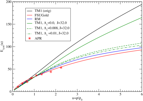
Figure 1: The density dependence of the symmetry energy for nonlinear models. For comparison the results obtained for the ordinary TM1 parameter set has been included.

Vector mesons-hyperon coupling constants are taken from the quark model and they are given by relations (38). Whereas in the scalar sector the scalar coupling of the $\Lambda$ and $\Xi$ hyperons requires constraining in order to reproduce the estimated values of the potential felt by a single $\Lambda$ and a single $\Xi$ in the saturated nuclear matter. The analysis of the experimental data concerning the binding energies of $\Lambda$’s bound in single particle orbitals in hypernuclei over an extensive range of mass numbers makes it possible to determine the potential depth of a single $\Lambda$ in nuclear matter at the value of

$$U_{\Lambda}^{(N)}\simeq 27-30\,MeV$$ (102)

which corresponds to $\sim$ 1/2 of the nucleon well depth $U_{N}^{(N)}$. There is still considerable uncertainty about the experimental status of $\Sigma$-nucleus potential. The calculations of $\Sigma$ hypernuclei have been based on analysis of $\Sigma^{-}$ atomic data. Phenomenological analysis of level shifts and widths in $\Sigma^{-}$ atoms made by Batty et al. [52, 53] indicates that the $\Sigma$ potential is attractive only at the nuclear surface, becoming repulsive for increasing density. The small attractive component of this potential is not sufficient to form bound $\Sigma$-hypernuclei. Also according to recent experimental data it has been established that the $\Sigma$ nuclear interaction is strongly repulsive.
The following values of the potentials have been used [55]

$$U_{\Lambda}^{(N)}=-28MeV,\,\,U_{\Sigma}^{(N)}+30MeV,\,\,U_{\Xi}^{(N)}=-18MeV$$ (103)

for the determination of the $g_{\sigma\Lambda}$, $g_{\sigma\Sigma}$ and $g_{\sigma\Lambda}$ coupling constants. In order to properly describe hyperon rich neutron star matter, the knowledge of the hyperon-hyperon interaction is indispensable. Data on $\Lambda\Lambda$ hypernuclei are scarce. Observation of double-strange hypernuclei $\Lambda\Lambda$ provide information about the $\Lambda-\Lambda$ interaction. Several events have been identified which indicate an attractive $\Lambda\Lambda$ interaction. The analysis of the data allows one to estimate the binding energies of ${}_{\Lambda\Lambda}^{6}$He, ${}_{\Lambda\Lambda}^{10}$Be and ${}_{\Lambda\Lambda}^{13}$B. The interaction between other type of hyperons are not known experimentally [54, 56]. The hyperon couplings to strange meson $\sigma^{\ast}$ have been obtained from the following relations

$$U_{\Xi}^{(\Xi)}\simeq U_{\Lambda}^{(\Xi)}\simeq 2U_{\Xi}^{(\Lambda)}\simeq 2U_{\Lambda}^{(\Lambda)}.$$ (104)

In summery the coupling of hyperons to the strange meson $\sigma^{\ast}$ has been limited by the estimated value of hyperon potential depths in hyperon matter this has also direct consequences for neutron star parameters. Recent experimental data [42] indicate a much weaker strength of hyperon-hyperon interaction. The currently obtained value of the $U_{\Lambda}^{(\Lambda)}$ potential at the level of 5 MeV permits the existence of the additional parameter set which reproduces this weaker $\Lambda\Lambda$ interaction. The parametrisation considered in this paper includes for comparison the strong and weak hyperon-hyperon couplings. The strong $Y-Y$ interaction is related to the value of the potential $U_{\Lambda}^{(\Lambda)}=-20$ MeV, whereas the weak one corresponds to $U_{\Lambda}^{(\Lambda)}=-5$ MeV [42], [43].
The inclusion of additional parameters in the isovector meson sector requires the adjustment of the $g_{\rho N}$ parameters. The new values of parameters are collected in Table 6.

Y–Y interaction	$g_{\sigma\Lambda}$	$g_{\sigma\Xi}$	$g_{\sigma^{\ast}\Lambda}$	$g_{\sigma^{\ast}\Xi}$
weak	6.17	2.202	5.41	11.516
strong	6.17	3.202	7.018	12.6

Table 5: Strange scalar sector parameters

	$\Lambda_{V}=0$	$\Lambda_{V}=0.008$	$\Lambda_{V}=0.01$
$g_{\rho N}$	9.2644	10.207	10.4828

Table 6: The $g_{\rho N}$ parameters for different values of the parameter $\Lambda_{V}$

7 Results

Having obtained the EOS that relates the energy density and pressure the corresponding solution of the Tolman-Oppenheimer-Volkoff (TOV) equations can be found and estimation of neutron star masses and radii become possible. The EOS and especially its high density limit has inevitable consequences for neutron star parameters. This manifests itself in a deep sensitivity of neutron star masses and radii to the stiffness of the EOS and allows one to study the influence of nonlinear vector meson interaction terms on neutron star properties.

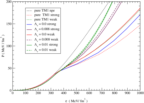
Figure 2: The EOS obtained for the nonlinear models. The limiting cases of the EOS indicate that the stiffest one has been obtained for the non-strange matter, whereas the softest represents the case of the standard TM1 model extended by the inclusion of strange mesons which have been introduced in a minimal fashion. The remaining EOS for the nonlinear models with different values of the parameter $\Lambda_{V}$ are located between these two curves.

The integration of the TOV equations with a specific equation of state leads to the mass-radius relation and allows one to determine the value of the maximum mass which in a sense can give a measure of the impact of particular nonlinear couplings between vector mesons. In Fig. 2 the equations of state obtained for different cases of nonlinear potentials presented in this paper have been shown. Extreme, dashed curves represent results obtained for the standard TM1 parameterisation, for the non-strange and strangeness rich matter respectively. The case when the matter includes only nucleons and leptons gives the stiffest EOS whereas the directly opposed result namely the softest EOS can be obtained for the standard TM1 parameterisation extended by the inclusion of hyperons. The vector meson sector in this case comprises the quartic vector meson $\omega_{\mu}$ self-interaction term supplemented by the linear term for the hidden-strange meson $\phi_{\mu}$. The influence of the strength of hyperon-hyperon interaction is also illustrated by comparing equations of state calculated for the weak and strong $Y-Y$ interaction. Other equations of state presented in this figure aim to provide the analysis of the influence of additional vector meson nonlinear interaction. Relating this problem to the introduced scheme for nonlinear potentials, the consider cases $\Lambda_{V}=0.008$ and $\Lambda_{V}=0.01$ are taking into account. The obtained results indicate for the strong tendency for stiffening of the EOS for the increasing value of the parameter $\Lambda_{V}$, approaching the limiting case for $\Lambda_{V}=0.01$. Moreover, there exists evidence for diminishing the differences between the weak and strong $Y-Y$ interaction for increasing value of the parameter $\Lambda_{V}$. Calculations performed for the value of the parameter $\Lambda_{V}>0.01$ lead to acausal behavior of the equation of state at high density.
The inclusion of nonlinear vector meson interactions has profound consequences for the structure of neutron stars and this can be deduced from Fig. 3 where the mass-radius relations for the obtained equations of state have been shown. Dotted curves depicts the results calculated for non-strange matter. Arrows marked by $\beta=0$ and $\beta=1$ denotes the solutions obtained for ordinary TM1 parameter set and for the TM1 supplemented by the nonlinear $\omega-\rho$ coupling between the isoscalar and the isovector mesons. In the case of strangeness rich matter the results for different values of the parameter $\Lambda_{V}$ has been included. The arrow marked $\Lambda_{V}$ shows the influence of the nonlinear terms on neutron star parameters especially for radii. For comparison the mass-radius relation for the FSU Gold parameter set has been given. This figure depicts also constraints obtained from Vela and XTEJ 11739-285 data [58].

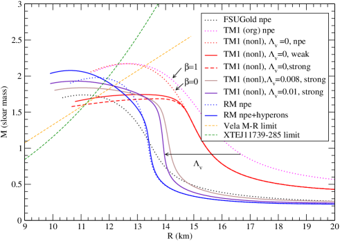
Figure 3: The mass-radius relations obtained for the chosen models.

Fig 4 depicts models obtained for the value of $\Lambda_{V}=0.008$ with and without the nonhomogenous inner crust phase. This figure compares the solutions obtained for different structure of the outer layer of the neutron star. The presented results includes the homogenous neutron star model without the crust which is represented by dotted curve whereas dashed and solid lines depicts the mass-radius relations for the crust without and with the nonhomogenous inner crust, respectively. For both cases the critical density $\rho_{t}$ is given. A comparison of Fig. 3 and Fig. 4 leads to the conclusion that results obtained for higher value of the parameter $\Lambda_{V}$ gives lower value of the critical density $\rho_{t}$ and as a consequence diminishes the nonhomogenous inner crust.

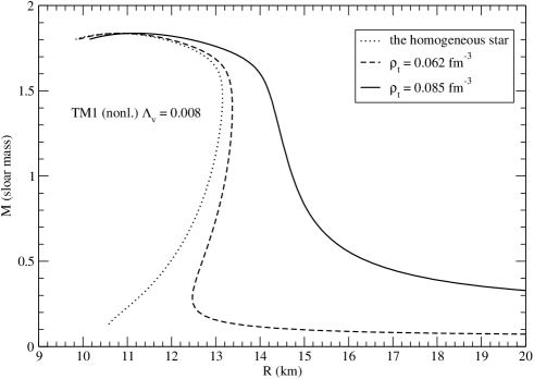
Figure 4: The mass-radius relation for the chosen models. It includes for comparison homogenous model without outer envelope.

The values of the maximum masses and the corresponding values of radii for the strangeness rich matter have been collected in Table 7. Results have been calculated for selected values of the parameter $\Lambda_{V}$.

$\Lambda_{V}$	$\rho_{max}(gcm^{-3})$	$M_{\max}(M_{\odot})$	$R(M_{\max})$
$\Lambda_{V}=0$	14.4	1.62	12.92
$\Lambda_{V}=0.008$	27.4	1.95	10.53
$\Lambda_{V}=0.01$	28.7	2.161	10.06

Table 7: The value of the maximum mass configurations and the corresponding radii for different values of the parameter $\Lambda_{V}$

The maximum mass increases with increasing value of the parameter $\Lambda_{V}$, given in the results neutron star models with masses exceeding $2M_{\odot}$ and with reduced radii. Thus, one can expect that solutions with nonlinear vector meson couplings lead to neutron star models with substantially greater density. The mass-radius diagrams have been obtained for variety of models presented in this paper. It includes the cases for non-strange and strange matter. Firstly solution for the pure TM1 model only with quartic $\omega$ term is compared with the enlarged nonlinear TM1 one which additionally comprises quartic $\rho$ meson term. From these two mass-radius relations it is evident that the presence of the quartic $\rho$ meson term influences mainly neutron star radii. Changing the value of the parameter $\Lambda_{V}$ solutions with substantially reduced value of the transition density is obtained. This points to the conclusion that the crust-core boundary moves to lower density region leading to the models with reduced value of non-homogenous phase. This is confirmed in Fig. 5 which shows the density profile of neutron star matter for maximum mass configuration. Models with nonlinear vector meson couplings give as a result neutron stars with densities much more higher than that obtained for the case $\Lambda_{V}=0$.

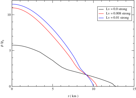
Figure 5: The density profiles in the models representing the maximum mass configurations.

The analysis of the density profiles indicates for the existence of different regions in neutron star interiors. These regions corresponds to the envelope and the core. In the core there is distinct part, with substantially increased density. This is connected with the appearance of strange matter. In the case of nonlinear models the inner core with nonzero strangeness spread through-out almost the whole star leading to very uniform neutron star model with considerably reduced outer parts.
The appearance of hyperons follows from the chemical potential relations. It has been shown that the composition of hyperon star matter as well as the threshold density for hyperons, is altered when the strength of the hyperon-hyperon interaction is changed.

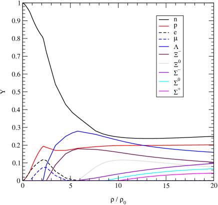
Figure 6: Relative concentrations of baryons for the model with $\Lambda_{V}=0$, for the strong $Y-Y$ interaction.

However, the inclusion of nonlinear vector meson interactions also significantly modifies the chemical composition of the star. In order to get more complete understanding of the influence of nonlinear vector meson coupling on particular baryon and lepton concentration it is interesting to analyze this issue from different perspectives.

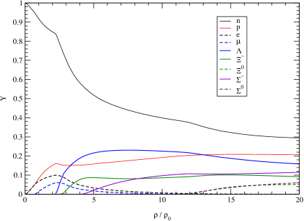
Figure 7: Relative concentrations of baryons for the model with nonlinear vector coupling for $\Lambda_{V}=0.008$, for the strong $Y-Y$ interaction.

Fig. 6 and 7 show relative fractions of particular baryon species $YB_{i}$ ($i=n,p,\Lambda,\Xi^{-},\Xi^{0},\Sigma^{-},\Sigma^{+}$ and $\Sigma^{0}$) as a function of baryon number density $n_{b}$ for the strong value of $Y-Y$ interaction. Fig. 6 is constructed for the model without nonlinear vector meson coupling whereas Fig. 7 for the nonlinear model with $\Lambda_{V}=0.008$. All calculations have been done under the assumption that the repulsive $\Sigma$ interaction shifts the onset points of $\Sigma$ hyperons to very high densities.
$\Lambda$ is the first strange baryon that emerges in hyperon star matter, it is followed by $\Xi^{-}$ and $\Xi^{0}$ and $\Sigma$ hyperons. These figures show differences in baryon fractions but these differences are more clearly visible in Fig. 8 and 9 presenting $\Lambda$ and $\Xi$ hyperon concentrations for different models.

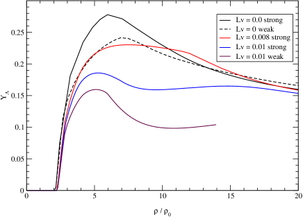
Figure 8: Concentrations of $\Lambda$ hyperons for the cases discussed in the text, for different values of the parameter $\Lambda_{V}$. For comparison the results obtained for the weak hyperon-hyperon interaction is also included. The weak models are constructed for $\Lambda_{V}=0$ and $\Lambda_{V}=0.008$.

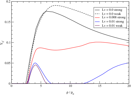
Figure 9: Concentrations of $\Xi^{-}$ hyperons for the cases discussed in the text, for different values of the parameter $\Lambda_{V}$. For comparison the results obtained for the weak hyperon-hyperon interaction is also included. The weak models are constructed for $\Lambda_{V}=0$ and $\Lambda_{V}=0.008$.

Fig. 8 and 9 depict the analysis done for several models focusing on comparing the results for different values of the parameter $\Lambda_{V}$. Generally the appearance of nonlinear vector meson interaction terms lowers the concentration of hyperons in neutron star matter. Thus there is a substantial reduction of the $\Lambda$ and $\Xi^{-}$ hyperon populations for the increasing value of $\Lambda_{V}$. In the case of $\Xi$ hyperon there is a density range for which the population of $\Xi$ hyperons vanishes. This results from the chemical equilibrium conditions which are set by relations among chemical potentials of the constituents of the neutron star matter. Chemical potentials depend on the effective baryon masses which have been substantially modified in the considered nonlinear models. For comparison the analysis of the influence of the hyperon-hyperon interaction strength has been included. Dashed lines in presented figures represent the concentrations of baryons for the weak $Y-Y$ interaction.
In Fig. 10 and 11 the analysis of the chemical composition of the star is depicted. These figures show profiles of particular baryon and lepton species as a function of the star radius. One can see that in the case of nonlinear models the hyperon core spreads through-out almost the whole interior of the star, however, it includes reduced population of hyperons. It is especially visible in the case os $\Xi^{-}$ hyperons. For the case $\Lambda_{V}=0.01$, there is no $\Xi^{-}$ hyperons in the core. This fact ic strictly connected with the population of leptons, and especially influences the population of muons.

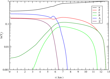
Figure 10: Baryon concentrations as a function of stellar radius for $\Lambda_{V}=0$.

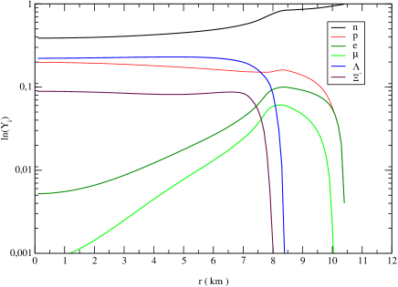
Figure 11: Baryon concentrations as a function of stellar radius for $\Lambda_{V}=0.008$

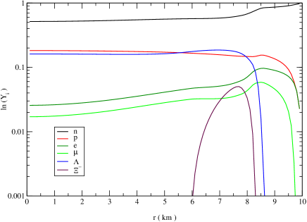
Figure 12: Baryon concentrations as a function of stellar radius for $\Lambda_{V}=0.01$

From the presented figures it is evident that lepton populations are altered not only by the change of strength of hyperon coupling constants but also by the isospin dependent nonlinearities which in turn determine the symmetry energy of the system. Thus a very special aspect of the existence of hyperons is the intrinsic deleptonization of neutron star matter. First the appearance of $\Lambda$ hyperons stops the increase in the lepton population and additionally when negatively charged $\Xi^{-}$ hyperons emerge further deleptonization occurs. Thus the charge neutrality can be guaranteed with the reduced lepton contribution. On the contrary in the hyperon core of of the nonlinear models when negatively charged $\Xi^{-}$ hyperons disappear lepton concentrations is substantially enhanced, and large population of muons establishes.

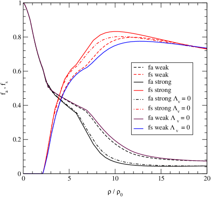
Figure 13: The asymmetry parameter $f_{a}$ and the strangeness fraction $f_{s}$ for models with $\Lambda_{V}=0$ as a function of the baryon number density.

Figure 14: The asymmetry parameter $f_{a}$ and the strangeness fraction $f_{s}$ for nonlinear models as a function of baryon number density.

In Fig 13 and 14 the density dependence of the asymmetry parameter $f_{a}=(n_{n}-n_{p})/(n_{b})$ which describes the relative neutron excess and the strangeness content $f_{s}$, defined as $(n_{\Lambda}+2n_{\Xi^{-}}+2n_{\Xi^{0}})/n_{B}$ are presented. Fig. 13 is constructed for the TM 1 parameter set supplemented by the strange sector and for the case when the coupling $\Lambda_{V}=0$. The second figure depicts the differences in the $f_{a}$ and $f_{s}$ behavior for two values of the $\Lambda_{V}$ coupling. In the case that no nonlinearities are included the parameter $f_{s}$ takes the maximal value. Next the nonlinearities have been added with the result that the strangeness content of the system is reduced. The increase of the $\Lambda_{V}$ parameter leads to even lower value of the strangeness fraction. The comparison of these two figure leads to the conclusion that the nonlinear model include matter more asymmetric but with lower value of the strangeness content.

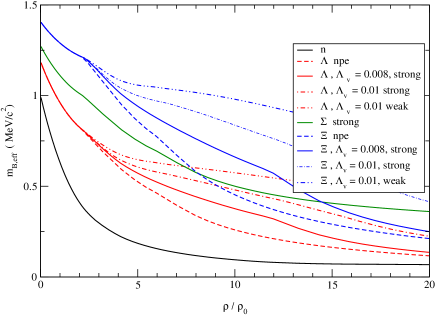
Figure 15: The effective baryon masses for different value of the parameter $\Lambda_{V}$ as a function of baryon number density.

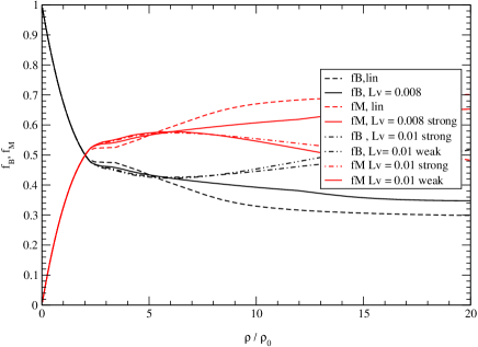
Figure 16: The fraction of baryon and meson contribution in the total energy of the system. Calculations have been done for linear and nonlinear mdels.

Fig. 15 presents changes of the effective baryon masses in dependance of the baryon density. It is common feature of the models that the effective baryon masses decreases with the increasing density. Very important aspects of the inclusion of nonlinear terms is connected with change of the effective baryon masses. In general the effective baryon masses are functions of $s_{0}$ and $s_{0}^{\ast}$. The numerical calculations show that the inclusion of nonlinear terms leads to the increase of the effective masses. Analysis has been done in comparison to the case when no nonlinearites are included.
In Fig. 16 the contributions of mesonic and baryonic parts to the total energy density is depicted. For the increasing density the nonlinear models lead to the situation when baryons and mesons give equal contributions to the energy of the whole system.

8 Conclusions.

Detailed knowledge about isospin asymmetric nuclear matter is of fundamental importance for understanding the structure of a neutron star, whose formation is preceded by the phenomenon of supernova explosion. In this paper a special class of the equations of state of asymmetric nuclear matter with non-zero strangeness have been analyzed in a systematic approach within the relativistic mean field model. The basic characteristic of the considered equations of state is the extended vector meson sector of the theory. This results in the appearance of various nonlinear vector meson couplings, among which there are terms which relate the strange and non-strange mesons. As a consequence strong connections between the asymmetry and strangeness fraction of the model have emerged. In order to construct neutron star models for the obtained equations of state the parameter sets which stem from the effective field theory and chiral SU(3) theory have been used. It has been shown that neutron star properties and through the properties also the neutron star structure are significantly affected not only by the presence of hyperons but also by the strength of hyperon-nucleon and hyperon-hyperon interactions. The results of the analysis performed for the nonlinear models have been compared with those obtained with the use of the standard TM1 parameter set extended by nonlinear meson interaction terms, which have been added for detailed investigations of the high density symmetry energy. It has been shown that in the very nonlinear models the inclusion of hyperons does not soften the EOS; on the contrary it leads to its considerable stiffening. The consequences for neutron star parameters are straightforward and appear as a considerable growth of neutron star masses. Thus one of the inevitable conclusions is that in the case of nonlinear models the inclusion of hyperons does not results in the lowering of a neutron star mass. This is of special interest when considering pulsar data reported which indicate large neutron star masses and radii. This refers to measurements of the neutron star mass in pulsar-white dwarf system. The analysis performed clearly indicates that also the structure of a neutron star is changed in the case of nonlinear models. Stars become more uniform and more compact. The threshold for the appearance of hyperons is shifted to the very outer part of the neutron star core, but in general the hyperon fraction is reduced when compared with the linear models. The reduction of the hyperon population in neutron star matter is related to the lepton concentrations. The models show that for a sufficiently large value of the parameter $\Lambda_{V}$ there are no $\Xi^{-}$ hyperons in the innermost part of the neutron star. Such particular models of the neutron star core reveal a hyperon reach layer with $\Lambda$ and $\Xi^{-}$ hyperons and the central region in which $\Xi^{-}$ hyperons vanish. In the latter case the populations of leptons and especially muons get enhanced.
The models analyzed include different types of nonlinear vector meson couplings. The additional coupling constants, which appear in these models are specified by the value of the parameter $\Lambda_{V}$ which is constrained by the requirement of causality for neutron star matter. The value of $\Lambda_{V}$ has profound influence on neutron star parameters. This is shown by Fig. 17 which depicts the dependance of the redshift $z$ on the value of the parameter $\Lambda_{V}$. The presented models can be compare with those which do not include nonlinear vector meson interactions [59], these solutions lead to very particular form of EOS This very particular form of the EOS generate different solutions of the Oppenheimer-Tolman-Volkoff equations. In the case of the cold neutron star model, apart from the ordinary neutron star branch, there exists an additional stable branch of solutions.

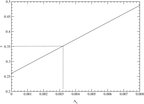
Figure 17: The dependance of the redshift $z$ on the value of the parameter $\Lambda_{V}$

The detection of redshifted O and Fe lines by XMM-Newton from the surface of the neutron star EXO 0748-676 [37] indicates for rather stiff EOS.

References

References

• [1] N.K. Glendenning, Astrophys.J. 293, 470 (1985); Compact Stars, Sringer-Verlag, New York (1997)
• [2] I. Bednarek, R. Manka, Int.Journal Mod.Phys. D10, 607 (2001)
• [3] F. Weber, Pulsars as Astrophysical Laboratories for Nuclear and Particle Physics, IOP Publishing, Philadelphia (1999)
• [4] J. Schaffner-Bielich and A. Gal, Phys. Rev. C62, 034311 (1999)
• [5] C.J. Pethic and D.G. Ravenhall, Annu. Rev. Nucl. Part. Phys. 45, 429 (1995)
• [6] I.E. Lagaris and V.R. Pandharipande, Nucl. Phys. A369, 470 (1981)
• [7] R. B. Wiringa, V. Fiks, and A. Fabrocini, Phys. Rev. C38, 1010 (1988)
• [8] W. Zuo, A. Lejeune, U. Lombardo, and J.F. Mathiot, Nucl. Phys. A706, 418 (2002)
• [9] I. Bombaci, U. Lombardo, Phys. Rev. C44, 1892 (1991)
• [10] H.Q. Song, Z.X. Wang, and T.T.S. Kuo, Phys. Rev. C46, 1788 (1992)
• [11] G.Q. Li, R. Machleidt, and R. Brockmann, Phys. Rev. 45, 2782 (1992)
• [12] ENE. van Dalen, C. Fuchs, and A. Faessler, Phys. Rev. Lett. 95, 022302 (2005)
• [13] T. Klahn, et al. Phys. Lett. B654, 170 (2007)
• [14] P. Danielewicz, R. Lacey, and W.G. Lynch, Science 298, 1592 (2002)
• [15] G. Stoicea, et al., FOPI Collaboration, Phys. Rev. Lett. 92, 072303 (2004)
• [16] C. Fuchs,Prog. Part. Nucl. Phys. 56, 1 (2006)
• [17] B.D. Serot and J.D. Walecka, Adv. Nucl. Phys. 16, 1 (1986); B.D. Serot and J.D. Walecka, Int. J. Mod. Phys. E6, 515 (1997)
• [18] D.H. Youngblood, C.M. Rozsa, J.M. Moss, D.R. Brown, and J.D. Bronson, Phys. Rev. Lett. 39, 1188 (1977)
• [19] J. Boguta and A.R. Bodmer, Nucl. Phys. A292, 413 (1977); Int. J. Mod. Phys. E6, 515
• [20] A.R. Bodmer, Nucl. Phys. A526, 703 (1991)
• [21] G. Colo, N. Van Giai, J. Meyer, K. Bennaceur, and P. Bonche, Phys. Rev. Lett. 91, 050401 (2003)
• [22] U. Garg et al., Nucl. Phys. A788, 36 (2007)
• [23] J. Piekarewicz, Phys. Rev. C76,064310 (2007)
• [24] Lie-Wen Chen, Che Ming Ko, and Bao-An Li, Phys. Rev. C76, 054316 (2007)
• [25] Y. Sugahara and H. Toki, Prog. Theo. Phys 92, 803 (1994)
• [26] R. J. Furnstahl, Nucl. Phys. A706, 85 (2002)
• [27] A.W. Steiner, M. Prakash, J.M. Lattimer, and P.J. Ellis, Phys. Rept. 411, 325 (2005)
• [28] C.J. Horowitz and J. Piekarewicz, Phys. Rev. Lett. 86, 5647 (2001)
• [29] B.G. Todd-Rutel and J. Piekarewicz, Phys. Rev. Lett. 95, 122501 (2005)
• [30] P. Papazoglou, D. Zschiesche, S. Schramm, J. Schaffner-Bielich, Ch. StΓΆcker, and W. Greiner, Phys. Rev. C59, 411 (1998); P. Papazoglou, S. Schramm, J. Schaffner-Bielich, Ch. StΓΆcker, and W. Greiner, 1998, Phys. Rev., C57, 2576 (1998); M. Hanauske, D. Zschiesche, S. Pal, S. Schramm, Ch. StΓΆcker, and W. Greiner, 2000, Aatrophys. J. 573, 958 (2000)
• [31] I. Sagert, M. Wietoska, J. Schaffner- Bielich, and Ch. Sturm, J. Phys. G35, 014053 (2008)
• [32] D. J. Nice, E.M. Splaver, I.H. Stairs, O. Lohmer, A. Jessner, M. Kramer, and J.M. Cordes, Astrophys. J. 634, 1242 (2005)
• [33] Conference contribution by D. Nice, 40 Years of Pulsars, Montreal, 2007
• [34] J.E. TrΓΌmper, V. Burvitz, F. Haberl, and V.E. Zavlin, Nucl. Phys. (proc. Suppl.) B132, 560 (2004)
• [35] D. Barret, J.F. Olive, and M.C. Miller, Mon. Not. R. Astron. Soc. 361, 855 (2005)
• [36] J. Cottam, F. Paerles, and M. Mendez, Nature 420, 51 (2002)
• [37] F. Γ–zel, Nature 441, 1115 (2006)
• [38] —–, Int.J.Mod.Phys E6, 51 (1997)
• [39] J. Schaffner, C.B. Dover, A. Gal, C. Greiner, D.J. Millner, and H. Stocker, Ann.Phys. 235, 35 (1994)
• [40] H. Muller and B.D. Serot, Nucl. Phys. A606, 508 (1996)
• [41] C.J. Horowitz, and J. Piekarewicz, Phys. Rev. C64, 064616 (2001)
• [42] Takahashi et al. Phys. Rev. Lett. 87 212502 (2001)
• [43] H.Q. Song, R.K. Su, D.H. Ku, and W.L. Qian, Phys. Rev. C68, 055201 (2003)
• [44] Jun Xu, Lie-Wen Chen, Bao - An Li, and Hong-Ru Ma, arXiv:0901.2309 (2009)
• [45] Jun Xu, Lie-Wen Chen, Bao-An Li, and Hong-Ru Ma, Phys. Rev. C79, 035802, (2009)
• [46] K.C. Chung, C. S. Wang, A.J. Santiago, and J.W. Zhang, Phys. Rev. C61, 047303 (2000)
• [47] Bao-An Li, L.W. Chen, and C.M. Ko, Phys. Rep. 464, 113 (2008).
• [48] J. Piekarewicz and M . Centelles, arXiv:0812.4499, (2008)
• [49] M. Centelles, X. Roca-Maza, X. Vinas, and M. Warda, Phys. Rev. Lett. 102, 122502, (2009)
• [50] R. Manka and I. Bednarek, J. Phys. G27 (2001)
• [51] A. Akmal, V.R. Pandharipande, and D.G. Ravenhall, Phys. Rev. C58, 1804 (1998)
• [52] C.J. Batty, E. Friedman, A. Gal, and B.K. Jennings, Phys. Lett. 335, 273 (1994)
• [53] E. Friedman and A. Gal, Phys. Rept. 452, 89 (2007)
• [54] J . Schaffner, and I.N. Mishustin, Phys. Rev. C53,1416 (1996)
• [55] J. Schaffner-Bielich, M. Hanauske , H. Stocker, and W. Greiner, Phys. Rev. Lett. 89, 171101 (2002)
• [56] J. Schaffner- Bielich, arXiv:0801.3791 (2008)
• [57] Lie-Wen Chen, Che Ming Ko, and Bao-An Li, Phys. Rev. C76, 054316 (2007)
• [58] Bao-An Li, Lie-Wen Chen, Che Ming Ko, Plamen G. Krastev, De-Hua Wen, Aaron Worley, Zhigang Xiao, Jun Xu, Gao-Chan Yong, and Ming Zhang, arXiv:0902.3284 (2009)
• [59] A. Bhattacharyya, S. K. Ghosh, M. Hanauske, and S. Raha, Astron. Astrophys. 418, 795 (2004)