A family of mixed finite element pairs with optimal geostrophic balance

Abstract

We introduce a family of mixed finite element pairs for use on geodesic grids and with adaptive mesh refinement for numerical weather prediction and ocean modelling. We prove that when these finite element pairs are applied to the linear rotating shallow water equations, the geostrophically balanced states are exactly steady, which means that the numerical schemes do not introduce any spurious inertia-gravity waves; this makes these finite element pairs in some sense optimal for numerical weather prediction and ocean modelling applications. We further prove that these finite element pairs satisfy an inf-sup condition which means that they are free of spurious pressure modes which would pollute the numerical solution over the timescales required for large-scale geophysical applications. We then discuss the extension to incompressible Euler-Boussinesq equations with rotation, and show that for the linearised equations the balanced states are again exactly steady on arbitrary unstructured meshes. We also show that the discrete pressure Poisson equation resulting from these discretisations satisfies an optimal stencil property. All these properties make the discretisations in this family excellent candidates for numerical weather prediction and large-scale ocean modelling applications when unstructured grids are required.

1 Introduction

The aim of this paper is to introduce a new family of finite element pairs for discretising large-scale ocean and atmosphere flows, state theorems about their wave propagation properties, and to explain why these properties are important for numerical weather prediction and ocean modelling. Section 1.1 provides some motivational background, section 1.2 describes the balance properties of model equations that we aim to preserve exactly in the numerical discretisations, and section 1.3 explains how these properties can be modified by numerical discretisations. Section 2 introduces the family of finite element pairs, and the optimal balance property is proved in section 3. It is also shown, by proving an inf-sup condition, that the finite element pairs are free from spurious pressure modes. In section 4 these properties are extended to the case of three-dimensional rotating stratified incompressible flow which applies to non-hydrostatic ocean modelling. Finally, section 5 provides a summary and outlook to future developments.

1.1 Background

An operational weather forecasting system combines observational data (such as satellite images, and pressure measurements on the Earth’s surface, for example) with a numerical model of the atmosphere (solved on state-of-the-art parallel computers) to produce weather forecasts. The numerical model consists of a mathematically-consistent discretisation of the equations of motion for the atmosphere (known as the dynamic core) together with schemes (known as parameterisations) for representing subgrid scale physics such as convection and turbulence, and physical processes such as cloud formation and atmospheric chemistry. Most current state-of-the art numerical weather prediction (NWP) models, such as the MET Office Unified Model [7], make use of a latitude-longitude grid to construct the numerical approximations to the fluid dynamical equations that form the dynamical core of the model. However, recently there has been growing interest in more general horizontal discretisation schemes constructed using triangles or hexagons. This is for two reasons. Firstly, geodesic grids (which are obtained by iterative refinement of an icosahedron using triangles or the dual grid which comprises a combination of hexagons plus exactly 12 pentagons) provide a much more uniform coverage over the sphere, which has possible advantages for accurate representation of wave propagation and avoids very fine grid cells near to the North and South poles. A number of groups are now using geodesic grids for weather and climate models [20, 14, 22]. Secondly, triangles facilitate adaptive mesh refinement much more easily, allowing regional models to be nested seamlessly in a global model, and even allowing dynamic mesh refinement in which the mesh is dynamically adapted during a forecast. However, the introduction of adaptively-refined triangular grids calls for the careful design of new numerical schemes which correctly represent the large scale geophysical balances so that model forecasts can be run over sufficiently long times (the current forecast window is about a week). In this paper we introduce a new family of numerical discretisation methods on triangular grids which shall be shown to optimally represent these geophysical balances on arbitrary unstructured grids. We also extend these properties to three dimensional rotating stratified incompressible flow so that they may be applied to non-hydrostatic ocean modelling.

1.2 Model equations and geostrophic states

As a model problem, we consider the shallow-water equations on an $f$-plane

$${\boldsymbol{u}}_{t}+({\boldsymbol{u}}\cdot\nabla){\boldsymbol{u}}+f{\boldsymbol{u}}^{\perp}+g\nabla D = 0,\quad{\boldsymbol{u}}=(u_{1},u_{2}),\quad{\boldsymbol{u}}^{\perp}=(-u_{2},u_{1}),$$ (1)

$$\quad D_{t}+\nabla\cdot({\boldsymbol{u}}D) = 0,$$ (2)

where ${\boldsymbol{u}}$ is the horizontal velocity, $D=\bar{D}+\eta$ is the total layer depth, $\eta$ is the perturbation layer thickness, $\bar{D}$ is the mean layer thickness, ${\boldsymbol{k}}$ is the unit vector in the $z$-direction, $f$ is the (constant) Coriolis parameter and $g$ is the acceleration due to gravity. The boundary conditions are

$${\boldsymbol{u}}\cdot{\boldsymbol{n}}=0\quad\mathrm{on}\quad\partial\Omega,$$ (3)

where $\partial\Omega$ denotes the boundary of the two-dimensional domain $\Omega$, and ${\boldsymbol{n}}$ is the normal to $\partial\Omega$. These equations model the dynamics of a layer of hydrostatic incompressible fluid with constant density with a free surface and columnar motion so that the horizontal velocity is independent of depth. This can be thought of as a simple model for the ocean, or for a single layer in the atmosphere. For a derivation of these equations, see [21], for example. Numerical methods for NWP and ocean modelling are often developed in two dimensions using the rotating shallow-water equations. The methods can then be extended to the primitive equations (three-dimensional equations of rotating stratified hydrostatic flow, see [21]) by building a mesh in layers in which the two-dimensional discretisation is applied in the horizontal plane. Hence, the shallow-water equations provide a useful testbed for numerical schemes and a stepping stone to the primitive equations which already poses many of the key challenges for designing good numerical methods for NWP and ocean modelling.

A key dimensionless number in geophysical fluid dynamics is the Rossby number, defined by

$$\operatorname{Ro}=U/fL,$$

where $U$ is a typical velocity scale, and $L$ is a typical horizontal length scale; the Rossby number measures the relative importance of the acceleration and Coriolis terms. Geophysical flow problems in the small Rossby number limit are concerned with the states which satisfy

$$f{\boldsymbol{u}}^{\perp}+g\nabla D\approx 0$$

so that the Coriolis term approximately balances the pressure gradient. This is the state of geostrophic balance. It has long been observed (see [15, 16], for example) that if the initial conditions for the state variables ${\boldsymbol{u}}_{0}({\boldsymbol{x}})$ and $D_{0}({\boldsymbol{x}})$ are initialised near to geostrophic balance, then this state will be approximately preserved for very long times. This has observed to be the case both in the low Rossby number limit, and also in the $\mathcal{O}(1)$ limit and various mechanisms have been proposed for the maintenance and breakdown of this balance in various parameter regimes [9, 6, 17]). Large scale flows in the atmosphere and ocean (such as those associated with the global circulation that determines global weather and climate) are observed to be in a state of geostrophic balance and hence it is important that numerical schemes used for weather forecasting, ocean modelling and climate prediction can correctly represent these balances.

The ability of a numerical scheme to represent geostrophic balance can be examined by studying wave propagation properties. Choosing a flat topography so that $\bar{D}$ is a constant, the linearised shallow-water equations are

$${\boldsymbol{u}}_{t}+f{\boldsymbol{u}}^{\perp}+g\nabla\eta = 0,$$ (4)

$$\quad\eta_{t}+\bar{D}\nabla\cdot{\boldsymbol{u}} = 0.$$ (5)

If the velocity ${\boldsymbol{u}}$ and free surface elevation $\eta$ are chosen in a state of perfect geostrophic balance so that

$$f{\boldsymbol{u}}^{\perp}+g\nabla\eta=0,$$

then the velocity divergence satisfies

$$\nabla\cdot{\boldsymbol{u}}=\frac{g}{f}\nabla\cdot\nabla^{\perp}\eta=-\eta_{yx}+\eta_{xy}=0,\qquad\nabla^{\perp}=(-\partial_{y},\partial_{x})$$

and so we have a steady state

$${\boldsymbol{u}}_{t}=0,\quad\eta_{t}=0.$$

Hence, all geostrophically-balanced states are steady for the linearised equations. In the nonlinear case, the solutions variables evolve through the nonlinear advection terms which are small in the low Rossby number limit, and hence the geostrophic balance is maintained as a form of adiabatic invariance due to the small parameter $\operatorname{Ro}$.

If periodic boundary conditions are chosen, then one can perform a dispersion analysis for solutions of equations (4-5) by substituting the ansatz

$${\boldsymbol{u}}=\hat{{\boldsymbol{u}}}e^{i\left({\boldsymbol{k}}\cdot{\boldsymbol{x}}-\omega t\right)},\qquad\eta=\hat{\eta}e^{i\left({\boldsymbol{k}}\cdot{\boldsymbol{x}}-\omega t\right)},$$

resulting in the dispersion relation

$$\omega\left(\omega^{2}-f^{2}-g\bar{D}\left(k^{2}+l^{2}\right)\right)=0.$$ (6)

This equation has three roots, with the $\omega=0$ root corresponding to the steady geostrophic state; this branch becomes the Rossby wave branch when the model is extended to the $\beta$-plane model in which the Coriolis parameter $f$ varies in the $y$-direction so that $f=f_{0}+\beta y$ for constants $f_{0}$ and $\beta$. The other two roots give rise to dispersive waves, known as inertia-gravity waves; the $k=l=0$ case is known as an inertial oscillation in which the fluid undergoes solid body motion with a flat free surface. Since all of the roots are real, the state of geostrophic balance is stable under small perturbations.

1.3 Geostrophic states for numerical methods

It is crucial that numerical methods for equations (1-2) do not generate spurious inertia-gravity waves when the solution is near to geostrophic balance. This can typically occur if the wave-propagation properties of the numerical method (i.e. the numerical discretisation of the linearised equations) do not correctly represent this balance. Given a discretisation of the linear system (4-5) it is simple to check the evolution of geostrophically-balanced states under this discretisation. One constructs initial conditions which satisfy the discrete form of geostrophic balance, steps the variables forward in time, and inspects the variables to check that the steady state is approximately preserved. This analysis has been performed for various element pairs in [13]. In general, the discrete divergence of the velocity field will not be exactly zero, and the remainder due to numerical discretisation errors will lead to oscillations. Whether the numerical method is suitable for computing the evolution of geostrophically-balanced states over long time intervals (i.e. suitable for weather forecasting or ocean modelling) depends on how these errors behave. If one computes the numerical dispersion relation (i.e. the numerical analogue of equation (6) for the method (see for example the calculations in [23, 12]) then it is possible to divide the eigenmodes of the system into geostrophic modes which converge to the geostrophic states as the mesh edge-lengths converge to zero, and inertia-gravity modes which converge to the inertia-gravity waves. If the numerical discretisation errors in the divergence of the balanced states are large and project onto the inertia-gravity modes, then large unbalanced dynamics will be apparent after a long time integration interval (such as the time interval that is relevant to weather forecasting). When solving the nonlinear equations these numerical errors are constantly generated by the nonlinear terms, resulting in the geostrophic component of the solution being polluted by spurious inertia-gravity waves which render the numerical scheme useless for NWP and global ocean modelling.

In section 2 we present a family of mixed finite element pairs which have the optimal property that the geostrophically balanced states are exactly steady; this means that these numerical discretisations are in some sense optimal for geophysical fluid dynamics problems. This property is independent of the choice of mesh, which can be taken to be completely unstructured. This means that the numerical discretisations can be used to solve geophysical flow problems in the presence of mesh refinement and adaptivity. This is proved in theorem 12 in section 3. We shall also show that the finite element pairs satisfy an inf-sup condition which means that they are free from spurious pressure modes: eigenmodes which have very small discrete gradients of free surface elevation despite having a free surface which is not flat. The absence of these modes is also crucial for geophysical applications since they can be coupled to the physical modes through the nonlinear terms and eventually becoming as large as the physical solution; the existence of these modes prohibits the use of such numerical methods in weather forecasting and ocean modelling. This result is proved in theorem 16, also in section 3. The proofs of these results are very simple and elegant, due to the geometric embedding conditions that define the family of discretisations.

2 Family of finite element pairs

In this section we introduce our family of finite element pairs, first by developing the general finite element formulation in section 2.1, and then by stating conditions which define our particular family in section 2.2.

2.1 Finite element formulation

In this subsection we develop the finite element approximation to the linearised shallow-water equations by writing down the weak form of the equations and restricting the function spaces to chosen spaces of piecewise polynomials on a finite element mesh. We start with the linearised shallow-water equations on an $f$-plane given in equations (4-5) with boundary conditions given by equation (3). To obtain the weak form of the equations we multiply equation (4) by a test function ${\boldsymbol{w}}$ and equation (5) by a test function $\phi$ and integrate over the domain $\Omega$ to obtain

$$\frac{\operatorname{d}}{\operatorname{d}t}\int_{\Omega}{\boldsymbol{w}}\cdot{\boldsymbol{u}}\operatorname{d}{V}+f\int_{\Omega}{\boldsymbol{w}}\cdot{\boldsymbol{u}}^{\perp}\operatorname{d}{V} = -g\int_{\Omega}{\boldsymbol{w}}\cdot\nabla\eta\operatorname{d}{V},$$ (7)

$$\frac{\operatorname{d}}{\operatorname{d}t}\int_{\Omega}\phi\eta\operatorname{d}{V} = -\bar{D}\int_{\Omega}\phi\nabla\cdot{\boldsymbol{u}}\operatorname{d}{V}.$$ (8)

We then integrate equation (8) by parts, and make use of the boundary conditions (3) to obtain

$$\frac{\operatorname{d}}{\operatorname{d}t}\int_{\Omega}{\boldsymbol{w}}\cdot{\boldsymbol{u}}\operatorname{d}{V}+f\int_{\Omega}{\boldsymbol{w}}\cdot{\boldsymbol{u}}^{\perp}\operatorname{d}{V} = -g\int_{\Omega}{\boldsymbol{w}}\cdot\nabla\eta\operatorname{d}{V},$$ (9)

$$\frac{\operatorname{d}}{\operatorname{d}t}\int_{\Omega}\phi\eta\operatorname{d}{V} = \bar{D}\int_{\Omega}\nabla\phi\cdot{\boldsymbol{u}}\operatorname{d}{V},$$ (10)

which must hold for all test functions ${\boldsymbol{w}}\in H^{1}(\Omega)$ and $\phi\in L_{2}(\Omega)$. This is the weak form of equations (4-5) which we shall discretise using the Galerkin finite element method.

The Galerkin projection of equations (9-10) is constructed by defining finite dimensional spaces for the numerical solution variables ${\boldsymbol{u}}^{\delta}$ and $\eta^{\delta}$, and the test functions ${\boldsymbol{w}}^{\delta}$ and $\phi^{\delta}$. We shall use a mixed finite element method (see [3] for an excellent general survey), which means that one type of finite element space shall be used for ${\boldsymbol{u}}^{\delta}$ and ${\boldsymbol{w}}^{\delta}$, and a different type of finite element space shall be used for $\eta^{\delta}$ and $\phi^{\delta}$.

We shall begin by defining the possible finite element spaces in general terms, before going on to state conditions which define our particular family of discretisations.

Definition 1 (Finite element mesh).

Let the mesh $\mathcal{M}$ be a set of non-overlapping polygons (elements) which completely cover the computational domain $\Omega$ which has a elementwise polygonal boundary $\partial\Omega$.

Definition 2 (Pressure space).

Let $H$ be a space of elementwise polynomials on $\mathcal{M}$, of type and continuity to be specified.

This is a general definition, but we note that we shall require at least $C^{0}$ continuity across element boundaries, since we apply gradients to $\phi^{\delta}$ and $\eta^{\delta}$ in equations (11-12).

Definition 3 (Velocity space).

Let $V$ be a space of vectors of elementwise polynomials on $\mathcal{M}$, of type and continuity to be specified (possibly differently to $H$).

We note that we do not require any continuity conditions for $V$, since gradients are not applied to ${\boldsymbol{u}}^{\delta}$ and ${\boldsymbol{w}}^{\delta}$ in equations (11-12).

Having defined $H$ and $V$, we may now write down the Galerkin finite element method for equations (4-5), which is obtained by restricting the solution variables and the test functions to these finite dimensional spaces.

Definition 4 (Galerkin finite element method).

${\boldsymbol{u}}^{\delta}({\boldsymbol{x}},t)$ and $\eta^{\delta}({\boldsymbol{x}},t)$ are the semi-discrete solutions of the Galerkin finite element discretisation of (4-5) if

$${\boldsymbol{u}}^{\delta}(\cdot,t)\in V,\quad\eta^{\delta}(\cdot,t)\in H,\qquad\forall t\in[0,T],$$

and

$$\frac{\operatorname{d}}{\operatorname{d}t}\int_{\Omega}{\boldsymbol{w}}^{\delta}\cdot{\boldsymbol{u}}^{\delta}\operatorname{d}{V}+f\int_{\Omega}{\boldsymbol{w}}^{\delta}\cdot{{\boldsymbol{u}}^{\delta}}^{\perp}\operatorname{d}{V} = -g\int_{\Omega}{\boldsymbol{w}}^{\delta}\cdot\nabla\eta^{\delta}\operatorname{d}{V},$$ (11)

$$\frac{\operatorname{d}}{\operatorname{d}t}\int_{\Omega}\phi^{\delta}\eta^{\delta}\operatorname{d}{V} = \bar{D}\int_{\Omega}\nabla\phi^{\delta}\cdot{\boldsymbol{u}}^{\delta}\operatorname{d}{V},$$ (12)

for all test functions ${\boldsymbol{w}}^{\delta}\in V$, $\phi^{\delta}\in H$.

This equations may be solved on a computer by expanding ${\boldsymbol{w}}^{\delta}$ and ${\boldsymbol{u}}^{\delta}$ in a basis for $V$, and $\phi^{\delta}$ and $h^{\delta}$ in a basis for $H$, which produces a matrix equation for the basis coefficients of ${\boldsymbol{u}}^{\delta}$ and $h^{\delta}$. This equation may then be discretised in time using a suitable time integration method.

2.2 Choice of finite element spaces

In defining the problem, it remains to select a particular choice spaces $(V,H)$ (known as a finite element pair). In this paper, we discuss a large family of possible choices defined by the following condition:

Definition 5 (Embedding conditions).

1. The operator $\nabla$ defined by the pointwise gradient

   $${q}^{\delta}({\boldsymbol{x}})=\nabla h^{\delta}({\boldsymbol{x}})$$

   maps from $H$ into $V$.

2. The skew operator $\perp$ defined by the pointwise formula

   $${\boldsymbol{q}}^{\delta}({\boldsymbol{x}})=({\boldsymbol{u}}^{\delta}({\boldsymbol{x}}))^{\perp}$$

   maps from $V$ into itself.

These conditions are most definitely not satisfied by all possible pairs $(V,H)$, as illustrated by the following examples.

Example 6 (P1-P1).

The finite element pair known as P1-P1 (which may be used for the shallow-water equations but requires stabilisation as described in [25]) is defined as follows:

• The mesh $\mathcal{M}$ is composed of triangular elements.

• $H$ is the space of elementwise-linear functions $h^{\delta}$ which are continuous across element boundaries.

• $V$ is the space of vector fields ${\boldsymbol{u}}^{\delta}$ with both of the Cartesian components $(u^{\delta},v^{\delta})$ in $H$.

Condition 1 of Definition 5 is not satisfied by the P1-P1 pair since gradients of functions in $H$ are discontinuous across element boundaries. Condition 2 is satisfied since the same continuity conditions are required for normal and tangential components.

Example 7 (RT0).

The lowest order Raviart-Thomas [19] velocity space (known as RT0) is constructed on a mesh $\mathcal{M}$ composed of triangular elements. It consists of elementwise constant vector fields which are constrained to have continuous normal components across element boundaries. RT0 does not satisfy condition 2 of Definition 5 since the $\perp$ operator transforms vector fields with discontinuities in the tangential component (which are permitted in RT0) into vector fields with discontinuities in the normal component (which are not).

We now describe some examples of finite element pairs which do satisfy the conditions in Definition 5.

Example 8 (P0-P1).

The finite element pair known as P0-P1 (applied to ocean modelling in [24], for example) is defined as follows:

• The mesh $\mathcal{M}$ is composed of triangular elements.

• $H$ is the space of elementwise-linear functions $h^{\delta}$ which are continuous across element boundaries.

• $V$ is the space of elementwise-constant vectors with discontinuities across element boundaries permitted.

Example 9 ($\textrm{P1}_{\textrm{DG}}$-P2).

The finite element pair known as $\textrm{P1}_{\textrm{DG}}$-P2 [5] is defined as follows:

• The mesh $\mathcal{M}$ is composed of triangular elements.

• $H$ is the space of elementwise-quadratic functions $h^{\delta}$ which are continuous across element boundaries.

• $V$ is the space of elementwise-linear vectors with discontinuities across element boundaries permitted.

Each of these examples satisfy both conditions in Definition 5: condition 1 holds because taking the gradient of a elementwise polynomial $n-1$ which is continuous across element boundaries results in a vector field which is discontinuous across element boundaries and is composed of elementwise polynomials of one degree $n$, and condition 2 holds since the velocity space uses the same continuity constraints for normal and tangential components e.g. both components are allowed to be discontinuous. This defines a whole sequence of high-order $\textrm{Pn}_{\textrm{DG}}$-P(n+1) element pairs. Similar elements can be constructed on quadrilateral elements. Since we only require these two conditions to prove our optimal balance property which holds on arbitrary meshes, we can also construct finite element spaces on mixed meshes composed of quadrilaterals and triangles, for example. It is also possible to use $p$-adaptivity in which different orders of polynomials are used in different elements, as long as the conditions are satisfied.

3 Geostrophic balance properties

In this section we prove that when finite element pairs which are chosen to satisfy both of the conditions in Definition 5, their discrete geostrophically-balanced velocities satisfy the discrete divergence-free condition exactly: this means that the discrete geostrophically-balanced states are exactly steady states of equations (11-12). This is the result of Theorem 12 in this section, which makes use of conditions 1 and 2 of Definition 5. We also prove an inf-sup condition for these finite element pairs (making use of condition 1 of Definition 5) which provides a lower bound (independent of edge-lengths in the mesh) for the discrete gradient operator applied to non-constant functions in $H$. This lower bound prohibits the existence of spurious pressure modes which render a finite element pair unsuitable for geophysical flow problems; it also allows one to prove the convergence of the numerical solutions at the optimal rate obtained from approximation theory. This condition is stated and proved in Theorem 16.

3.1 Optimal geostrophic balance

We first prove the following lemma which illustrates the embedding properties of our family of finite element pairs.

Lemma 10 (Pointwise gradient lemma).

Let $(H,V)$ be a finite element pair chosen to satisfy condition 1 in Definition 5. Let Let ${\boldsymbol{q}}^{\delta}\in V$ by the discrete gradient of $\eta^{\delta}\in H$ defined by

$$\int_{\Omega}{\boldsymbol{w}}^{\delta}\cdot{\boldsymbol{q}}^{\delta}\operatorname{d}{V}=\int_{\Omega}{\boldsymbol{w}}^{\delta}\cdot\nabla\eta^{\delta}\operatorname{d}{V},$$ (13)

for all test functions ${\boldsymbol{w}}^{\delta}\in V$. Then ${\boldsymbol{q}}^{\delta}$ is the pointwise (strong) gradient of $\eta^{\delta}$ defined by

$${\boldsymbol{q}}^{\delta}({\boldsymbol{x}})=\nabla\eta^{\delta}({\boldsymbol{x}}),\quad\forall{\boldsymbol{x}}\in\Omega.$$

Proof.

Since condition 1 is satisfied, we may choose a test function

$${\boldsymbol{w}}^{\delta}={\boldsymbol{q}}^{\delta}-\nabla\eta^{\delta}\in V,$$

and substitution into equation 13 gives

$$0 = \int_{\Omega}{\boldsymbol{w}}^{\delta}\cdot\left({\boldsymbol{q}}^{\delta}-\nabla\eta^{\delta}\right)\operatorname{d}{V}$$

$$= \int_{\Omega}\left|{\boldsymbol{q}}^{\delta}-\nabla\eta^{\delta}\right|^{2}\operatorname{d}{V}$$

$$= \|{\boldsymbol{q}}^{\delta}-\nabla\eta^{\delta}\|^{2}_{L_{2}}.$$

Since the $L_{2}$-norm only vanishes for elements of $H$ if they are identically zero, we conclude that ${\boldsymbol{q}}^{\delta}=\nabla\eta^{\delta}$ as required. ∎

This lemma appears at first sight to be a tautology but since the discrete gradient ${\boldsymbol{q}}^{\delta}$ can be thought of as the $L_{2}$-projection of $\nabla\eta^{\delta}$ into $V$, it requires condition 1 of Definition 5 to be satisfied, and it is not the case for equal-order element pairs such as P1-P1, for example. We shall make use of this lemma in proving Theorem 16.

The following lemma extends this technique to show that if the discrete geostrophic balance relation is satisfied by functions taken from a finite element pair in our family of discretisations, then the exact geostrophic balance condition is actually satisfied at each point.

Lemma 11 (Embedding lemma).

Let $(H,V)$ be a finite element pair chosen to satisfy both conditions in Definition 5. Let ${\boldsymbol{u}}^{\delta}\in V$ and $\eta^{\delta}\in H$ satisfy the discrete geostrophic balance relation

$$f\int_{\Omega}{\boldsymbol{w}}^{\delta}\cdot{{\boldsymbol{u}}^{\delta}}^{\perp}\operatorname{d}{V}=-g\int_{\Omega}{\boldsymbol{w}}^{\delta}\cdot\nabla\eta^{\delta}\operatorname{d}{V},$$ (14)

for all test functions ${\boldsymbol{w}}^{\delta}\in V$. Then

$$f({\boldsymbol{u}}^{\delta})^{\perp}({\boldsymbol{x}})=-g\nabla\eta^{\delta}({\boldsymbol{x}}),\quad\forall{\boldsymbol{x}}\in\Omega.$$ (15)

Proof.

Following the technique of the previous lemma, we note that conditions 1 and 2 mean that we may choose a test function

$${\boldsymbol{w}}^{\delta}=f{{\boldsymbol{u}}^{\delta}}^{\perp}+g\nabla\eta^{\delta}\in V,$$

and substitute into equation 14 to obtain

$$0 = \int_{\Omega}{\boldsymbol{w}}^{\delta}\cdot\left(f{{\boldsymbol{u}}^{\delta}}^{\perp}+g\nabla\eta^{\delta}\right)\operatorname{d}{V}$$

$$= \int_{\Omega}\left|f{{\boldsymbol{u}}^{\delta}}^{\perp}+g\nabla\eta^{\delta}\right|^{2}\operatorname{d}{V}$$

$$= \|f{{\boldsymbol{u}}^{\delta}}^{\perp}+g\nabla\eta^{\delta}\|^{2}_{L_{2}},$$

hence the result. ∎

This lemma is useful for initialising the system variables in a balanced state since the geostrophic balance relation can be evaluated pointwise instead of requiring a projection to be computed. Next we apply this lemma to prove the following theorem, which states that finite element pairs have the optimal property that these geostrophically balanced states are steady solutions of equations (11-12).

Theorem 12 (Steady geostrophic states).

Let ${\boldsymbol{u}}^{\delta}\in V$ and $\eta^{\delta}\in H$ satisfy equation (14), and let $\partial\Omega$ be a contour for $\eta^{\delta}$ (so that the balanced velocity field obtained from equation 15 satisfies the boundary condition). Then ${\boldsymbol{u}}^{\delta}$ and $\eta^{\delta}$ are steady solutions of equation (11-12).

Proof.

Substitution into equation (11), and choosing ${\boldsymbol{w}}^{\delta}={\boldsymbol{u}}^{\delta}$ gives

$$\frac{\operatorname{d}}{\operatorname{d}t}\int_{\Omega}|{\boldsymbol{u}}^{\delta}|^{2}\operatorname{d}{V}=0,$$

and hence ${\boldsymbol{u}}_{t}^{\delta}=0$. It remains to show that

$$\frac{\operatorname{d}}{\operatorname{d}t}\int_{\Omega}\phi^{\delta}\eta^{\delta}\operatorname{d}{V}=\bar{D}\underbrace{\int_{\Omega}\nabla\phi^{\delta}\cdot{\boldsymbol{u}}^{\delta}\operatorname{d}{V}}_{\mbox{divergence integral}}=0,$$ (16)

for all test functions $\phi^{\delta}\in H$.

By lemma 11, equation 15 is satisfied, which we may substitute into the divergence integral to obtain

$$\int_{\Omega}\nabla\phi^{\delta}\cdot{\boldsymbol{u}}^{\delta}\operatorname{d}{V} = \frac{g}{f}\int_{\Omega}\nabla\phi^{\delta}\cdot\nabla^{\perp}\eta^{\delta}\operatorname{d}{V}.$$ (17)

The right-hand side integral in this equation can be shown to vanish for all $\phi^{\delta}$ and $\eta^{\delta}$ in $H^{1}$ (which contains our velocity space $H$): the proof is obtained by taking $\phi^{\delta}$ and $\eta^{\delta}$ as the limit of a convergent sequence of continuous functions in $H^{1}$ for which the sequence can be shown to vanish after integration by parts (see [8], for example). Here we provide a more direct proof which is obtained by integrating by parts separately in each element (since the gradients are discontinuous across element boundaries) to obtain

$$\int_{\Omega}\nabla\phi^{\delta}\cdot\nabla^{\perp}\eta^{\delta}\operatorname{d}{V} = \sum_{E\in\mathcal{M}}\int_{E}\nabla\phi^{\delta}\cdot\nabla^{\perp}\eta^{\delta}\operatorname{d}{V}$$

$$\{\mbox{integration by parts}\} = -\sum_{E\in\mathcal{M}}\int_{E}\phi^{\delta}\underbrace{\nabla\cdot\nabla^{\perp}\eta^{\delta}}_{=0}\operatorname{d}{V}$$

$$\quad+\sum_{E\in\mathcal{M}}\int_{\partial E}\phi^{\delta}{\boldsymbol{n}}\cdot\nabla^{\perp}\eta^{\delta}\operatorname{d}{V}$$

$$= \sum_{\Gamma\in\mathcal{M},\Gamma\cap\partial\Omega=\emptyset}\int_{\Gamma}\underbrace{[[\phi^{\delta}\nabla^{\perp}\eta^{\delta}]]}_{=0}\operatorname{d}{V}$$

$$\quad+\int_{\partial\Omega}\phi^{\delta}\underbrace{{\boldsymbol{n}}\cdot\nabla^{\perp}\eta^{\delta}}_{=0}\operatorname{d}{S},$$

where $E$ indicates an element in the mesh $\mathcal{M}$, $\partial E$ is the boundary of $E$ with outward pointing normal ${\boldsymbol{n}}$, $\Gamma$ indicates an edge in the mesh $\mathcal{M}$ with an arbitrary chosen normal direction, and $[[{\boldsymbol{u}}]]$ indicates the jump in the normal component of a vector field ${\boldsymbol{u}}$ across an edge $\Gamma$. In the final line, the first term vanishes since $\phi^{\delta}$ is continuous across element boundaries, and the tangential components of $\nabla\phi^{\delta}$ are also continuous (to see this, note that the tangential gradient of $\phi^{\delta}$ on the boundary is obtained by integrating in the direction of the boundary where $\eta^{\delta}$ is continuously-differentiable). The second term vanishes since the domain boundary $\partial\Omega$ is a contour for $\eta^{\delta}$ (from the assumption in the theorem), and so the tangential derivative of $\eta^{\delta}$ vanishes there.

Hence, equation (16) is satisfied. Choosing $\phi^{\delta}=\eta^{\delta}$ yields

$$\frac{\operatorname{d}}{\operatorname{d}t}\int_{\Omega}\left(\eta^{\delta}\right)^{2}\operatorname{d}{V}=0,$$

and hence $\eta^{\delta}_{t}=0$ and we have a steady state solution of equations (11-12). ∎

Remark 13.

This proof corrects the proof presented in [4].

Remark 14.

Note that this theorem does not depend in any way on the structure of the mesh $\mathcal{M}$ and so applies to arbitrary finite element discretisations on unstructured meshes, provided that the conditions of Definition 5 are satisfied.

We checked this theorem numerically by taking a completely unstructured mesh, randomly generating $\eta^{\delta}$ and ${\boldsymbol{u}}^{\delta}$ fields which satisfy the conditions of the theorem, and integrated equations (11-12) using the implicit-midpoint rule. The problem was solved in dimensionless variables in a $1\times 1$ square domain with Rossby number $\operatorname{Ro}=0.1$ and Froude number $\operatorname{Fr}=1.0$, with a timestep size $\Delta t=0.01$ for 1000 steps. The maximum relative error between the initial and final $\eta^{\delta}$ fields was numerically zero (i.e. round-off error was observed) for each random realisation over hundreds of tests. Some example fields are shown in figure 1. These images illustrate that the optimal balance result is completely independent of the mesh and the smoothness of the solution. Some more general convergence tests using Kelvin waves are provided in [4].

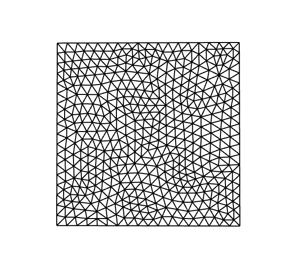
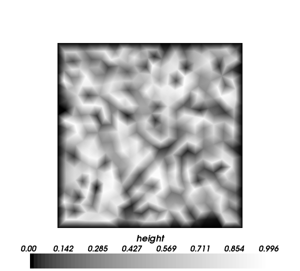
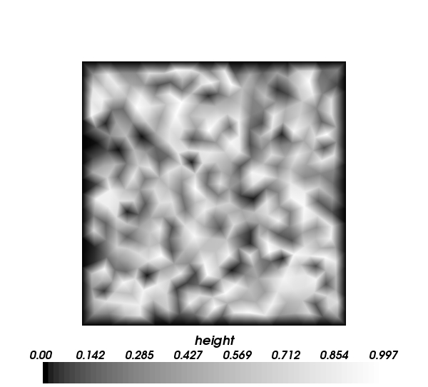
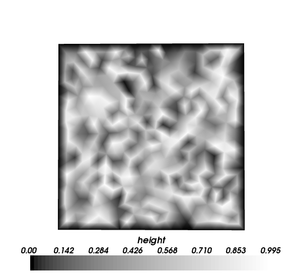
Fig. 1: Figure showing random $\eta^{\delta}$ fields used to verify the optimal balance property described in Theorem 12. Randomly generated $\eta^{\delta}$ and ${\boldsymbol{u}}^{\delta}$ fields (constrained to satisfy the balance conditions of the theorem) were used as initial conditions for a numerical integration with the implicit-midpoint rule in time applied to equations (11-12). The difference between the initial and final $\eta^{\delta}$ fields was observed to be numerically zero for all random realisations that were tested. Note that the steady state does not depend on the smoothness of the solution or on the mesh structure.

3.2 Inf-sup condition: pressure modes

We next prove that the discretisation given by equations (11-12) using a finite element pair satisfying our two conditions does not have any spurious pressure modes. These are modes which converge (in the limit as the mesh edge-lengths go to zero) to steady solutions with zero velocity even though the free surface displacement $\eta^{\delta}$ is not flat. These modes are catastrophic for discretisations of the nonlinear equations since they can grow to dominate the solution when coupled to the physical modes. These modes are not present if it is possible to bound the gradient of non-constant functions in $H$ from below as the edge-lengths go to zero. This bound is expressed in the following inf-sup condition:

Definition 15 (Inf-sup condition).

The inf-sup condition for a finite element pair $(H,V)$ requires that

$$\sup_{{\boldsymbol{w}}^{\delta}\in V}\frac{\int_{\Omega}{\boldsymbol{w}}^{\delta}\cdot\nabla\phi^{\delta}\operatorname{d}{V}}{\sqrt{\int_{\Omega}|{\boldsymbol{w}}^{\delta}|^{2}\operatorname{d}{V}}}\geq\beta\sqrt{\int_{\Omega}(\phi^{\delta})^{2}\operatorname{d}{V}},\quad\forall\phi^{\delta}\in H,$$ (18)

where $\beta$ is independent of the edge lengths in the mesh $\mathcal{M}$.

Theorem 16 (Inf-sup theorem).

Let $(H,V)$ be a finite element pair which satisfies condition 1 in definition 5. Then $(H,V)$ satisfies the inf-sup condition in definition 15.

Proof.

The supremum in equation (18) is bounded from below by any particular choice of test function ${\boldsymbol{w}}^{\delta}$. By condition 1 $\nabla\phi^{\delta}\in V$ and so we may choose ${\boldsymbol{w}}^{\delta}=\nabla\phi^{\delta}$. Substitution then gives

$$\sup_{{\boldsymbol{w}}^{\delta}\in V}\frac{\int_{\Omega}{\boldsymbol{w}}^{\delta}\cdot\nabla\phi^{\delta}\operatorname{d}{V}}{\sqrt{\int_{\Omega}|{\boldsymbol{w}}^{\delta}|^{2}\operatorname{d}{V}}} \geq \frac{\int_{\Omega}\nabla\phi^{\delta}\cdot\nabla\phi^{\delta}\operatorname{d}{V}}{\sqrt{\int_{\Omega}|\nabla\phi^{\delta}|^{2}\operatorname{d}{V}}}$$

$$= \sqrt{\int_{\Omega}|\nabla\phi^{\delta}|^{2}\operatorname{d}{V}}$$

$$= \sqrt{\frac{\int_{\Omega}|\nabla{\phi^{\delta}}|^{2}\operatorname{d}{V}}{\int_{\Omega}{\phi^{\delta}}^{2}\operatorname{d}{V}}}\sqrt{\int_{\Omega}{\phi^{\delta}}^{2}\operatorname{d}{V}},$$

$$\geq \sqrt{\lambda_{\min}}\sqrt{\int_{\Omega}{\phi^{\delta}}^{2}\operatorname{d}{V}},$$

where $\lambda_{\min}$ is the minimum non-zero eigenvalue of (minus) the Laplacian on $\Omega$, having made use of the Rayleigh quotient

$$\lambda_{\min}=\min_{\phi^{\delta}\neq 0}\frac{\int_{\Omega}|\nabla\phi^{\delta}|^{2}\operatorname{d}{V}}{\int_{\Omega}{\phi^{\delta}}^{2}\operatorname{d}{V}}.$$

∎

We note that the family of finite element pairs considered in this paper corresponds to one particular option for discrete differential forms satisfying a discrete de Rham complex condition described in [2]. In fact, condition 1 of Definition 5 corresponds to all of the options described in that paper.

A consequence of the inf-sup theorem, as discussed in [3, 1], is that the solutions of the wave equation converge at the optimal rate described by the theory of numerical interpolation, as described in the following corollary:

Corollary 17.

Given an interval $[0,T]$, there exists a constant $C(T)$ such that

$$\|{\boldsymbol{u}}(\cdot,T)-{\boldsymbol{u}}^{\delta}(\cdot,T)\|_{L_{2}}+\|\eta(\cdot,T)-\eta^{\delta}(\cdot,T)\|_{L_{2}}\leq C(T)h^{k+1}$$

where $({\boldsymbol{u}},\eta)$ is the solution of equations (7-8) with initial conditions $({\boldsymbol{u}}_{0},\eta_{0})$, $({\boldsymbol{u}}^{\delta},\eta^{\delta})$ is the solution of equations (11-12) with initial conditions $({\boldsymbol{u}}^{\delta}_{0},\eta^{\delta}_{0})$ which satisfy the interpolation condition

$$\|{\boldsymbol{u}}^{\delta}_{0}-{\boldsymbol{u}}_{0}\|_{L_{2}}+\|\eta^{\delta}_{0}-\eta_{0}\|_{L_{2}}\leq ch^{k+1}$$

and where $k$ is the minimum of the orders of the elementwise polynomials used to construct ${\boldsymbol{u}}^{\delta}$ and $\eta^{\delta}$.

Proof.

The proof follows using standard mixed finite element techniques, namely obtaining a bound on the $L_{2}$-norm of the solution variables ${\boldsymbol{u}}^{\delta}$ and $\eta^{\delta}$ which requires the inf-sup condition. See [11], [3] or [1], for example. ∎

For the $\textrm{P1}_{\textrm{DG}}$-P2 element pair, this convergence property (in this case 2nd-order convergence since $k=1$) was confirmed from numerical experiments for the 2-dimensional wave equation in [5], and for the rotating linear shallow-water equations on an $f$-plane in [4].

4 Three dimensional incompressible flow

In this section we briefly discuss the extension of these properties to the equations of three dimensional rotating stratified nonhydrostatic incompressible flow (Boussinesq equations) which, together with their hydrostatic counterparts, are used in ocean modelling.

4.1 Model equations and geostrophic states

The full equations of motion are:

$${\boldsymbol{u}}_{t}+({\boldsymbol{u}}\cdot\nabla){\boldsymbol{u}}+f{\boldsymbol{k}}\times{\boldsymbol{u}} = -\frac{1}{\rho_{0}}\nabla p+{\boldsymbol{k}}b,$$ (19)

$$\nabla\cdot{\boldsymbol{u}} = 0,$$ (20)

$$T_{t}+{\boldsymbol{u}}\cdot\nabla T = 0,$$ (21)

where ${\boldsymbol{u}}$ is the three-dimensional velocity field, $f$ is the Coriolis parameter, ${\boldsymbol{k}}$ is the unit upward vector, $p$ is the pressure, $b$ is the buoyancy and $T$ is the temperature (salinity would also be included in a full ocean model but does not add anything to this discussion). The system is closed by specifying an equation of state in which the buoyancy $b$ is defined as a function of $T$ and $p$. Here we have made the traditional approximation which restricts the rotation vector to the vertical axis, and the $f$-plane approximation for which $f$ is a constant.

In three dimensions there are two geophysical balances which are present in slowly-varying large-scale flows which arise when the acceleration terms are small compared to the Coriolis and buoyancy. In the vertical direction we obtain the hydrostatic balance

$$-\frac{1}{\rho_{0}}p_{z}+b=0,$$ (22)

which can be imposed as a constraint in a hydrostatic model, allowing the pressure to be computed explicitly from the buoyancy by vertical integration. In the horizontal direction we again obtain the geostrophic balance

$$u=-\frac{1}{\rho_{0}f}p_{y},\quad v=\frac{1}{\rho_{0}f}p_{x}.$$ (23)

It is simple to check again that $\nabla\cdot{\boldsymbol{u}}=0$ for these balanced states. In the case of incompressible flow, this means that the balanced states are solutions of the equations given above.

One can again take a numerical discretisation of equations (19-21), construct the discrete balanced solutions and check if the discrete form of equation 20 is satisfied exactly. If there is some residual, then this means that it is not possible for exactly-balanced states to exist in the numerical discretisation, which can lead to to the generation of spurious internal inertia-gravity waves. For example, if a pressure-projection method is used for timestepping (as is typical for non-hydrostatic models) then the time-integrator has two stages: the first stage takes a momentum step using the pressure from the previous timestep, then the solution is projected back to satisfy the discrete form of equation 20. If the balanced states do not satisfy this equation, then each projection will generate further spurious unbalanced motion.

In this section we shall briefly describe an extension of our family of finite-element pairs to the three-dimensional case, and describe the extension of our optimal balance results. Since we are still concerned with wave propagation we linearise equations (19-21) about the state

$${\boldsymbol{u}}=0,\quad p_{z}=\rho_{0}b,\quad T=\bar{T}({\boldsymbol{z}}),$$

to obtain

$${\boldsymbol{u}}_{t}+f{\boldsymbol{k}}\times{\boldsymbol{u}} = -\frac{1}{\rho_{0}}\nabla p^{\prime}+{\boldsymbol{k}}\gamma T^{\prime},$$ (24)

$$\nabla\cdot{\boldsymbol{u}} = 0,$$ (25)

$$T^{\prime}_{t}+u_{3}\bar{T}_{z} = 0,$$ (26)

where $\gamma$ is a suitable positive constant. We shall drop the primes for the rest of the section. For these equations, steady balanced states given by

$$u_{3}=0,\quad p_{z}=\rho_{0}\gamma T,\quad u=-\frac{1}{\rho_{0}f}p_{y},\quad v=\frac{1}{\rho_{0}f}p_{x},$$

satisfy $\nabla\cdot{\boldsymbol{u}}=0$ and hence are admissible solutions of the equations.

4.2 Finite element formulation

Defining a Galerkin finite element method for these equations requires us to define a finite element space $\Theta$ for the temperature variable $T^{\delta}$. The choice of this space is not very important for the discussion of geostrophically-balanced states, so it will not be developed much here, except to note that it is important to ensure that there are sufficiently many states which satisfy a discrete hydrostatic balance, otherwise the representation of hydrostatic balance will be poor, leading to spurious non-hydrostatic motion. The velocity space $V$ and the pressure space $H$ are defined by the three dimensional extensions of definitions 1-3.

We now define the Galerkin finite element method for equations (24-26) as follows:

Definition 18 (Galerkin finite element method for 3D wave propagation).

${\boldsymbol{u}}^{\delta}({\boldsymbol{x}},t)$, $p^{\delta}({\boldsymbol{x}},t)$, $T^{\delta}({\boldsymbol{x}},t)$ are the semi-discrete solutions of the Galerkin finite element discretisation of (24-26) if

$${\boldsymbol{u}}^{\delta}(\cdot,t)\in V,\quad p^{\delta}(\cdot,t)\in H,\quad T^{\delta}(\cdot,t)\in\Theta,\qquad\forall t\in[0,T],$$

and

$$\frac{\operatorname{d}}{\operatorname{d}t}\int_{\Omega}{\boldsymbol{w}}^{\delta}\cdot{\boldsymbol{u}}^{\delta}\operatorname{d}{V}+f\int_{\Omega}{\boldsymbol{w}}^{\delta}\cdot{\boldsymbol{k}}\times{\boldsymbol{u}}^{\delta}\operatorname{d}{V} = -\frac{1}{\rho_{0}}\int_{\Omega}{\boldsymbol{w}}^{\delta}\cdot\nabla p^{\delta}\operatorname{d}{V}+\gamma{\boldsymbol{k}}\cdot\int_{\Omega}{\boldsymbol{w}}^{\delta}T^{\delta}\operatorname{d}{V},$$ (27)

$$-\int_{\Omega}\nabla\phi^{\delta}\cdot{\boldsymbol{u}}^{\delta}\operatorname{d}{V} = 0,$$ (28)

$$\frac{\operatorname{d}}{\operatorname{d}t}\int_{\Omega}\theta^{\delta}T^{\delta}\operatorname{d}{V}+{\boldsymbol{k}}\cdot\int_{\Omega}\theta^{\delta}{\boldsymbol{u}}^{\delta}\bar{T}^{\delta}_{z}\operatorname{d}{V} = 0,$$ (29)

for all test functions ${\boldsymbol{w}}^{\delta}\in V$, $\phi^{\delta}\in H$, $\theta^{\delta}\in\Theta$.

We again require our element pair $(H,V)$ to satisfy the conditions in Definition 5, extended to three dimensions (with the $\perp$ operator replaced by the ${\boldsymbol{k}}\times$ operator). We next define the discrete geophysical balances using this discretisation.

Definition 19 (Discrete hydrostatic and geostrophic balance).

The solution variables ${\boldsymbol{u}}^{\delta}$, $p^{\delta}$ and $T^{\delta}$ satisfy the hydrostatic and geostrophic balances if

$$f\int_{\Omega}{\boldsymbol{w}}^{\delta}\cdot{\boldsymbol{k}}\times{\boldsymbol{u}}^{\delta}\operatorname{d}{V}=-\frac{1}{\rho_{0}}\int_{\Omega}{\boldsymbol{w}}^{\delta}\cdot\nabla p^{\delta}\operatorname{d}{V}+\gamma{\boldsymbol{k}}\cdot\int_{\Omega}{\boldsymbol{w}}^{\delta}T^{\delta}\operatorname{d}{V}.$$ (30)

The vertical component specifies hydrostatic balance and the horizontal component specifies geostrophic balance.

This definition allows us to state the optimal balance theorem for three-dimensional incompressible flow, which we give in the next subsection.

4.3 Optimal balance properties, inf-sup theorem and optimal pressure matrix property

Theorem 20 (Optimal balance for three-dimensional incompressible flow).

Let ${\boldsymbol{u}}^{\delta}\in V$, $p^{\delta}\in H$ and $T^{\delta}\in\Theta$ be chosen so that equation (30) is satisfied, with zero vertical velocity $u^{\delta}_{3}=0$ and the pressure $p^{\delta}$ satisfying the pointwise condition

$${\boldsymbol{\tau}}_{H}\cdot\nabla p^{\delta}=0,\quad\forall{\boldsymbol{x}}\in\partial\Omega,$$

where $\tau_{H}$ is the horizontal tangent vector to $\partial\Omega$ so that the boundary is a streamline for the balanced flow (consistent with the boundary condition for ${\boldsymbol{u}}^{\delta})$. Then $({\boldsymbol{u}}^{\delta},p^{\delta},T^{\delta})$ is a steady state solution of equations (27-29).

Proof.

It is simple to check that ${\boldsymbol{T}}^{\delta}_{t}=0$, ${\boldsymbol{u}}^{\delta}_{t}=0$ by inserting the solutions into the equations and noting that all of the terms vanish, and it remains to check that equation 28 is satisfied. The proof proceeds exactly as the proof of Theorem 12, by first noting that the two conditions in Definition 5 imply that

$${\boldsymbol{u}}^{\delta}=(-\psi^{\delta}_{y},\psi^{\delta}_{x}),\quad\psi^{\delta}=\frac{1}{f\rho_{0}}p^{\delta}$$

pointwise, which we then insert into equation 28 to obtain

$$-\int_{\Omega}\nabla\phi^{\delta}\cdot{\boldsymbol{u}}^{\delta}\operatorname{d}{V}=\int_{\Omega}\phi^{\delta}_{x}\psi^{\delta}_{y}-\phi^{\delta}_{y}\psi^{\delta}_{x}\operatorname{d}{V}=0,$$

using a similar argument to the previous proof. ∎

This means that balanced states are exactly steady and do not generate any spurious internal waves. Note that this theorem is again completely independent of the mesh structure and so the finite element pairs in this family are ideal for representing balanced flows on unstructured meshes such as those proposed in [18].

As for the 2D case, it is necessary for the finite element spaces to satisfy an inf-sup condition, so that solutions of the linearised equations converge at the optimal rate defined by approximation theory. In the case of incompressible flow, one also forms a pressure Poisson equation by composing the discrete divergence and gradient operators, and if the inf-sup condition is not satisfied then there are very small spurious eigenvalues in the matrix which make iterative solvers very slow (see [10], for example). Our family of finite element pairs satisfy the inf-sup condition in three dimensions which can be shown by simple extension of the proof of Theorem 16. For incompressible flow, we shall use the same techniques to prove further properties of the discrete Poisson matrix.

For the continuous equations, the Poisson equation is formed by taking the divergence of equation (24) and applying equation (25) to obtain

$$\nabla^{2}p=\nabla\cdot{\boldsymbol{r}}=\nabla\cdot(\rho_{0}{\boldsymbol{k}}\gamma T-\rho_{0}f{\boldsymbol{k}}\times{\boldsymbol{u}}),$$ (31)

which specifies an equation for $p$ given $T$ and ${\boldsymbol{u}}$. This equation must be solved at each timestep to calculate the pressure field. When the Galerkin finite element method is applied, this specifies a coupled system of equations for ${\boldsymbol{p}}$ given by

$$\int_{\Omega}{\boldsymbol{w}}^{\delta}\cdot{\boldsymbol{r}}^{\delta}\operatorname{d}{V} = -\rho_{0}f\int_{\Omega}{\boldsymbol{w}}^{\delta}\cdot{\boldsymbol{k}}\times{\boldsymbol{u}}^{\delta}\operatorname{d}{V}+\rho_{0}\gamma{\boldsymbol{k}}\cdot\int_{\Omega}{\boldsymbol{w}}^{\delta}T^{\delta}\operatorname{d}{V},$$ (32)

$$\int_{\Omega}{\boldsymbol{w}}^{\delta}\cdot{\boldsymbol{q}}^{\delta}\operatorname{d}{V} = \int_{\Omega}{\boldsymbol{w}}^{\delta}\cdot\nabla{\boldsymbol{p}}^{\delta}\operatorname{d}{V},$$ (33)

$$\int_{\Omega}\nabla\phi^{\delta}\cdot{\boldsymbol{q}}^{\delta}\operatorname{d}{V} = -\int_{\Omega}\nabla\phi^{\delta}\cdot{\boldsymbol{r}}^{\delta}\operatorname{d}{V},$$ (34)

for $p^{\delta}\in H$, ${\boldsymbol{q}}^{\delta},{\boldsymbol{r}}^{\delta}\in V$ and for all test functions $\phi^{\delta}\in H$ and ${\boldsymbol{w}}^{\delta}\in V$. In practise, the variables ${\boldsymbol{q}}^{\delta}$ and ${\boldsymbol{r}}^{\delta}$ are eliminated to obtain an equation for $p^{\delta}$. This then ensures that equation (28) is satisfied at each instance in time (or each timestep, having discretised the equations in time). This system gives rise to a matrix equation for the basis function coefficients which, in general can have a larger sparsity pattern since it involve the product of several matrices (see [10], for example). In the following theorem, we show that this sparsity pattern is reduced when condition 1 of Definition 5 is satisfied, which is a further useful property of the family of finite element pairs discussed in this paper.

Theorem 21 (Optimal sparsity of pressure matrix).

Let $p^{\delta}$, ${\boldsymbol{q}}^{\delta}$, ${\boldsymbol{r}}^{\delta}$ be the solutions of equations (32-33). Then

$$\int_{\Omega}\nabla\phi^{\delta}\cdot\nabla p^{\delta}\operatorname{d}{V}=-\int_{\Omega}\nabla\phi^{\delta}\cdot{\boldsymbol{r}}^{\delta}\operatorname{d}{V},$$ (35)

for all test functions $\phi^{\delta}\in H$, which is the usual Galerkin discretisation for equation (31).

Proof.

We again make use of lemma 10 which states that

$${\boldsymbol{q}}^{\delta}=\nabla p^{\delta}$$

at each point. Substitution into equation (34) gives the result. ∎

Since the usual Galerkin discretisation of equation (31) results in a single equation that does not require the elimination of variables, this results in a much sparser stencil for the matrix equation for the basis function coefficients of $p^{\delta}$.

5 Summary and outlook

In this paper we defined a large family of finite element discretisations for the rotating shallow-water equations and the three dimensional equations of rotating stratified incompressible flow. When applied to the linear rotating shallow water equations, these discretisations were shown satisfy the optimal property that geostrophically-balanced states are completely steady, which mirrors a property of the solutions of the continuous equations. It was also shown that the discretisations in the family satisfy an inf-sup condition which prohibits the existence of spurious pressure modes. This makes the discretisations in the family strong candidates for use in NWP and ocean modelling in cases where triangular elements are required, e.g. to allow the use of geodesic grids. Furthermore, the proofs are independent of the mesh structure which means that the family of discretisations produce stable results in the presence of adaptive mesh refinement. We then discussed the extension of the family to three-dimensional incompressible flow, required for ocean modelling, and showed that the discretisations in the family result in exactly steady balanced states on completely arbitrary unstructured meshes in three dimensions. In addition, the properties of the family were used to show that the matrix obtained from the discretised pressure Poisson equation has an optimally sparse stencil.

In future work, we will develop and test discretisations of the fully-nonlinear equations using choices from our family of finite element spaces, particularly from the $\textrm{Pn}_{\textrm{DG}}$-P(n+1) sub-family applied to the rotating shallow-water equations and the three dimensional incompressible equations. Elements of that sub-family have discontinuous velocity, which allows a discontinuous Galerkin treatment of the advection terms in the momentum equation. We also plan to compute numerical dispersion relations for these discretisations when applied to the geodesic grid, in order to make comparisons with other element pairs and finite difference methods on this grid. The $\textrm{P1}_{\textrm{DG}}$-P2 element is currently being implemented in the Imperial College Ocean Model, and will be developed into a $p$-adaptive scheme in which different order polynomials are used in different elements.

References

- [1] Douglas N. Arnold, Richard S. Falk, and Ragnar Winther. Differential complexes and stability of finite element methods. I. the de Rham complex. In IMA Volumes in Mathematics and its Applications, volume 142, pages 47–68. Springer, 2006.
- [2] Douglas N. Arnold, Richard S. Falk, and Ragnar Winther. Finite element exterior calculus, homological techniques, and applications. Acta Numerica, 15:1–155, 2006.
- [3] F. Auricchio, F. Brezzi, and C. Lovadina. Mixed finite element methods. In Encyclopedia of Computational Mechanics, volume 1, chapter 9. Wiley, 2004.
- [4] C. J. Cotter, D. A. Ham, and C. C. Pain. A mixed discontinuous/continuous finite element pair for shallow-water ocean modelling. Ocean Modelling, 26:86–90, 2009.
- [5] C. J. Cotter, D. A. Ham, C. C. Pain, and S. Reich. LBB stability of a mixed finite element pair for fluid flow simulations. J. Comp. Phys., 228(3):336–348, 2009.
- [6] C. J. Cotter and S. Reich. Semigeostrophic particle motion and exponentially accurate normal forms. Multiscale Model Sim., 5:476–496, 2006.
- [7] T. Davies, M. J. P. Cullen, A. J. Malcolm, M. H. Mawson, A. Staniforth, A. A. White, and N. Wood. A new dynamical core for the Met Office’s global and regional modelling of the atmosphere. Q. J. Roy. Met. Soc, 131(608):1759–1782, 2005.
- [8] L. C. Evans. Partial Differential Equations. Grad. Stud. Math. Amer. Math. Soc., 1998.
- [9] R. Ford, M.E. McIntyre, and W.A. Norton. Balance and the slow quasimanifold: Some explicit results. J. Atmos. Sci., 57:1236–1254, 2000.
- [10] P. M. Gresho and R. L. Sani. Incompressible Flow and the Finite Element Method, Volume 2, Isothermal Laminar Flow. Wiley, 2000.
- [11] Patrick Joly. Topics in Computational Wave Propagation: Direct and Inverse Problems, chapter 6. Springer, 2003.
- [12] D.Y. Le Roux, A. Sène, V. Rostand, and E. Hanert. On some spurious mode issues in shallow-water models using a linear algebra approach. Ocean Modelling, pages 83–94, 2005.
- [13] D.Y. Le Roux, A. Staniforth, and C. A. Lin. Finite elements for shallow-water equation ocean models. Monthly Weather Review, 126(7):1931–1951, 1998.
- [14] D. Majewski, D. Liermann, P. Prohl, B. Ritter, M. Buchhold, T. Hanisch, G. Paul, W. Wergen, , and J. Baumgardner. The operational global icosahedral–hexagonal gridpoint model GME: Description and high-resolution tests. Mon. Wea. Rev., 130:319–338, 2002.
- [15] M. E. McIntyre and W.A. Norton. Potential vorticity inversion on a hemisphere. J. Atmos. Sci., 57:1214–1235, 2000.
- [16] A. R. Mohebalhojeh and D.G. Dritschel. Hierarchies of balance conditions for the f-plane shallow-water equations. J. Atmos. Sci., 58:2411–2426, 2001.
- [17] E. I. Olfasdottir, A. B. Olde Daalhuis A. B., and J. Vanneste. Inertia-gravity-wave generation by a sheared vortex. J. Fluid Mech., 569:169–189, 2008.
- [18] C.C. Pain, M.D. Piggott, A.J.H. Goddard, F. Fang, G.J. Gorman, D.P. Marshall, M.D. Eaton, P.W. Power, and C.R.E. de Oliveira. Three-dimensional unstructured mesh ocean modelling. Ocean Modelling, 10:5–33, 2005.
- [19] Raviart and Thomas. A mixed finite element method for 2nd order elliptic problems. In Mathematical Aspects of the Finite Element Method, Lecture Notes in Mathematics. Springer, Berlin, 1977.
- [20] T. D. Ringler, R.P. Heikes, , and D.A. Randall. Modeling the atmospheric general circulation using a spherical geodesic grid: A new class of dynamical cores. Mon. Wea. Rev., 128:2471–2490, 2000.
- [21] R. L. Salmon. Lectures on Geophysical Fluid Dynamics. OUP, 1998.
- [22] M. Satoh, T. Matsuno, H. Tomita, H. Miura, T. Nasuno, and S. Iga. Nonhydrostatic icosahedral atmospheric model (NICAM) for global cloud resolving simulations. J. Comp. Phys., 227(7):3486–3514, 2008.
- [23] J. Thuburn. Numerical wave propagation on the hexagonal C-grid. J. Comp. Phys., 227(11):5836–5858, 2008.
- [24] G. Umgiesser, D. M. Canu, A. Cucco, and C. Solidoro. A finite element model for the Venice Lagoon. Development, set up, calibration and validation. Journal of Marine Systems, 51(1-4):123–145, 2004.
- [25] R.A. Walters and V. Casulli. A robust, finite element model for hydrostatic surface water flows. Communications in Numerical Methods in Engineering, 14:931–940, 1998.